Introduction
The COVID-19 pandemic first emerged in Wuhan, China as a novel zoonotic coronavirus in December 2019 (Diamond and Wood, 2020). The virus quickly spread westward and was first detected in Texas on February 7th, 2020. COVID-19 has resulted in over 4.3 million confirmed cases and over 290,000 deaths across the globe by July 2020 (Nicola, et al., 2020, Stein Zweers 2022). The spread of this highly contagious respiratory disease triggered a global shutdown of socio-economic activities. The contraction of the global economy corresponded with restricted travel patterns and reduced greenhouse gas emissions from human inputs.
Anthropogenic factors that contribute to atmospheric pollution are largely driven by heavy industrial economies (e.g., manufacturing and oil production) as well as domestic sources (e.g., vehicle exhaust). Typical compounds such as nitrogen oxides, sulphides and aerosols are all major components of air pollution (Weinstock, 1969 and Junge, 1974). These fine particles known as aerosols are classed as PM 2.5 with aerodynamic diameters of 2.5 micrometers or less (Burnett, et al., 2018). PM 2.5 poses a public health risk, especially to respiratory sensitive groups, and is responsible for roughly 10 million deaths annually (Burnett, et al., 2018). Aerosols influence climatic conditions by absorbing and scattering sunlight. High aerosol concentrations in the atmosphere are responsible for radiative forcing, causing a positive feedback in the climate system (Diamond and Wood, 2020). Particles suspended in the atmosphere increase with pollutants expelled from high exhaust points such as vehicles and heavy industrial zones. Intuitively, the global lockdown conditions introduce a novel case in the reduction of atmospheric compounds as a result of reduced human activity. Changes in emission rates are recorded across the globe, with the strongest declines observed in the United States, South Korea, Europe and China (Bauwens et al., 2020). This paper discusses the changes in atmospheric gases and aerosols immediately before and after lockdown conditions in the major cities in Texas (San Antonio, Houston, Dallas and Austin) alongside Wuhan, China.
Data and Methods
Google Earth Engine (GEE) is an open source datahub useful for data compilation and analysis. Sentinel products as published by the European Space Agency (ESA), is one such dataset available for use through the GEE. Sentinel includes an atmospheric monitoring instrument aboard the satellite known as Sentinel-5P. This study utilizes the Sentinel-5P TROPOMI (Tropospheric Monitoring Instrument) to analyze the monthly mean trends in greenhouse gases and aerosols from July 2018 to July 2020. Sentinel 5P was launched by the ESA on October 13th 2017, to monitor air pollution. The instrument observes from nadir, with a nominal swath width of approximately 2,600 km (typical pixel size of 7 x 7 km2). The TROPOMI is a pushbroom imaging spectrometer with a wide field-of-view which allows daily coverage. The data provided are continuous high resolution spectral measurements in ultraviolet (UV), visible (VIS), near-infrared (NIR) and short-wave infrared (SWIR) bands. Measurements are taken on the day-side of the orbit at a mean solar time of 13:30 in near real time.
Sentinel-5P offers a host of products available for analysis, namely: UV aerosol index, sulphur dioxide, nitrogen dioxide, carbon monoxide, ozone, water vapor, cloud surface albedo and methane. The data retrieved through Google Earth Engine are Level-2 products which are geolocated total columns of ozone, sulphur dioxide, nitrogen dioxide, carbon monoxide, cloud and aerosol information. Google Earth Engine hosts Sentinel 5P source data that is filtered to remove pixels with QA values less than 80%, 75% and 50% for UVAI, Tropospheric nitrogen dioxide and all other datasets except for ozone and sulphur dioxide, respectively.
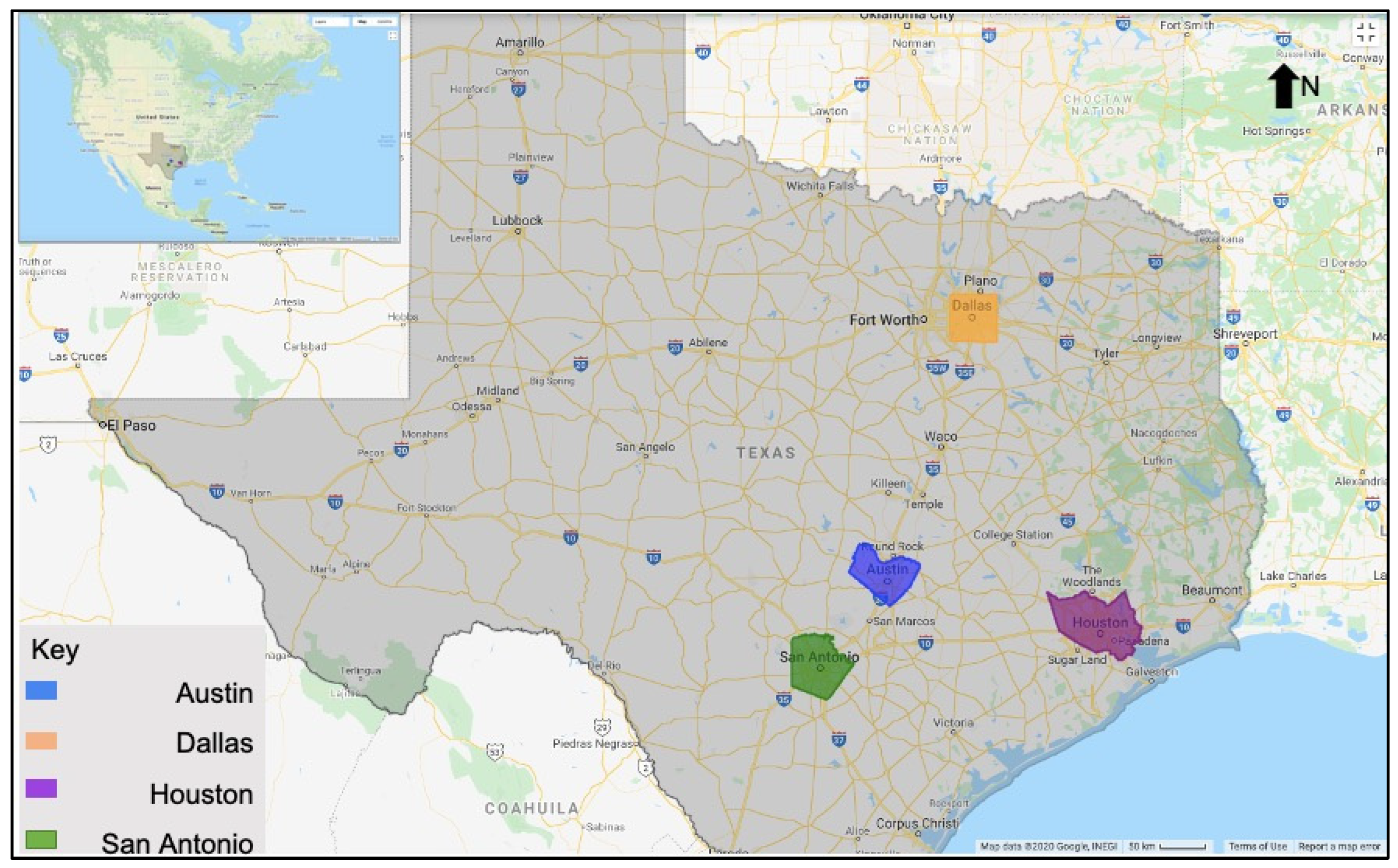
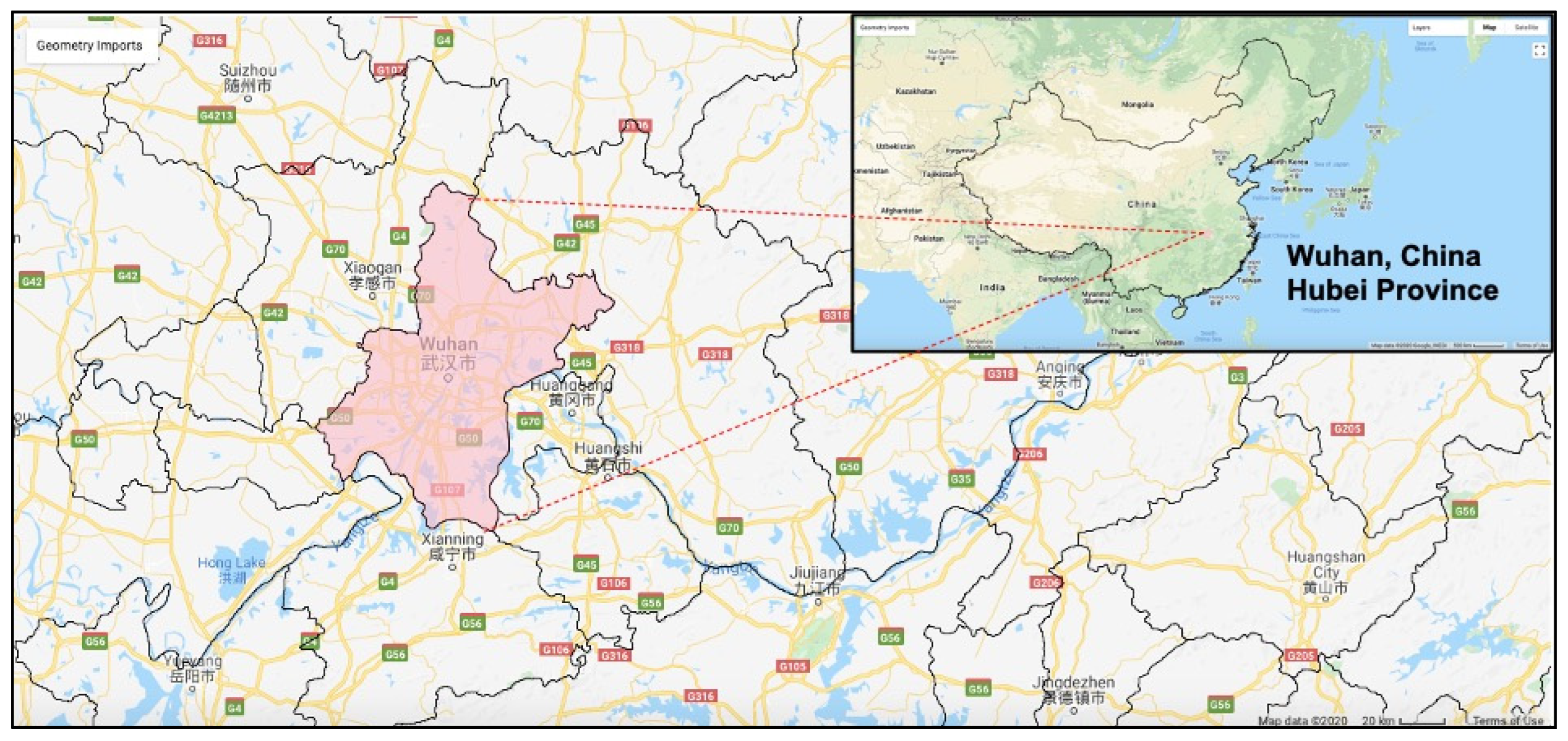
Google Earth Engine is used to retrieve and compile the monthly mean atmospheric column densities for select products over Wuhan, China and major Texan cities; Dallas, Houston, Austin and San Antonio. The regions of interest are shown in
Figure 1 and
Figure 2. To achieve this, the forenamed regions of interest are outlined using the US Topology Integrated Geographic Encoding and Referencing (TIGER) Federal Information Processing System (FIPS) spatial data for states. From this, the vertical column density of each compound is extracted for analysis. UVAI is one compound that is derived (Stein Zweers, 2022) and is calculated by equation 1 using the 354/388 wavelength pair.
where
are the calculated and measured reflectance of the atmospheric system, A
LER is the real surface albedo if there are no clouds or aerosols present. The data is then examined for missing data and are removed. The data is then compiled for the monthly mean of each compound for the respective region.
Results and Discussion
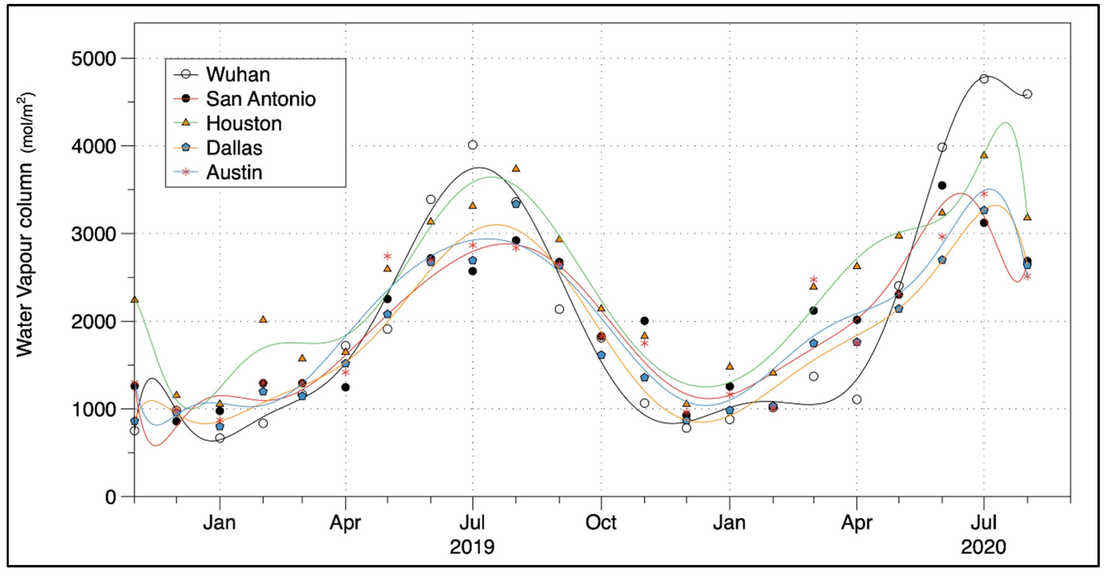
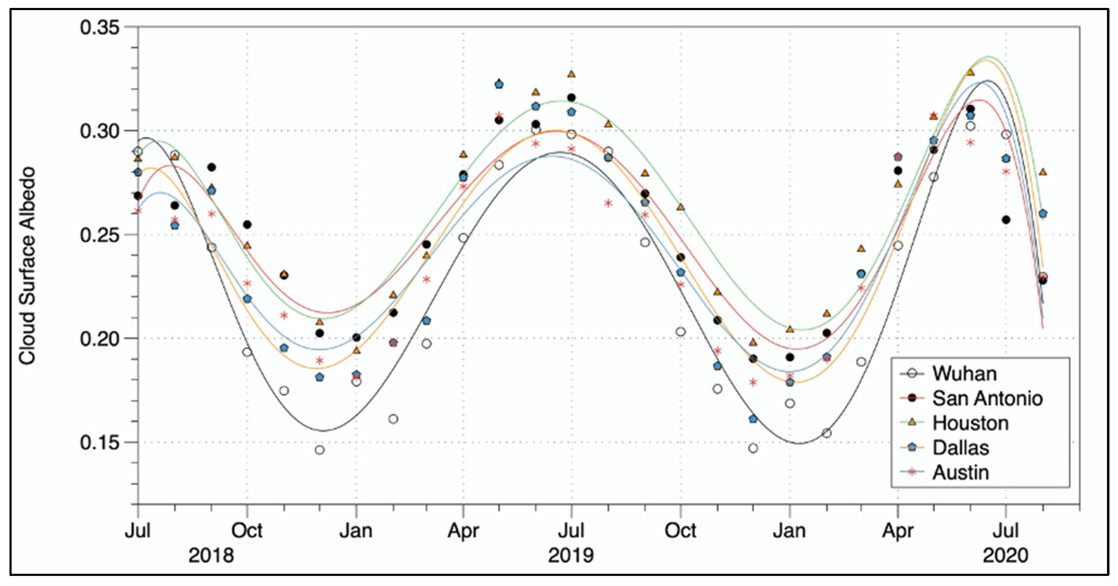
The relationship between aerosol prevalence, cloud condensate nuclei (water vapor content) and cloud surface albedo are displayed in this study through
Figure 3 and
Figure 4. Decreasing aerosol or PM2.5/10 in the atmosphere coincides with decreasing water vapor column and cloud surface albedo. The water vapor column however, shows more variance in its trend in comparison to the cloud albedo (optical thickness). During July, both the cloud albedo and water vapor column are at their peak each year suggesting more water storage in the atmosphere at the height of the Summer. The inverse is true for the Autumn and Winter months. Cloud albedo can indicate the atmosphere’s ability to promote chemical reactions between sunlight and greenhouse particles by their rate of absorption of solar energy. Still, this dynamic is spontaneous and difficult to assess their instantaneous relationships.
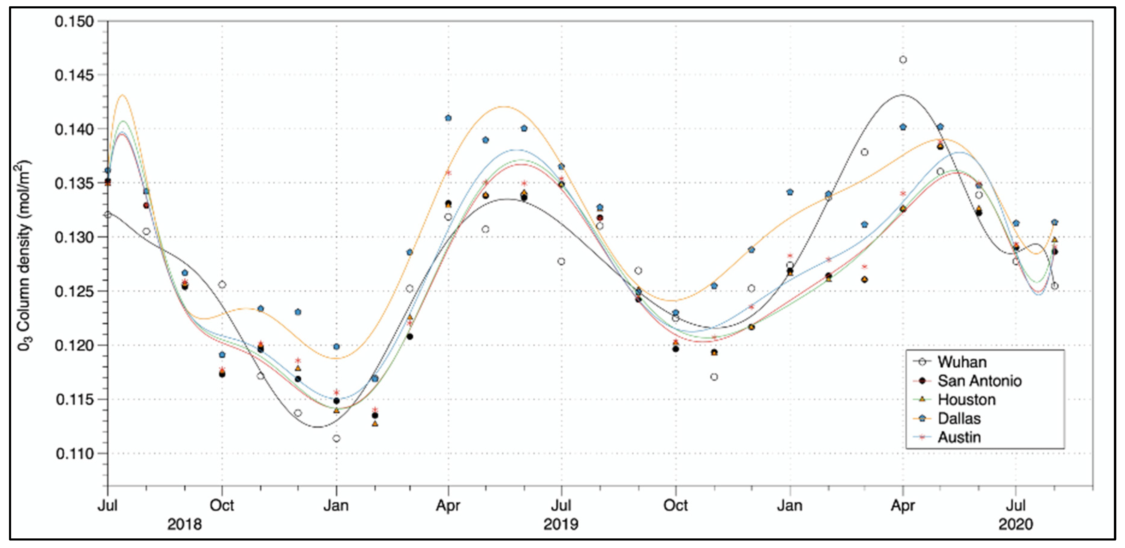
The resultant effect of chemical reactions between sunlight and volatiles is an increased ozone column density. Ozone total column density in
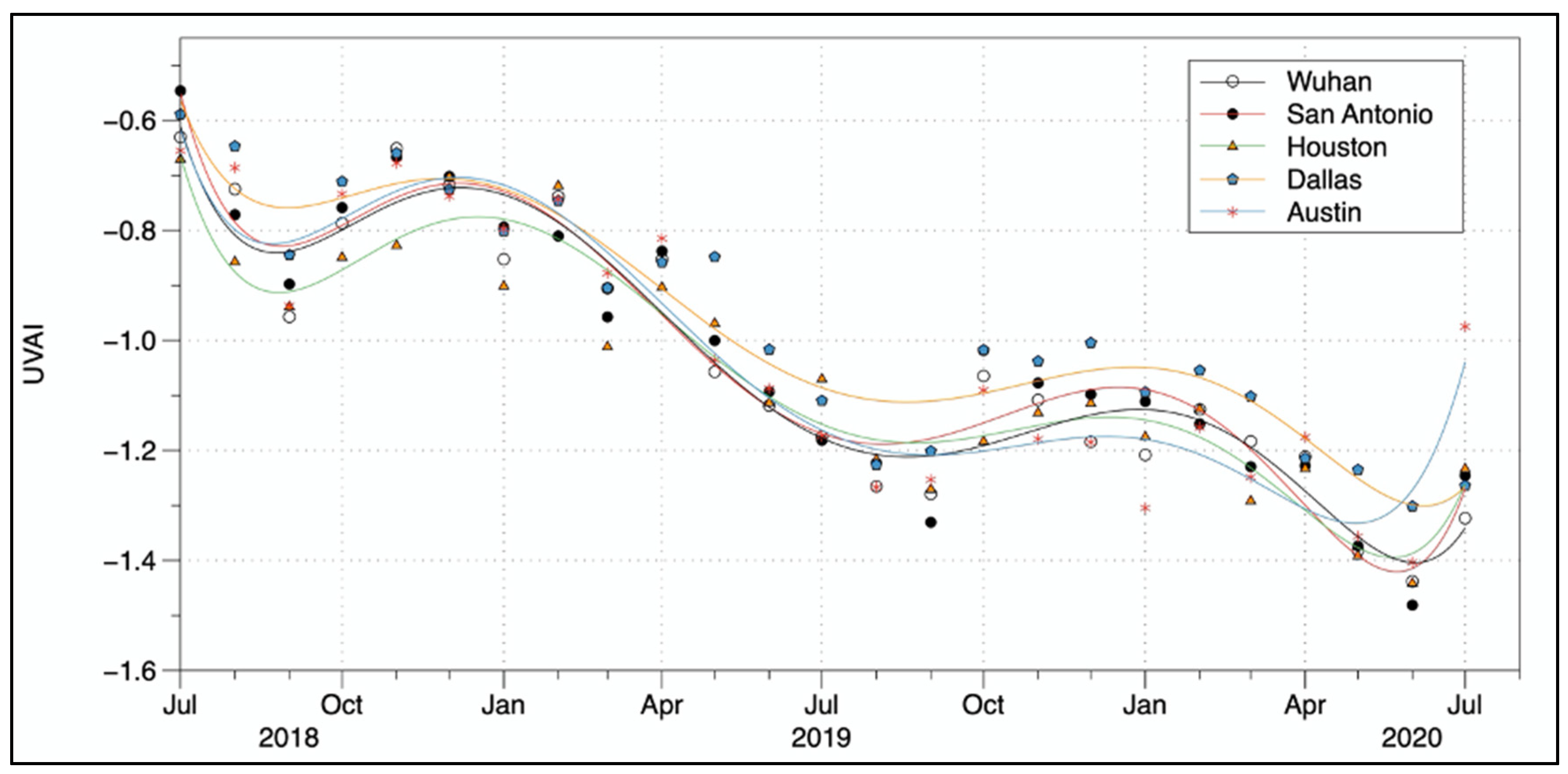
Figure 5 is highest over Wuhan as incident and reflected sunlight availability increases with increasing water vapor particles. During the lockdown periods previously described in both countries, the peak Ultraviolet Aerosol Index (UVAI) is lower than the previous year.
Figure 6 shows the time series of UVAI for the cities mentioned. The UVAI has decreased for all cities at the beginning of 2020 compared to the previous year. This is a function of reduced pollutants present in the air column. The cresting in January 2020 (
Figure 6) reflects typical background response such as pollen and naturally occurring dust.
This is in contrast with the peak in January 2019 which is reflective of background inputs and anthropogenic sources.
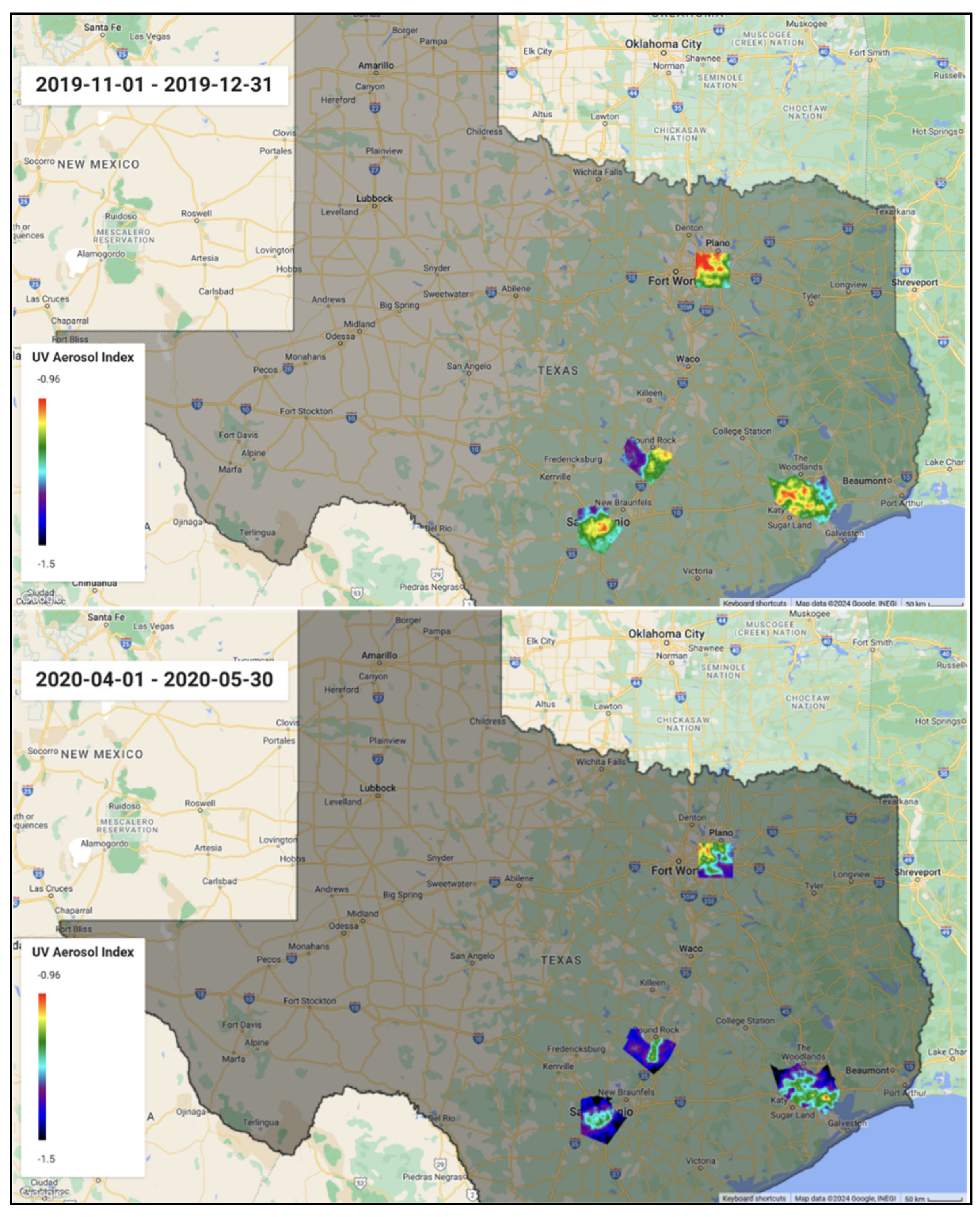
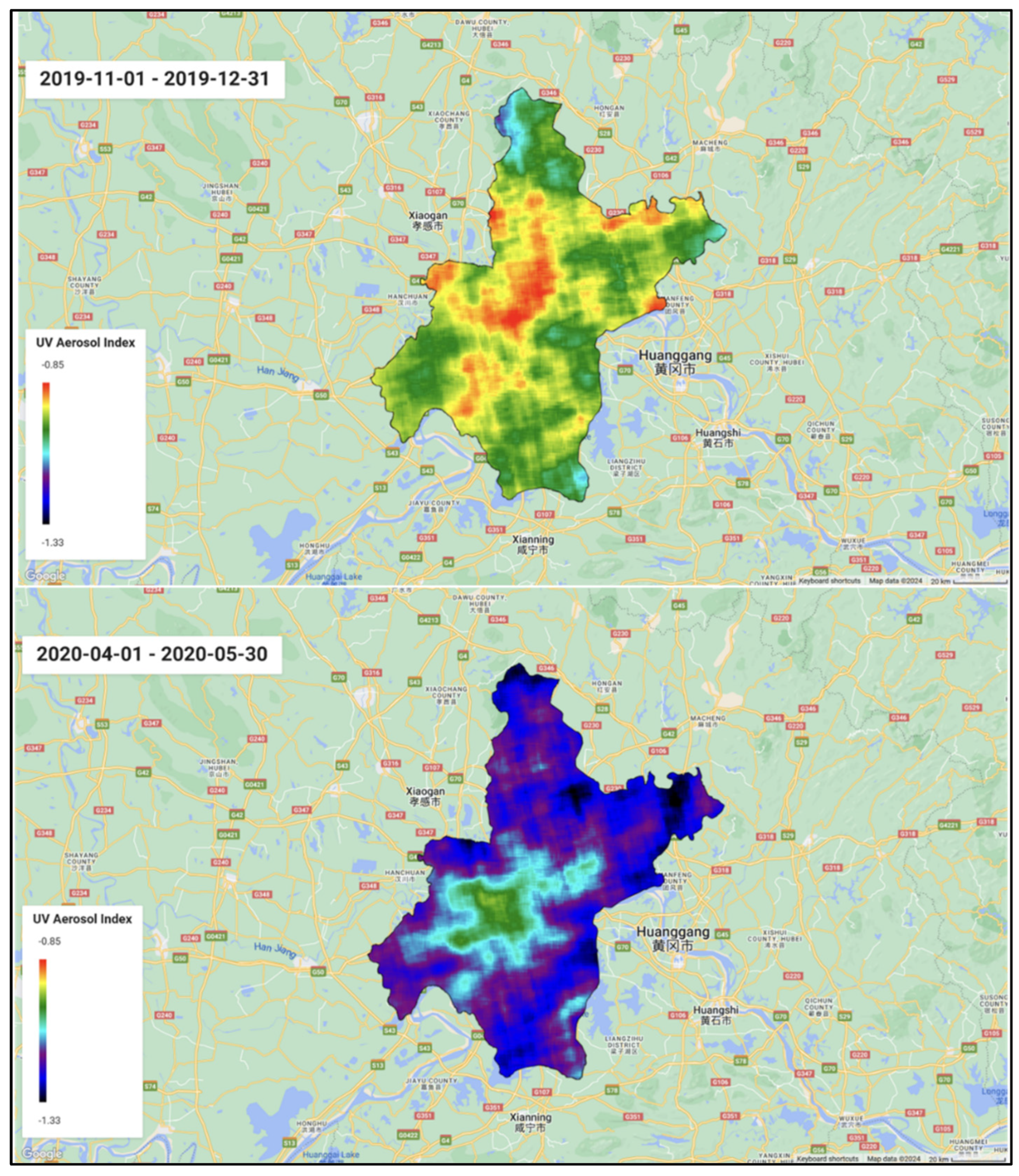
Figure 7 and
Figure 8 show the change in UVAI over Texas and Wuhan before and after the global shutdown with difference maps in all cases taken as the date before minus the date after. The change in UVAI ranges between 36.5 and 63.6% in Texas, with Dallas and Austin showing the smallest and largest reduction rates respectively. In China, Wuhan’s UVAI shows a reduction of 41.8%.
The figures show that there are specific UVAI hotspots that appear cooler after the global shutdown. However, the distribution of the higher and lower concentrations in space are similar. In the case of Texas, Houston and Dallas show higher UVAI concentrations when compared to Austin and San Antonio. Intuitively, these cities are larger with higher population densities and therefore higher emission rates. However, while Dallas maintains higher UVAI rates than other Texan cities after the shutdown conditions, San Antonio replaces Houston as the second highest emitter. This may speak to the varying shutdown constraints during lockdown imposed by each city. Foot-traffic information shows Houston had higher rates of compliance to shelter-in-place orders restrictions than San Antonio by roughly two percent (2%).
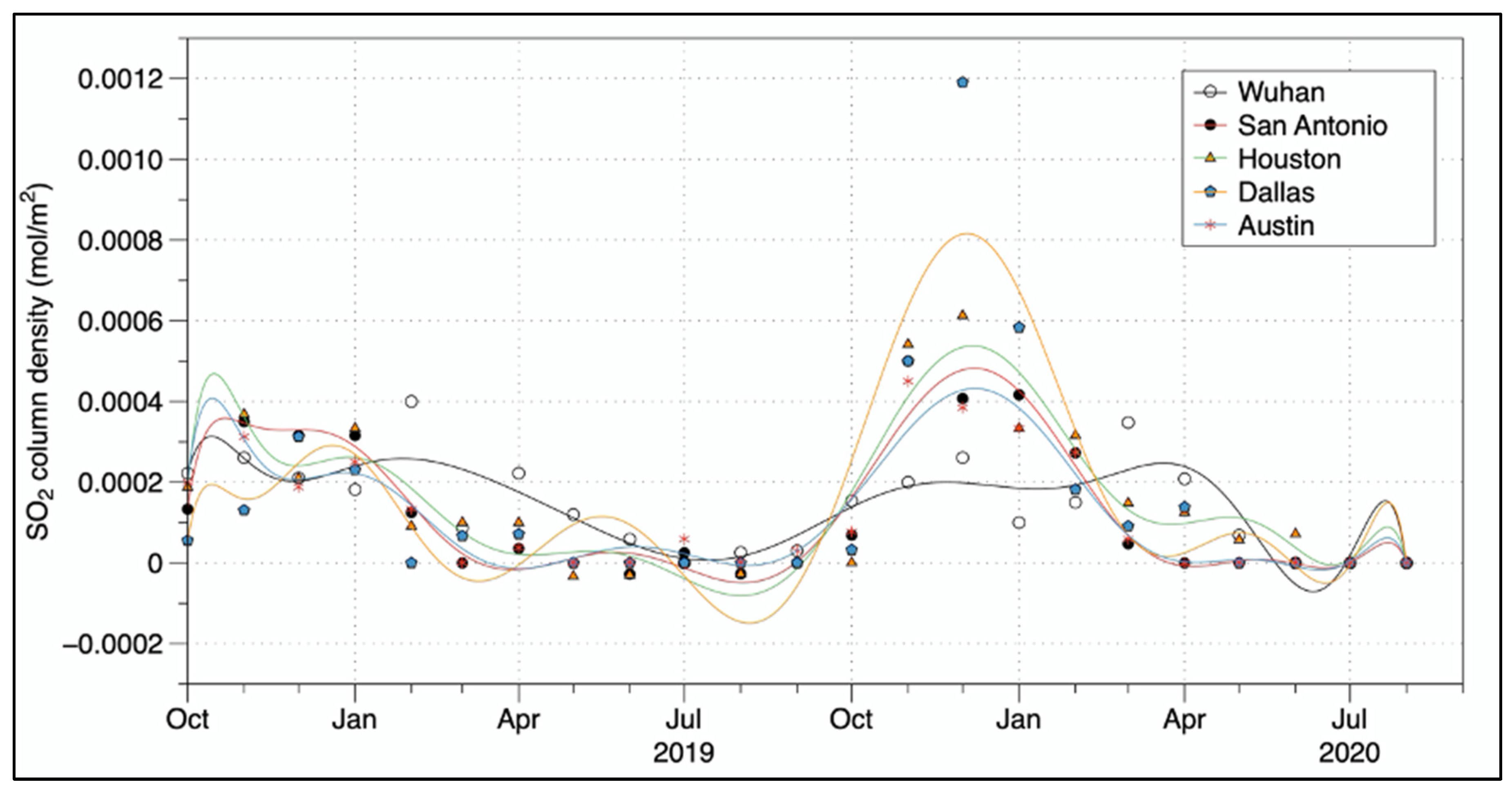
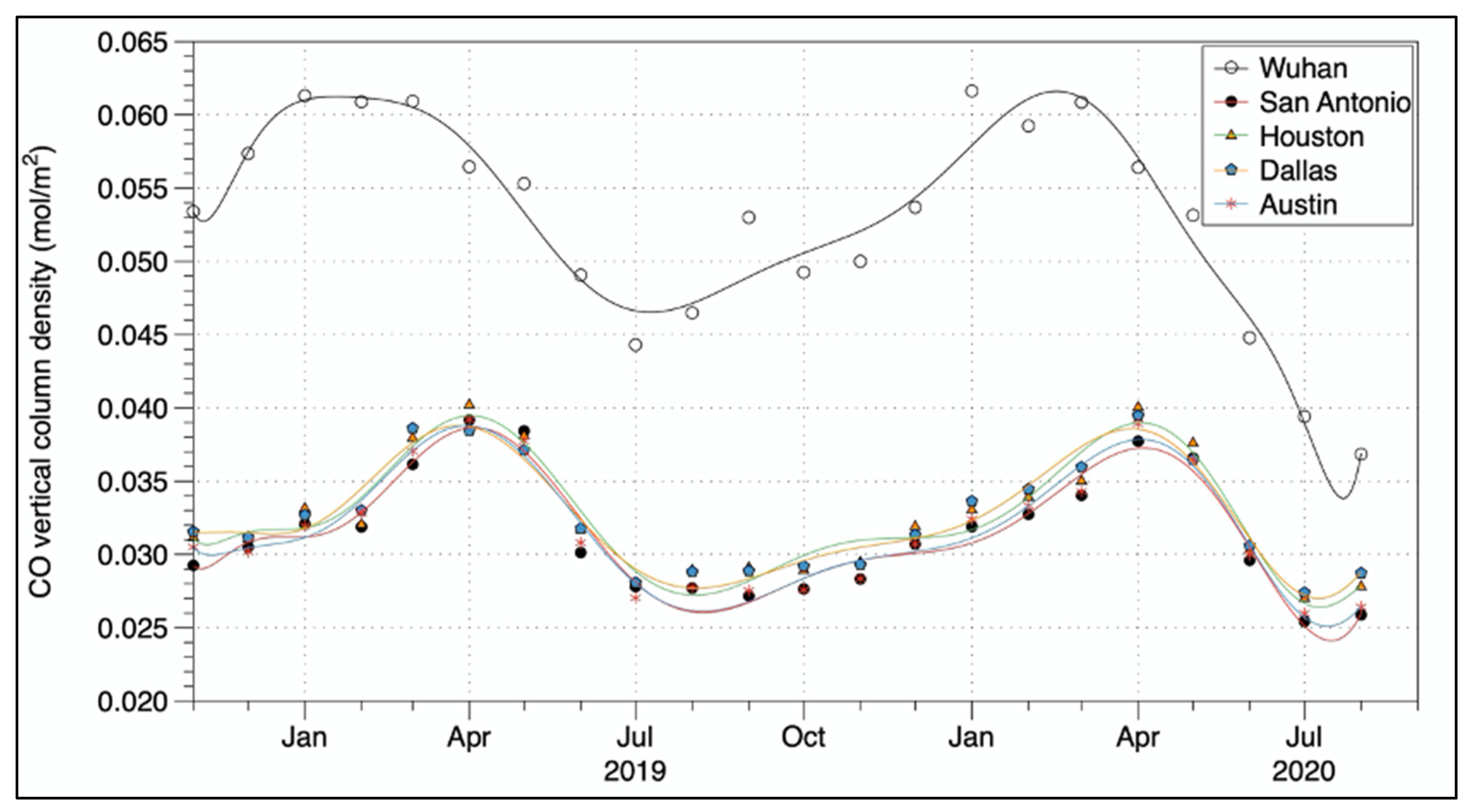
Anthropogenic sources of aerosols are largely attributed to burning fossil fuels, exhaust and combustion of other hydrocarbons. Volatiles that emerge from these activities are typically registered through nitrogen dioxide, sulphur dioxide and carbon monoxide as the compounds oxidize in the atmosphere.
Figure 9,
Figure 10 and
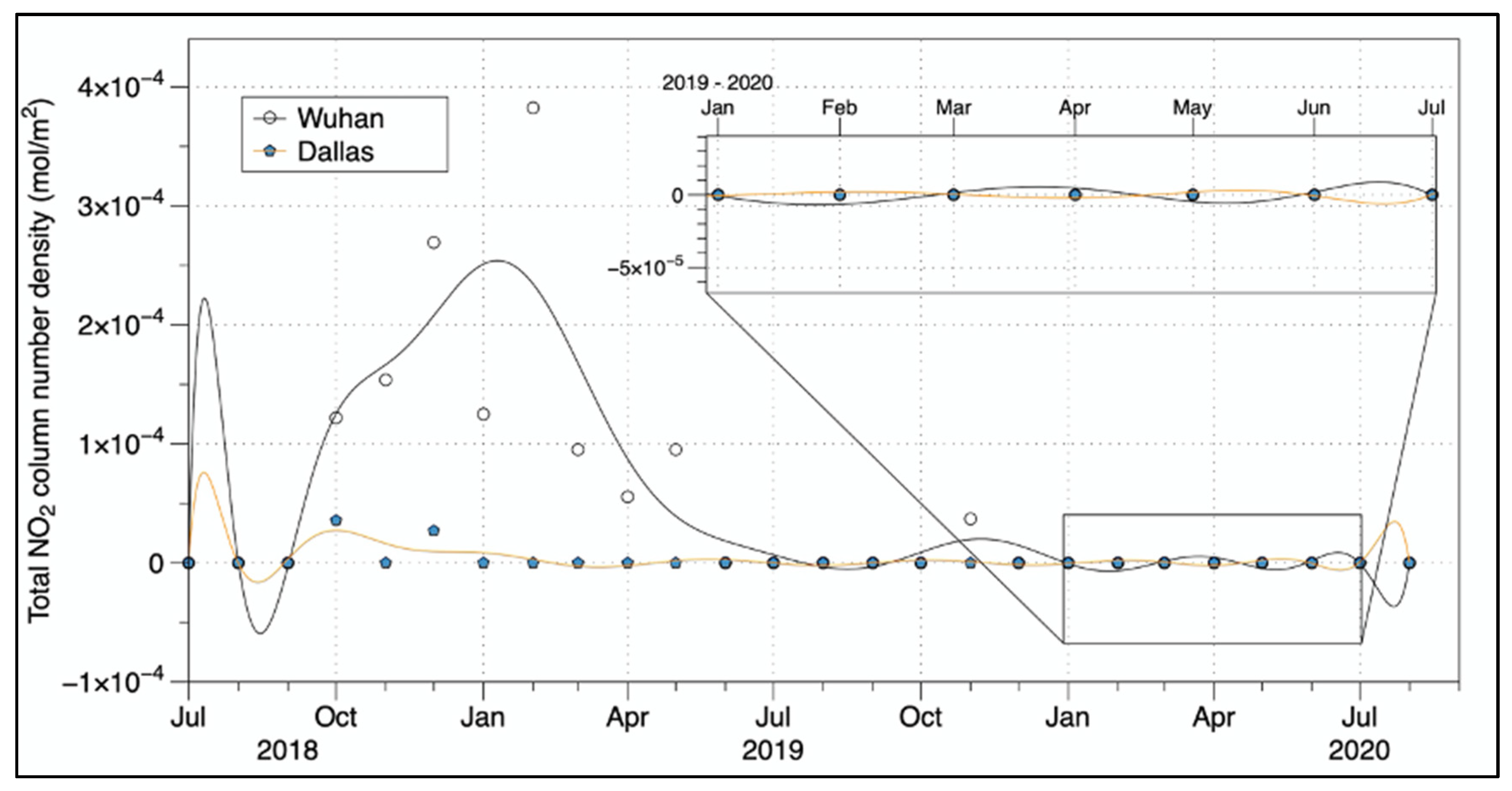
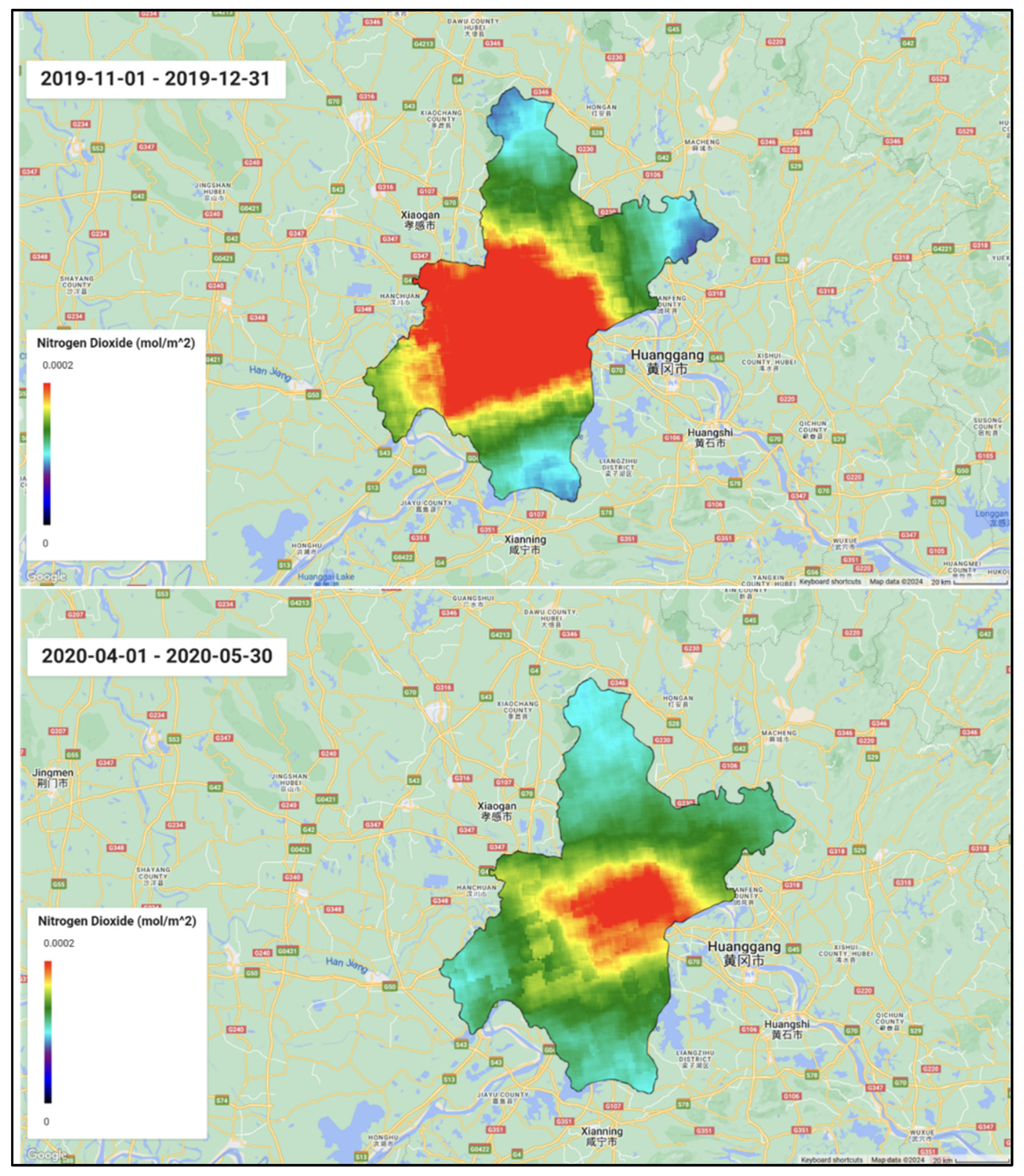
Figure 11 illustrate these compounds over the respective cities. The figures show that Wuhan has higher total nitrogen dioxide and carbon monoxide when compared with any of the Texan cities. The figure shows Wuhan with higher nitrogen dioxide rates well before the pandemic conditions took place.
Nitrogen dioxide levels are particularly high in Wuhan when compared to Texan cities. In fact, the non-log transformed time series of this compound shows negligible values for all the Texan cities, except Dallas. The peak nitrogen dioxide levels in 2019 is several orders of magnitude higher in Wuhan than Dallas. The column density of this compound is dramatically decreased after April 2019, after which the mean fluctuates slightly above zero.
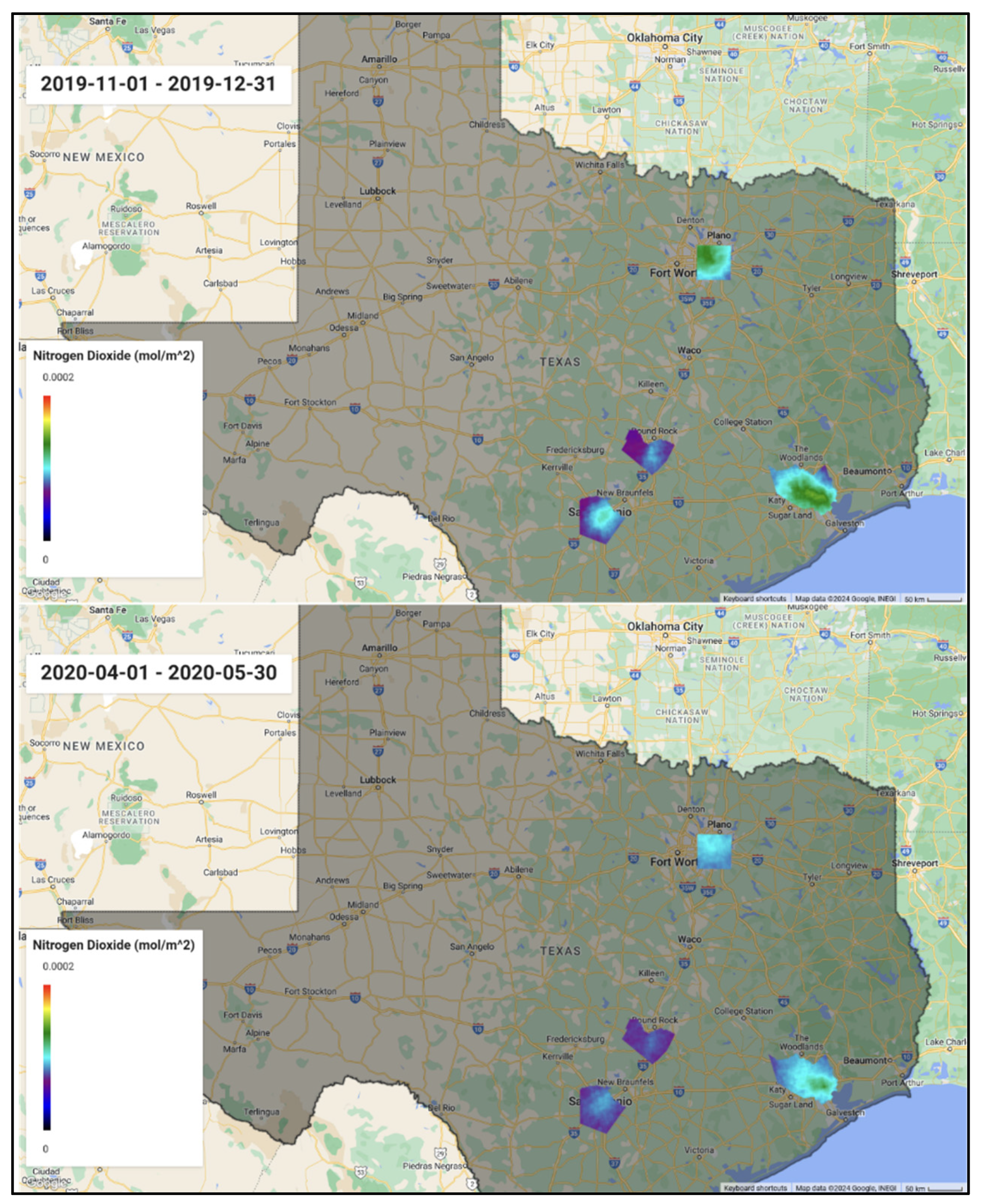
Figure 12 and
Figure 13 show the contrast in nitrogen dioxide levels over Texas in comparison to Wuhan.
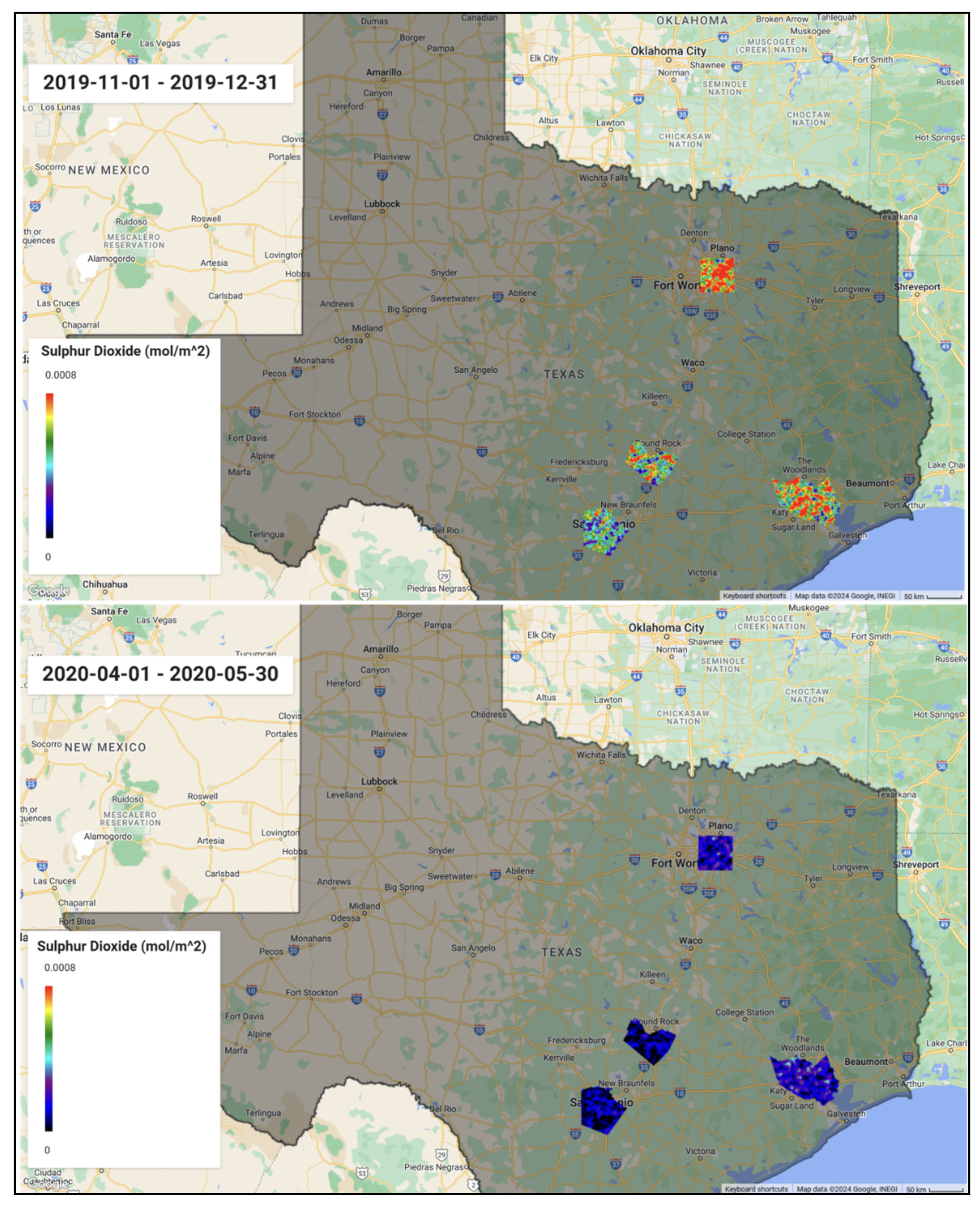
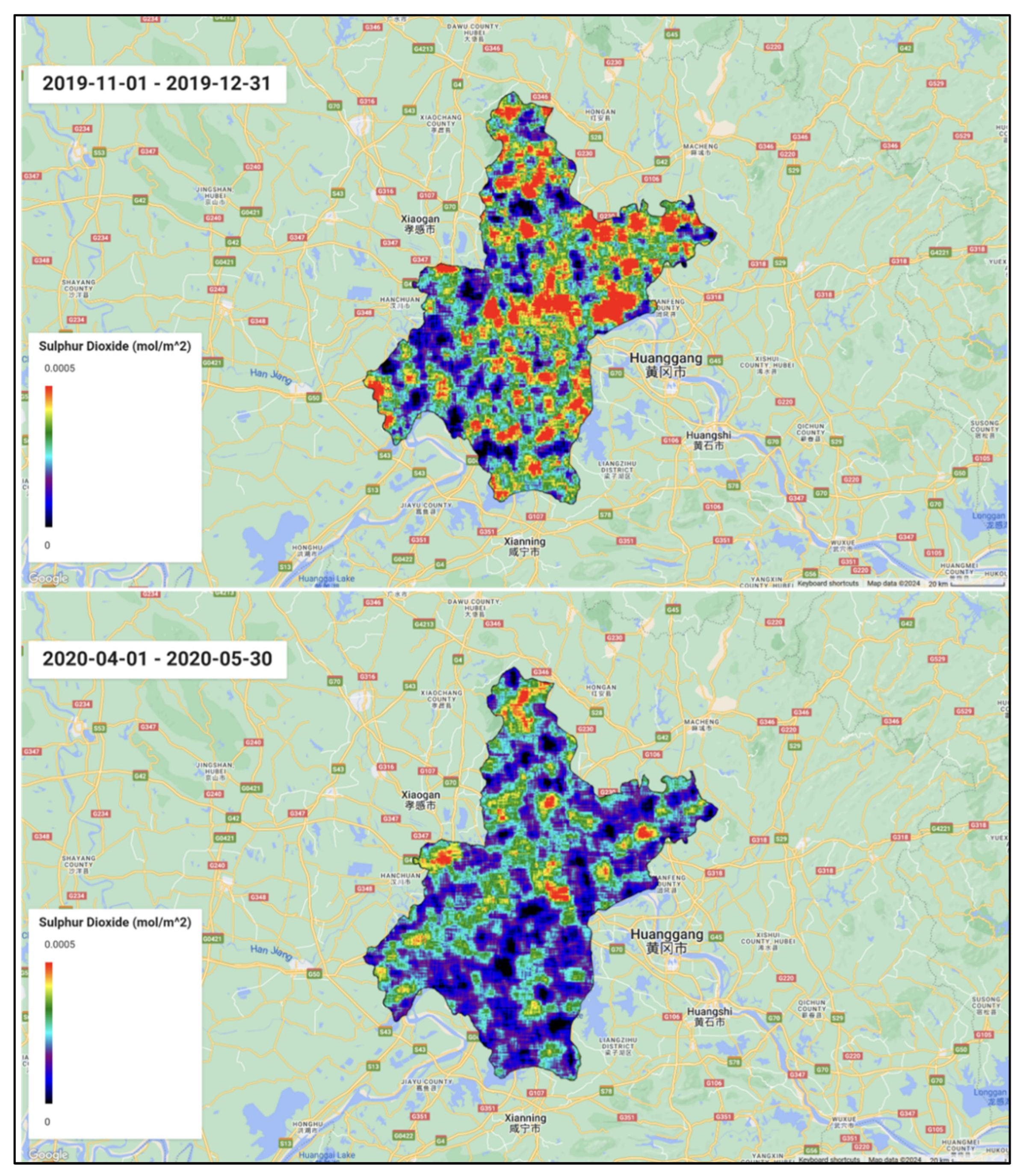
Sulphur dioxide displays a more dynamic relationship and fluctuates more frequently (alternating peaks and troughs) than nitrogen dioxide signatures.
Figure 14 shows that while sulphuric emissions are generally reduced across Texas, Houston and Dallas still display hotspots of sulphur dioxide both before and after the lockdown period.
Figure 15 in contrast, shows higher concentrations of sulphur dioxide scattered across Wuhan, showing no preferential concentration of the compound. Still, there is a marked reduction of sulphur dioxide in the south of Wuhan after lockdown conditions when compared to before.
Wuhan shows that while the compound’s emissions are reduced, hotspots still exist. In December 2019, the very first case of COVID-19 was recorded in China, preceding the lockdown measures taken to curtail its spread. During this time in Texas however, oil production was at its highest in the past 4 years, totaling to 162 million barrels. Sulphur-laden fuel (sour gas) is a ubiquitous source of sulphur dioxide, since Texas is the largest oil producing state in the contiguous United States. The implementation of lockdown conditions saw a downturn in productivity and therefore a decline in the sulphuric compound’s column density (
Figure 10). In the case of China, the sulphur concentrations show its highest reductions in the Southern section of Wuhan.
Carbon monoxide levels in Texas are consistently lower than the levels in Wuhan. Carbon monoxide levels in Wuhan more than 70% higher than Texan cities between February and March 2020 (
Figure 11). However, entering July 2020, the column density of the gas gradually decreases to meet the monoxide levels in Texas.
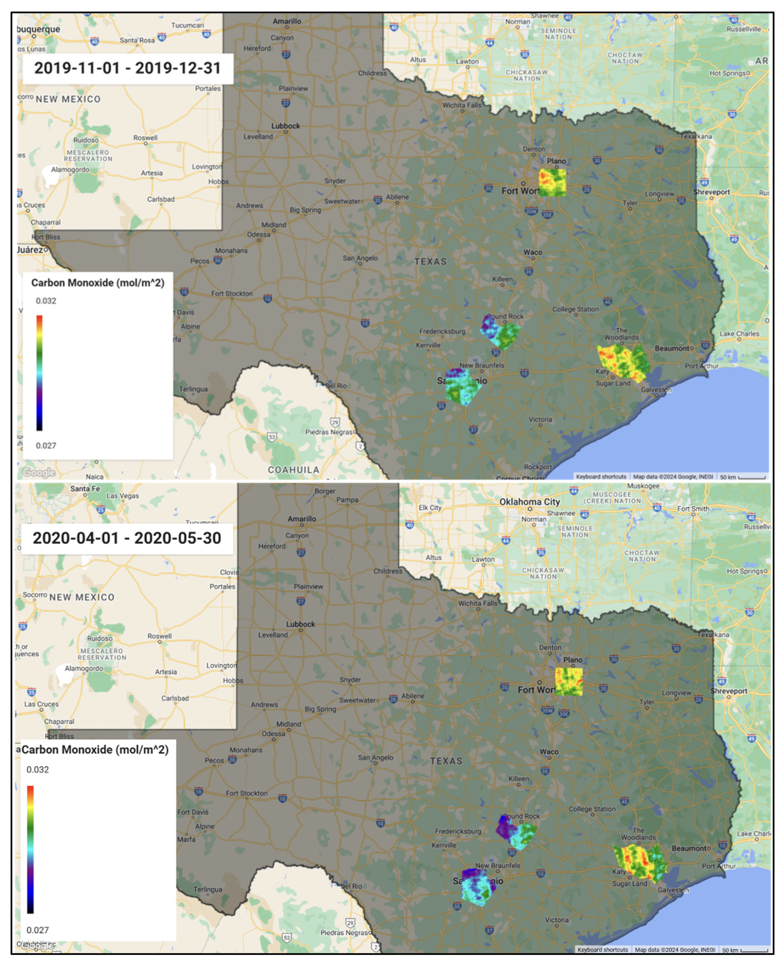
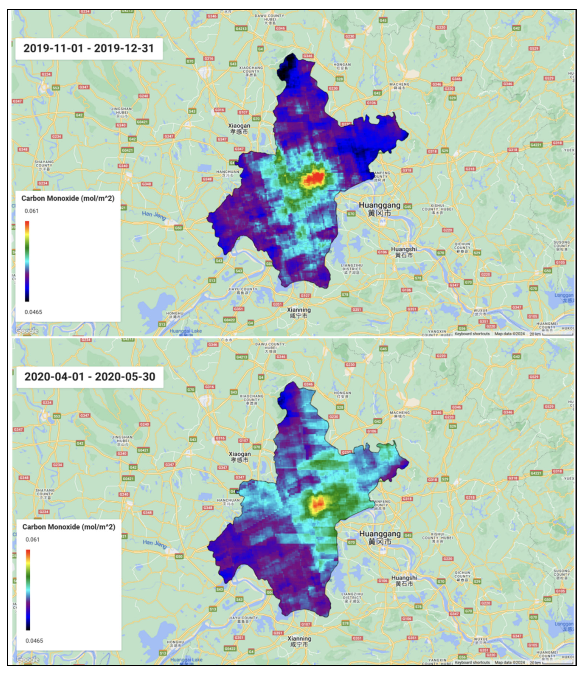
Figure 16 and
Figure 17 show the spatial distribution in the changes in carbon monoxide levels in regions of interest. The case in Texas shows that carbon monoxide levels are higher in Dallas and Houston relative to San Antonio and Austin before shutdown. This trend continues after lockdown conditions are lifted; however, the compound is less concentrated in the forementioned hotspots. Austin and San Antonio show particularly cold spots in the northern sections of the cities. Wuhan shows concentrations more than twice the levels in Texan cities.
Figure 17 shows a defined hotspot point in Wuhan that decreases in size after the global shutdown. There is also a shift in the higher concentrations of carbon monoxide in Wuhan from the south-western to the north-eastern segment of the region.
Conclusions
The global pandemic provides a unique look at atmospheric concentrations with the reduction of human inputs. In an attempt to curtail the spread of the virus, a call for a halt in travel and social interactions was initiated across the globe. In this respect, socio-economic activities stopped, reducing the daily outputs from vehicular exhaust, production and so on. The emissions from imperfect combustion and resultant aerosols have shown marked reductions which can be observed from satellite orbiters.
The general trend shows a downturn in concentrations after lockdown conditions were lifted. While Texas and China are both high industrial regions, the concentrations of the gaseous compounds are generally higher over Wuhan than the selected Texan cities. Though the population size is comparatively higher in Wuhan than the total for all major Texan cities (approximately 19 million and 10 million persons respectively), the collective land area is larger than that of Wuhan. The effect of the shutdown is not immediate, and this is reflected in the shift of the amplitudes of the trends across all compounds.
Changes are observed in all compounds; however, carbon monoxide shows the largest downturn in the short time period. Wuhan maintains a higher concentration of carbon monoxide by several orders of magnitude until the global shutdown. This abrupt change in human activity is immediately reflected in carbon monoxide since its largest outputs are derived from imperfect combustion, typically found in engine mechanisms. Nitrogen dioxide also shows a large change in concentration in Wuhan since the pandemic shutdown. Texas on the other hand, generally did not mirror these abrupt changes. Nevertheless, concentrations of the compounds are found to be higher in Dallas and Houston, where higher populations and densities exist (population densities greater than 2,000 persons per km2 in Dallas and Houston and less than 1,000 persons per km2 in Austin and San Antonio, respectively). Human activity is a driving factor in the concentration of the gases in the troposphere. This is particularly apparent in the lag times of the response of the gas concentrations with respect to the time length of shutdown conditions. Wuhan observed a lockdown period of two months between January and April 2020, while Texas’ lockdown period lasts one month from March to April 2020.
The time allowed for the gases and aerosols to dissipate during a longer shutdown period is apparent with the larger reductions over Wuhan in comparison with Texan cities. In the case of carbon monoxide, the lower limit of its residence time coincides with the length of the lockdown period in Wuhan. The cycling of that compound in the upper atmosphere may account for the much larger reduction in that compound over Wuhan as opposed to Texas. The global shutdown has shown definitively that human activity is a driving force in the proliferation of greenhouse gas emissions into the atmosphere.
Author Contributions
JW processed, analyzed all the data and was the primary author of the paper.
Funding
This work was funded by NASA CAMEE grant#: 80NSSC19M0194.
Acknowledgments
I thank Google Earth Engine and its affiliate platforms for allowing cloud computation of data and analysis as well as Alberto Mestas-Nuñez, Stephen Ackley and Hongjie Xie for their discussions regarding this work.
Conflict of interest
The authors declare no conflict of interests.
References
- Bauwens, M., Compernolle, S., Stavrakou, T., Müller, J., Gent, J., Eskes, H., Levelt, P., A, R., Veefkind, J., Vlietinck, J., Yu, H. and Zehner, C., 2020. Impact of Coronavirus Outbreak on NO 2 Pollution Assessed Using TROPOMI and OMI Observations. Geophysical Research Letters, 47(11).
- Bureau, U.S, 2020. Population. [online] The United States Census Bureau. Available at: <https://www.census.gov/topics/population.html> [Accessed 12 November 2020].
- Burnett, R. and Spadaro, J., 2018. Global Mortality and Long-Term Ambient Exposure to Fine Particulate Matter: A New Relative Risk Estimator. ISEE Conference Abstracts, 2018(1).
- Diamond, M. and Wood, R., 2020. Limited Regional Aerosol and Cloud Microphysical Changes Despite Unprecedented Decline in Nitrogen Oxide Pollution During the February 2020 COVID-19 Shutdown in China. Geophysical Research Letters, 47(17).
- Junge, C., 1974. Residence time and variability of tropospheric trace gases. Tellus, 26(4), pp.477-488.
- Nicola, M., Alsafi, Z., Sohrabi, C., Kerwan, A., Al-Jabir, A., Iosifidis, C., Agha, M. and Agha, R., 2020. The socio-economic implications of the coronavirus pandemic (COVID-19): A review. International Journal of Surgery, 78, pp.185-193.
- Stein Zweers, D.C. TROPOMI ATBD of the UV aerosol index. Royal Netherlands Meteorological Institute; Ministry of Infrastructure and the Environment. 2022, 2.1.0, 9-18.
- Weinstock, B., 1969. Carbon Monoxide: Residence Time in the Atmosphere. Science, 166(3902), pp.224-225.
Figure 1.
Regions of interest in Texas (Austin, Dallas, Houston and San Antonio), USA.
Figure 1.
Regions of interest in Texas (Austin, Dallas, Houston and San Antonio), USA.
Figure 2.
Region of interest in Wuhan, Hubei Province, China.
Figure 2.
Region of interest in Wuhan, Hubei Province, China.
Figure 3.
Water vapor column over the four major Texan cities: Austin, Dallas, Houston and San Antonio and Wuhan, China.
Figure 3.
Water vapor column over the four major Texan cities: Austin, Dallas, Houston and San Antonio and Wuhan, China.
Figure 4.
Cloud albedo over the four major Texan cities: Austin, Dallas, Houston and San Antonio and Wuhan, China.
Figure 4.
Cloud albedo over the four major Texan cities: Austin, Dallas, Houston and San Antonio and Wuhan, China.
Figure 5.
Ozone column density over the four major Texan cities: Austin, Dallas, Houston and San Antonio and Wuhan, China.
Figure 5.
Ozone column density over the four major Texan cities: Austin, Dallas, Houston and San Antonio and Wuhan, China.
Figure 6.
UVAI over the four major Texan cities: Austin, Dallas, Houston and San Antonio and Wuhan, China.
Figure 6.
UVAI over the four major Texan cities: Austin, Dallas, Houston and San Antonio and Wuhan, China.
Figure 7.
UVAI over the four major Texan cities: Austin, Dallas, Houston and San Antonio. Reference times are before shutdown (Nov 1 – Dec 31, 2019) and after (Apr 1 – May 5, 2020).
Figure 7.
UVAI over the four major Texan cities: Austin, Dallas, Houston and San Antonio. Reference times are before shutdown (Nov 1 – Dec 31, 2019) and after (Apr 1 – May 5, 2020).
Figure 8.
UVAI over Wuhan, China. Reference times are before shutdown (Nov 1 – Dec 31, 2019) and after (Apr 1 – May 5, 2020).
Figure 8.
UVAI over Wuhan, China. Reference times are before shutdown (Nov 1 – Dec 31, 2019) and after (Apr 1 – May 5, 2020).
Figure 9.
Nitrogen Dioxide over Dallas, Texas and Wuhan, China. *Other Texan cities were negligible.
Figure 9.
Nitrogen Dioxide over Dallas, Texas and Wuhan, China. *Other Texan cities were negligible.
Figure 10.
Sulphur Dioxide over the four major Texan cities: Austin, Dallas, Houston and San Antonio and Wuhan, China.
Figure 10.
Sulphur Dioxide over the four major Texan cities: Austin, Dallas, Houston and San Antonio and Wuhan, China.
Figure 11.
Carbon Monoxide over the four major Texan cities: Austin, Dallas, Houston and San Antonio and Wuhan, China.
Figure 11.
Carbon Monoxide over the four major Texan cities: Austin, Dallas, Houston and San Antonio and Wuhan, China.
Figure 12.
Nitrogen dioxide over the four major Texan cities: Austin, Dallas, Houston and San Antonio. Reference times are before shutdown (Nov 1 – Dec 31, 2019) and after (Apr 1 – May 5, 2020).
Figure 12.
Nitrogen dioxide over the four major Texan cities: Austin, Dallas, Houston and San Antonio. Reference times are before shutdown (Nov 1 – Dec 31, 2019) and after (Apr 1 – May 5, 2020).
Figure 13.
Nitrogen dioxide over Wuhan, China. Reference times are before shutdown (Nov 1 – Dec 31, 2019) and after (Apr 1 – May 5, 2020).
Figure 13.
Nitrogen dioxide over Wuhan, China. Reference times are before shutdown (Nov 1 – Dec 31, 2019) and after (Apr 1 – May 5, 2020).
Figure 14.
Sulphur dioxide over the four major Texan cities: Austin, Dallas, Houston and San Antonio. Reference times are before shutdown (Nov 1 – Dec 31, 2019) and after (Apr 1 – May 5, 2020).
Figure 14.
Sulphur dioxide over the four major Texan cities: Austin, Dallas, Houston and San Antonio. Reference times are before shutdown (Nov 1 – Dec 31, 2019) and after (Apr 1 – May 5, 2020).
Figure 15.
Sulphur dioxide over Wuhan, China. Reference times are before shutdown (Nov 1 – Dec 31, 2019) and after (Apr 1 – May 5, 2020).
Figure 15.
Sulphur dioxide over Wuhan, China. Reference times are before shutdown (Nov 1 – Dec 31, 2019) and after (Apr 1 – May 5, 2020).
Figure 16.
Carbon monoxide over the four major Texan cities: Austin, Dallas, Houston and San Antonio. Reference times are before shutdown (Nov 1 – Dec 31, 2019) and after (Apr 1 – May 5, 2020).
Figure 16.
Carbon monoxide over the four major Texan cities: Austin, Dallas, Houston and San Antonio. Reference times are before shutdown (Nov 1 – Dec 31, 2019) and after (Apr 1 – May 5, 2020).
Figure 17.
Carbon monoxide over Wuhan, China. Reference times are before shutdown (Nov 1 – Dec 31, 2019) and after (Apr 1 – May 5, 2020).
Figure 17.
Carbon monoxide over Wuhan, China. Reference times are before shutdown (Nov 1 – Dec 31, 2019) and after (Apr 1 – May 5, 2020).
|
Disclaimer/Publisher’s Note: The statements, opinions and data contained in all publications are solely those of the individual author(s) and contributor(s) and not of MDPI and/or the editor(s). MDPI and/or the editor(s) disclaim responsibility for any injury to people or property resulting from any ideas, methods, instructions or products referred to in the content. |
© 2024 by the authors. Licensee MDPI, Basel, Switzerland. This article is an open access article distributed under the terms and conditions of the Creative Commons Attribution (CC BY) license (http://creativecommons.org/licenses/by/4.0/).
