Gap Filling of Missing and Outlier Values of Rotorcraft Flight Data using Multilayer Perceptron

Rotorcrafts operate HUMS for fault diagnosis, but the capabilities of HUMS analysts are important due to the complex mechanical configuration of rotorcraft and the difficulty of analysis. Accordingly, an advanced algorithm is needed to identify faults, and flight data can be used to develop the algorithm. However, flight data contains abnormal or missing data due to problems such as sensor defects, which can be a major problem in algorithm development. Therefore, in this paper, we study a gap filling method using MLP to obtain normal data when there are problems such as abnormal or missing data in rotorcraft flight data. Existing methods typically fill the gap through interpolation or curve fitting using the before and after values of missing data. However, in this study, normal values were estimated using the values of other parameters at the moment of missing or abnormal data occurred. As a result of evaluating the performance of the trained MLP using normal data, it was confirmed that the output of the model well estimates the changing trend of the target. And when abnormal data was applied to the trained model, it was confirmed that point outliers were eliminated and appropriate values were found in the case of missing data.

Keywords:

Subject: Engineering - Aerospace Engineering

1. Introduction

Today, rotorcrafts are used for a variety of purposes, including military and civilian purposes. Rotorcraft have shown a relatively high accident record, at least 2 to 6 times higher than fixed wing aircraft [1] because of the dangerous missions and complex mechanical configurations. Many parts of a rotorcraft are complexly combined with other parts. In particular, engines, transmissions, and rotors that compose the propulsion system are key components that directly affect flight safety [2]. A study of fatal accidents in rotorcraft shows that airworthiness-related accidents of engines, transmissions, and rotors account for 77% of all accidents. The transmission system accounts for approximately 22% and is recognized as a major cause of accidents [3]. Additionally, even if the cause of the accident has not been clearly identified, it is assumed that the transmission and related components are potentially the main cause of the accident [2]. Accordingly, in 1984, the UK CAA (Civil Aviation Authority) insisted on the need to develop a condition monitoring system to prevent rotorcraft accidents, and the development of VHMS (Vibration Health Monitoring System) began in 1989. Afterwards, the flight data monitoring function was added and now forms HUMS (Health and Usage Monitoring System) [1]. HUMS is a device that monitors, acquires, processes, and stores rotorcraft health and usage information, and displays cautions, excesses, and operation history on the PIP (Pilot Interface Panel) [4]. HUMS mainly contributes to ensuring the safety of rotorcraft. From 1990 to 1996, there were 12 accidents involving U.S. Navy and Marine Corps, and five of which were fatal. In a follow-up investigation, it was determined that all accidents could have been prevented if HUMS had been installed [5].

The HUMS of the target rotorcraft is classified into four categories: Airframe, Engine, Transmission, and RTB (Rotor Tracking and Balancing) to diagnose the condition of the aircraft. Monitoring is performed through analysis of CI (Condition Indicator) excesses and changing trends for each system, leading to maintenance such as repair or exchange when necessary. However, HUMS just calculates the CI values and identifies whether the values exceed thresholds, HUMS analysts are responsible for analyzing the changing trends of CIs and determining the need for maintenance. Therefore, the same data may be interpreted differently depending on the experience and capabilities of the HUMS analyst. Additionally, when the CI exceeds the threshold, HUMS analysts request additional flights because additional data of approximately 20 flight hours after the exceedance are needed to analyze changing trend of CI. However, data analysis is difficult because pilots are reluctant to fly the aircraft if alarms due to exceeding the threshold continue to occur. Also, most of the exceedance are spikes and these are not considered faults. And even if the CI values exceed the thresholds continuously, it is judged to be normal if they no longer rise and stabilize. In this case, the threshold values should be adjusted appropriately. However, the values are not updated in real time, and even if updated, the values cannot be applied differently for each unit. Therefore, resetting the thresholds cannot be a fundamental solution.

As a result, in order to analyze CIs and diagnose failures using HUMS, the characteristics and operating environment of each unit should be considered and flight data can be utilized. In fact, HUMS analysts sometimes refer to flight data when analyzing changes in CIs, but there is no automated system to monitor the status of rotorcraft by merging flight data and HUMS data. In summary, a new automated diagnosis system is needed to overcome the ambiguity of judgment in the HUMS data analysis process and reflect the characteristics and operating environment of each unit. Accordingly, our team plans to develop an FDR – HUMS convergence fault diagnosis system based on AI (Artificial Intelligence) and big data.

Prior to system development, it is essential to acquire high-quality and large amounts of flight data to expand from the existing HUMS-based fault diagnosis system to the FDR – HUMS convergence fault diagnosis system. More than 300 parameters are recorded in rotorcraft flight data, including status information of the airframe, engine, transmission and so on. Since these data are generated based on sensors, outliers may occur due to problems such as measurement errors, and sometimes the entire data of some parameters are missing due to problems such as connection errors during the data acquisition process and it can cause problems in developing advanced fault diagnosis algorithms.

Meanwhile, the flight data of the target rotorcraft has sampling rates ranging from 1 to 8hz. In other words, the data in which all variables are recorded simultaneously accounts for only 1/8 of the total. Although in the case of a rotorcraft that has been in operation for a long time and has a lot of data, only 1/8 of the data may be sufficient to develop a data-based AI model, however, if the accumulated data is small, the accuracy of the developed model may be low due to insufficient data. Accordingly, in this paper, we conducted a study to predict missing values due to sensor measurement errors and at the same time interpolate missing rotorcraft flight data due to differences in sampling rates.

Time series data such as flight data are handled in many fields such as weather stations, financial stocks, industrial sensor [6], and various methods are used for data gap filling depending on the data characteristics. For example, simple methods such as linear interpolation, moving average, spline interpolation, Kalman filter [7], as well as more complex models such as radial bases functions, moving least squares, adaptive inverse distance weighted [8], are also used. These simple methods have the disadvantage of low accuracy when interpolating missing data over a relatively long period of time [6]. Additionally, some algorithms can be greatly affected by outliers, and some algorithms cannot be applied if data is missing for the entire operating time.

Recently, data interpolation using ANN (Artificial Neural Network) has also been studied in various fields. Rui Rodrigues [9] has performed gap filling using PhysioNet/Computing in Cardiology Challenge 2010 data. The data was recorded for 10 minutes and one signal was not recorded in the last 30 seconds, and RBM (Restricted Boltzmann Machine) and autoencoder were used to reconstruct the data. As a result of training, the proposed model performed well in reconstruction of signal missing. However, in order to train the model, normally recorded data (9 minutes and 30 seconds in the reference) of some parameters, including missing signals, are required, and it is not applicable if the missing data is not recorded from beginning to end.

J. Pascual-Granado et al. [10] designed and applied the MIARMA (method of interpolation by autoregressive and moving average) model based on the ARMA (autoregressive moving-average) model to fill the gap of the light curves of pulsating stars observed by CoRoT satellite. In the paper, it was confirmed that MIARMA is more suitable for gap filling of light curves compared to linear interpolation and the ARMA interpolation method. However, since flight data can consider various parameters together, the method that considers only one parameter may not be suitable for flight data.

Meteorological data is also one of the fields in which gap filling is being widely studied. According to Coutinho et al. [11], missing data prediction using ANN performed best in many cases [11-14], and in their paper, maximum air temperature and relative air humidity values were predicted using the MLP (Multilayer Perceptron) model. The paper predicted maximum air temperature using maximum air temperature data and predicted relative air humidity using relative air humidity data. In this case, the correlation between input and target is high and a complex model is not required for gap filling. Also, it may not be suitable for flight data because various parameters are not considered as input.

Referring to those papers, this paper performed gap filling of flight data from various flight parameters using MLP. MLP is a representative model of ANN and has shown relatively high performance in references. In chapter 2, flight parameters and valid data for MLP training were identified, and Chapter 3 explained the structure and training process of MLP. And in chapter 4, the performance evaluation of the trained MLP model was conducted using various data, and the conclusions are described in Chapter 5.

2. Identification of Rotorcraft Flight Parameters and Data for MLP Training

2.1. Input and Target Parameters of MLP Model

A total 325 parameters are recorded in the flight data of the target rotorcraft, and the data are recorded at a sampling rate of 1 to 8hz depending on the parameter. Table 1 shows the number of recorded parameters according to the type and sampling rate. Discrete parameters are data that represent the state of the system or data, and INT belongs to binary or multi-class data. HEX parameters are data containing multiple bits in hexadecimal. The continuous parameters are continuous time series data and recorded in INT or FLOAT format. The most common sampling rate is 8hz with 152, followed by 1hz, 4hz, and 2hz.

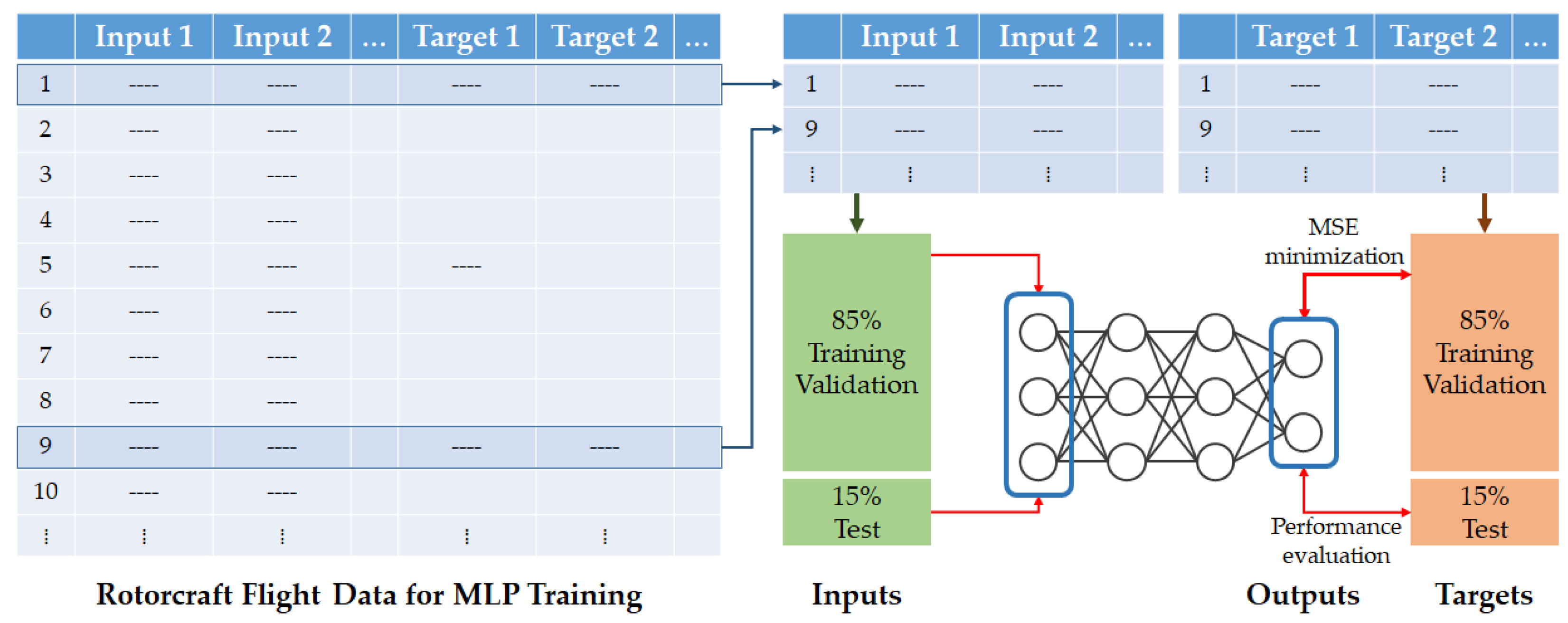
In this paper, only continuous parameters were targeted. Since we want to estimate missing data and at the same time interpolate data for low sampling rate parameters, as shown in Figure 1, parameters recorded at an 8hz sampling rate were selected as input, and the oil pressure and oil temperature of engine and gear box and hydraulic circuit temperature recorded at a sampling rate of 1 and 2hz were selected as targets. These targets correspond to some of the main monitoring targets that are displayed on the PIP (Pilot Interface Panel) when a problem occurs, and are recorded in HUMS exceedance when the values exceed the thresholds. In addition, according to maintenance history, the number of maintenance cases for MGB (Main Gear Box) and TGB (Tail Gear Box) occurs the most, approximately 15% of the total and it was confirmed that most of complaints of gear box were related to oil, such as oil leaks and defective oil temperature sensors. In summary, 61 inputs and 10 targets were selected.

2.2. Identification of Abnormal Data and Construction of Training and Inference Data

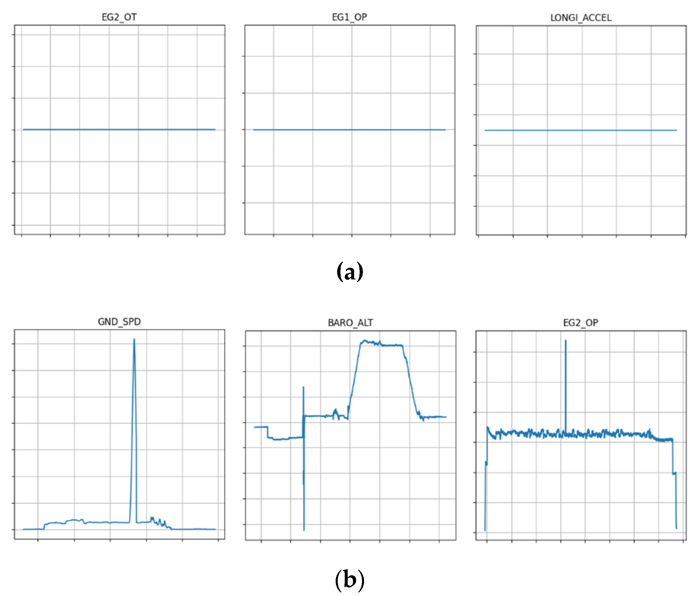
In this study, 587 sortie data from one unit were used to train the MLP model. Among the 587 sorties, data was checked for each sortie to identify abnormal sorties, and it was confirmed that there were 69 cases in which data was not recorded as shown in Figure 2 (a), and there were 37 cases with spikes as shown in Figure 2 (b).

And when checking the number of abnormal data for each parameter, the oil pressure of both engines occurred the most with 69 cases, and abnormal data related to oil accounted for more than 75%, including 8 cases of engine oil temperature and 3 cases of MGB oil pressure.

As a result, 85 sorties had abnormal data and were excluded from training, and 502 sorties were used for MLP training and inference. The number of abnormal data occurrences is 106, but the reason there are 85 abnormal sorties is because there are cases where multiple abnormal data occurred in one sortie. Among normal sorties, 50 sorties, corresponding to 10%, were randomly selected and classified separately to check the inference performance of the trained model, and 452 sortie data were used for MLP training and test. The number of samples in 452 samples is approximately 3.4 million. About 2.38 million samples, corresponding to 70% were used for MLP training, and about 510,000 samples were used for validation and test, respectively. Training, validation, and test data were selected randomly, and the proportion of data used for model training and inference is shown in Figure 3.

3. MLP Model Structure and Training

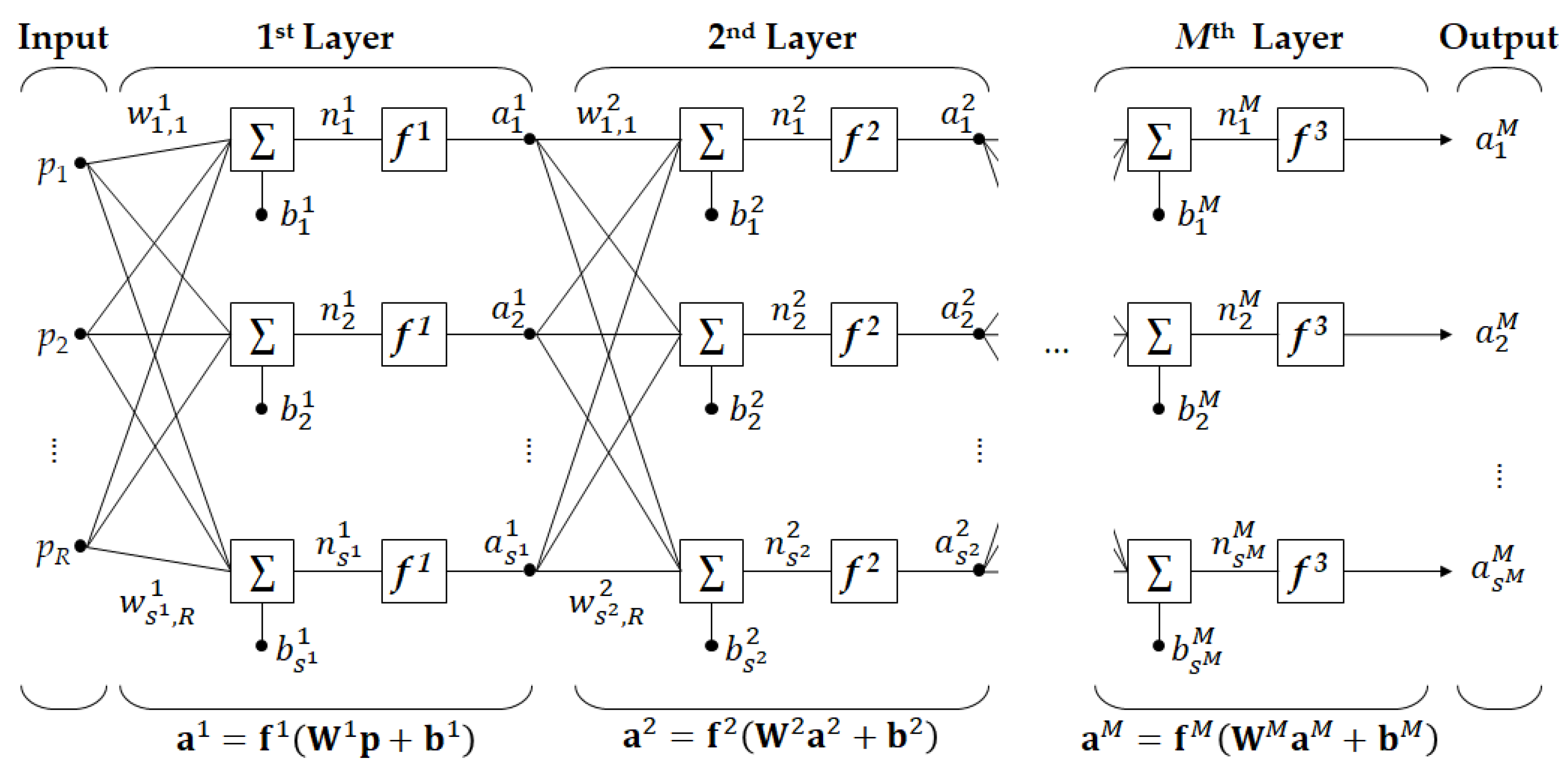
MLP is one of the ANN models and is used for data regression and classification. In this paper, MLP was used as a regression model to estimate target data from input data. The MLP model consists of several layers, and each layer includes neurons and activation functions. Figure 4 shows the structure of a general MLP composed of M layers, and the number of neurons in the i-th layer is sⁱ. The calculation process at each layer is as follows.

The output of the previous layer (input p for the 1st layer) is used as input;
The inputs of the layer are multiplied by the weights;
Biases are added to the calculation results in step 2;
The results of step 3 become inputs to the activation functions;
The outputs of the activation functions become the outputs of the layer;
The outputs of the last layers ultimately become the outputs of the network.

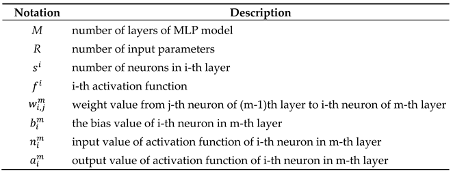
In a regression problem, the number of neurons in the output layer must be equal to the number of target parameters. In this paper, the number of target parameters is 10, so the number of neurons in the output layer is fixed at 10. The calculation process of MLP is the same as Equation (1). The meaning of the notation of each symbol is as shown in Table 2 and follows reference [15].

a^{M} = f^{M} \dots (W^{3} f^{2} (W^{2} f^{1} (W^{1} p + b_{1}) + b_{2}) + b_{3}) + \dots,

(1)

An activation functions are necessary to provide non-linearity to the MLP model, and representative activation functions include sigmoid, tanh, softmax, ReLU, etc. If the number of layers of the MLP is small, training is possible with the sigmoid or tanh function, but as the number of layers increases, such as in deep learning, using the activation functions squashes the characteristics of the data during backpropagation. As a result, training does not work well with the activation functions, so ReLU and its variant activation functions are mainly used in deep learning. The activation function of the hidden layer may vary depending on the given problem, but is generally used in the following order: SELU > ELU > LeakyReLU (and its variants) > ReLU > tanh > logistic [16]. Accordingly, the SELU activation function was used in this paper.

The activation function of the output layer varies depending on the problem to be solved. A linear function is used for regression problems of continuous data, a logistic function is used for binary classification problems, and a softmax activation function is used for multi-classification problems. In this paper, linear was used as the activation function of the output layer to solve the regression problem of continuous data.

Meanwhile, the vanishing gradients problem, in which the gradient becomes smaller as it goes to lower layers, or the exploding gradient problem, in which the gradient becomes larger, may occur during the training process. To alleviate the problem, there are ways to initialize the weights of each layer such as Glorot initialization [17], He initialization [18] and LeCun initialization [19].

Table 3 shows the appropriate initialization strategy according to the activation function [16]. In this paper, LeCun Initialization was applied to the hidden layer using the SELU activation function, and Glorot initialization was applied to the output layer using the linear activation function.

Better results can be expected when the MLP model has multiple hidden layers instead of one [9, 20]. Therefore, in this paper, 5 to 8 layers were configured to find an MLP structure suitable for the given problem, and a parametric study was conducted by combining the number of neurons from 30 to 80. In most cases, using neurons of the same size in all hidden layers can produce the same or better performance as other structures [16], and has the advantage of simplifying the parameters to be tuned in relation to the number of neurons. Therefore, in this paper, the number of neurons in the hidden layer is all the same.

The Adam (adaptive momentum estimation) optimizer [21] was used to train the model. Adam optimizer is widely used in deep learning and has achieved the best performance when training ANN models using flight data [22]. Adam optimizer’s hyper parameters beta1, beta2, and epsilon used default values. The learning rate also used the default value of 0.001.

Meanwhile, the machine learning algorithm does not work well when the scale of the input data is very different. In this case, data normalization is necessary. Data normalization includes a min-max scaler that maps data to a specific range, and a standard scaler that makes the average 0 and the variance 1. In particular, a scaler must be applied to the input data used in this study because flight parameters of different scales are simultaneously used as input to the model. Since the min-max scaler is greatly affected by outliers, the standard scaler was used in this paper. It is generally known that normalization of the target is not necessary [16]. However, if the scales between target parameters are very different, a model may be trained where the large-scale output has high accuracy but the small-scale output has low accuracy [23]. Therefore, in this study, a standard scaler was applied to both input and target, and the scaling formula was developed using only training data (70%). And the formula was applied to the test and inference data. In particular, the reason why test data should not be considered when creating normalization equation is because test data should not be involved in training at all.

Artificial neural network models cause overfitting during the training process. Overfitting occurs when the model has very high accuracy only for the given training data. In other words, an overfitted model has a very low training error, but when given unseen data such as test data, it has a very large error, that is, it is a non-generalized model. Accordingly, algorithms such as L2 regularization, dropout, and early stopping were designed as methods to prevent overfitting. In order to apply the early stopping algorithm, validation data must be configured separately. Therefore, it is difficult to apply the algorithm when there is insufficient data, but when there is sufficient data, it is worth considering first because training can be terminated quickly. In this paper, since the number of samples that can be used for training is approximately 3.4 million, it was judged that validation data could be sufficiently formed, and early stopping was applied.

In order to implement the early stopping algorithm, approximately 15% of the data consists of validation data, and after each training epoch, the validation loss is calculated using the validation data. And if the loss continues to increase beyond a given opportunity, the model parameters with the smallest loss are finally selected. The given opportunity is called patience, and in this paper, 20 was used based on the author’s experience. Table 4 summarizes the model and hyper parameter information used for training.

The memory capacity of the server used for training was approximately 1TB, and one H100 GPU was used. It took about 40 to 50 seconds for one epoch to be performed on the server.

4. Performance Evaluation of Trained MLP Model

4.1. Performance Evaluation Using Test Data

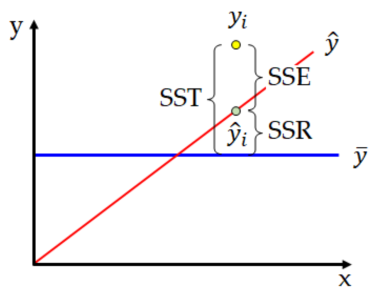
In this section, the performance of the trained MLP model was verified using test data that was not used for training. A representative indicator that evaluates the predictive ability of a regression model is the coefficient of determination R², which means how much the outputs calculated through the regression explain the targets. The meaning and formula of the coefficient of determination are shown in Figure 5 and Equation (2).

However, the coefficient of determination tends to increase as the number of training data and independent variables increases, regardless of the model prediction ability. To complement the problem, this paper used the Adjusted-R² as a performance indicator. The indicator expressed by additionally considering the sample size and number of independent variables to compensate for problems with the coefficient of determination and is shown in Equation (3). In the equation, n is number of samples and p is the number of input parameters.

R^{2} = \frac{S S R}{S S T} = \frac{{Σ ({\hat{y}}_{i} - \bar{y})}^{2}}{{Σ (y_{i} - \bar{y})}^{2}},

(2)

R_{a d j}^{2} = 1 - \frac{(n - 1)}{(n - p)} (1 - R^{2})

(3)

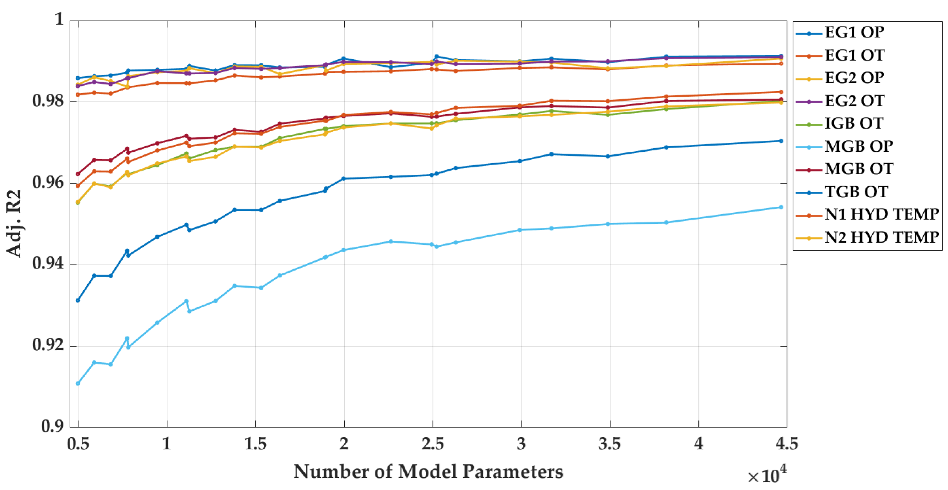
Table 5 shows the number of model parameters and Adjusted-R² according to MLP structures. Model parameters refer to weight and bias, and as the number of layers and neurons increases, the number of model parameters to train also increases. According to Table 5 and Figure 6, it can be seen that the Adjusted-R² increases as the number of model parameters increases. This means that as the complexity of the MLP model increases, the non-linear relationship between inputs and targets can be predicted well, and it suggests that increasing the number of model parameters is likely to further improve accuracy.

Figure 7 is a comparison between the outputs calculated by inputting test data into the trained 8 layers and 80 neurons MLP and targets. In the figure, the x-axis means target and the y-axis means output. The more data is distributed on a virtual straight line with a slope of 1, the more accurately the model estimates the targets. Most of the engine OP (oil pressure) and OT (oil temperature) data are close to the shape of a straight line with a slope of 1, and the coefficient of determination is about 0.99. However, gearbox and hydraulic circuit fluid temperature data are relatively inaccurate, so it can be seen that the points are relatively widely distributed. This is because there are many engine-related parameters in the input, so the target related to the engine can be estimated well, but there are almost no parameters related to gearbox and hydraulic circuit.

4.2. Performance Evaluation Using Normal Inference Data

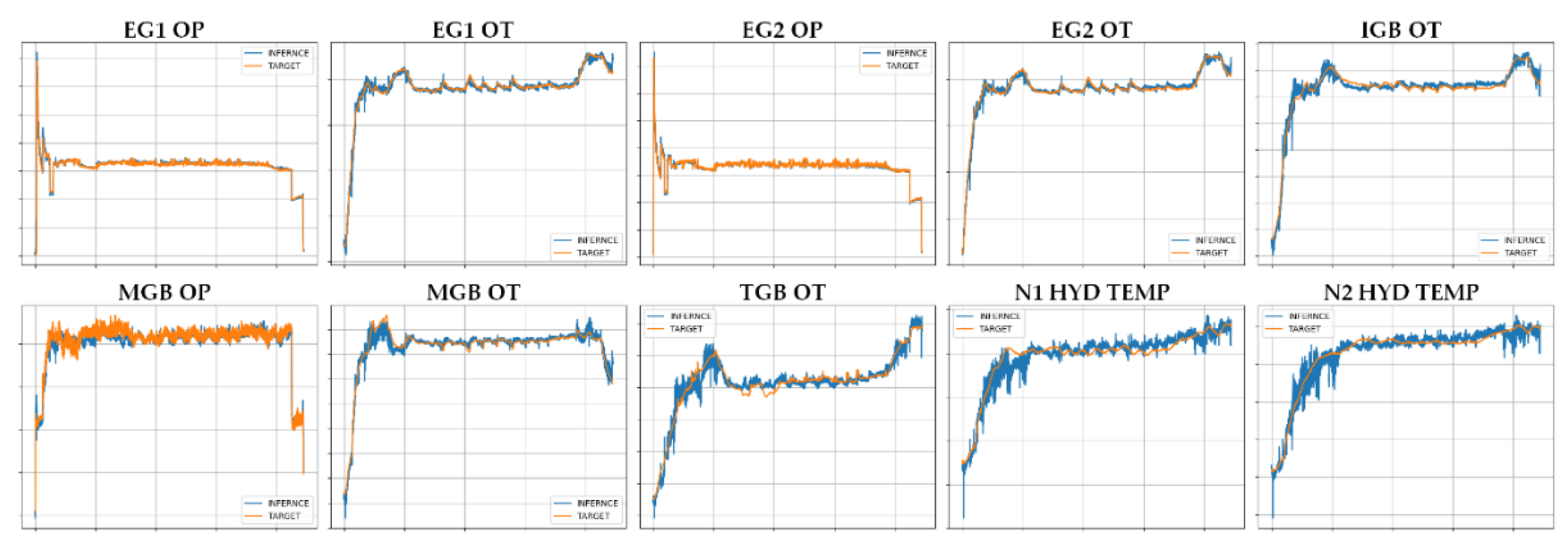
In this section, we evaluated the performance of the trained model using inference data (50 sorties inference data in Figure 3) that has never been used for training. The evaluation was conducted on a model with 8 layers and 80 neurons.

Figure 8 representatively shows the inference results of random sorties among 50 sorties. In the figure, the x-axis is time, and the y-axis is the values of each parameter. And the blue lines are the output of the trained model, and the red lines are the actual recorded targets. In the case of the engine that produced relatively good results in the previous section, it was confirmed that actual data can be estimated well even through inference. Although the gearbox and hydraulic circuit fluid temperature cannot estimate values as accurately as the engine, it can be confirmed that the changing trend of the data can be followed.

In order to increase the accuracy of the parameters, it seems necessary to eliminate input parameters that cause high frequencies in the output through data analysis or apply a filter to the output.

4.3. Performance Evaluation Using Abnormal Inference Data

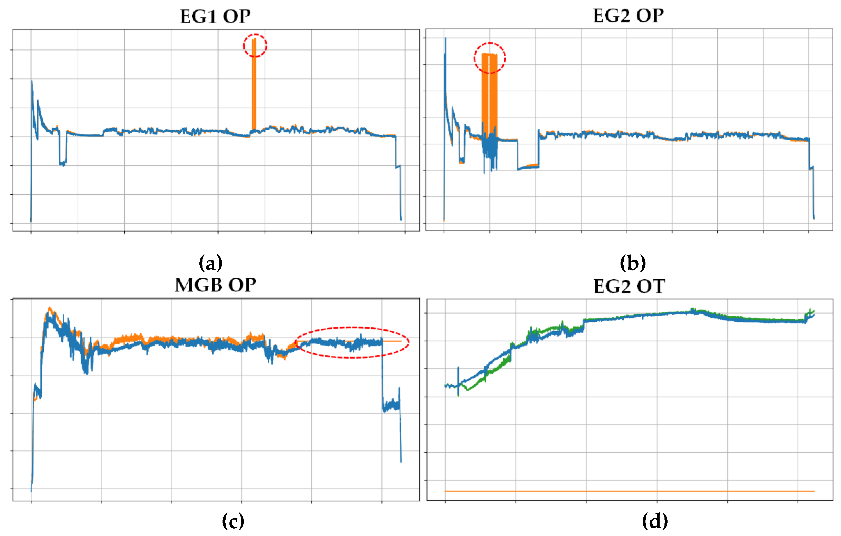
As shown in Figure 2, spike abnormal data and missing data are representative abnormal data. In this section, we observed the outputs when abnormal sortie data was input into the trained MLP. For testing, an MLP trained with a structure of 8 layers and 80 neurons was used. Figure 9 shows the inference results of arbitrary abnormal sorties. The red lines are the actual recorded flight data, and the blue lines are the outputs of the trained MLP.

Figure 9 (a) shows that point outliers occurred in the raw data of engine 1 oil pressure, but there were no outliers in the inference results. And, except for the outliers, it can be confirmed that the remaining data infers the target data well. In Figure 9 (b), for the oil pressure of engine 2, it can be seen that while the raw data showed large spike-like outliers, the inference results showed that the degree of anomaly decreased sharply. In the raw data in Figure 9 (c), MGB oil pressure was not recorded in the latter part of the sortie. On the other hand, the inference result outputs MGB oil pressure, and the changing trend of the output data was confirmed to be similar to other normal sorties (see MGB OP result in Figure 8). Figure 9 (d) shows that although raw data for oil temperature of engine 2 was not recorded at all, the MLP generated data. In the figure, the green line represents the oil temperature of engine 1. In normal data, engine 1 oil temperature and engine 2 oil temperature have a high correlation coefficient (0.934), so their values and changing trends should be similar. In the figure, the values and changing trends of the two oil temperatures are quite similar, so it can be assumed that the data generated by the trained MLP model well reflects the actual flight situation.

5. Conclusions

In this study, prior to developing the rotorcraft FDR-HUMS convergence fault diagnosis algorithm, rotorcraft flight data was analyzed, and an MLP-based gap filling model was trained and applied to process abnormal and missing data. MLP models were trained using normal data, and performance evaluation was performed using test data. As a result of the test, it was confirmed that the engine-related data was estimated well, and the gearbox and hydraulic circuit were relatively inaccurate, but showed a high Adjusted-R² score of over 0.95. This means that the trained model can estimate targets well.

Next, inference of the trained model was performed using sorties that were not used in MLP model training and test. In the case of the engine, inference results were quite accurate and gearbox and hydraulic circuit were following the changing trends of targets well. It is presumed that some high frequency input variables affect the output, and there are ways to eliminate the relevant input parameters through data analysis or apply a filter to the output.

Finally, the model’s inference results were observed for abnormal sortie data. When applying sortie data where spike noises occurred, the inference results of the model confirmed that spikes did not occur while estimating the overall targets well. This means that even if a problem occurs in a specific sensor and abnormal data appears, normal data can be obtained through the model if other sensors are normal. Additionally, it was confirmed that the MLP model can estimate values even when data is not recorded for a certain section or for the entire flight. Although accurate performance evaluation is impossible because there is no target data, when compared with data from other normal sorties or with other parameters with a high correlation, the values and changing trends were quite similar and it was confirmed that the model was reliable.

In developing a fault diagnosis algorithm, it is of course important to accurately predict values, but it is more important to erase abnormal data and analyze data changing trends. Therefore, the developed model is expected to be helpful in gap filling of flight data when developing an advanced fault diagnosis algorithm.

Author Contributions

Conceptualization, S.H.J. and D.K.; methodology, Y.L.; software, I.L.; validation, J.H.K., Y.Y.H.; formal analysis, S.H.J.; investigation, D.K.; resources, I.L.; data curation, Y.L.; writing—original draft preparation, S.H.J.; writing—review and editing, S.H.J.; visualization, S.H.J.; supervision, J.H.K.; project administration, Y.L.; funding acquisition, Y.Y.H. All authors have read and agreed to the published version of the manuscript.

Funding

This research was conducted with support from KRIT (Korea Research Institute for defense Technology planning and advancement) with funding from the government (Defense Acquisition Program Administration) in 2022. (KRIT-CT-22-081, Weapon System CBM+ Research Center)

Data Availability Statement

Restrictions apply to the availability of these data. Data were obtained from the Republic of Korea Ministry of National Defense.

Conflicts of Interest

The authors declare no conflicts of interest.

References

Kim, O.C.; Kim, J.W.; Lee, J.H.; Jo, S.H.; Huh, S.J.; Shin, S.M. Health and Usage Monitoring System Development for Rotorcraft. KSAS 2016 Fall Conference, Jeju, Republic of Korea, 16-18 Nov. 2016.
Lee, S.M.; Hwang, J.S. A Way to Perform a Helicopter PFAT by KUH Case Study. Journal of The Korean Society for Aeronautical and Space Sciences 2013, 41, 994-1001. [CrossRef]
Astridge, D.G. Helicopter Transmissions – Design for Safety and Reliability. Proceedings of the Institution of Mechanical Engineers, Part G: Journal of Aerospace Engineering 1989, 203, 123-138. [CrossRef]
Jung, H.S. A Study for Helicopter’s Health and Usage Monitoring System Efficient Operation – Focusing on the KUH-1 -. Master’s degree, Kongju National University, Gongju-si, Republic of Korea, Feb. 2012.
Kim, O.C.; Ryu, J.B. Application of HUMS System for KHP. Autumn Annual Conference of The Institute of Electronics and Information Engineers, Cheongju-si, Republic of Korea, 3 Nov. 2006.
Sarafanov, M.; Nikitin, N.O.; Kalyuzhnaya, A.V. Automated Data-driven Approach for Gap Filling in the Time Series using Evolutionary Learning. 16th International Conference on Soft Computing Models in Industrial and Environmental Applications (SOCO 2021), Bilbao, Spain, 22-24 Sep. 2021. [CrossRef]
Lepot, M.; Aubin, J.-B.; Clemens, F.H.L.R. Interpolation in Time Series: An Introductive Overview of Existing Methods, Their Performance Criteria and Uncertainty Assessment. Water 2017, 9, 796. [CrossRef]
Ding, Z.; Mei, G.; Cuomo, S.; Li, Y.; Xu, N. Comparison of Estimating Missing Values in IoT Time Series Data Using Different Interpolation Algorithms. Int J Parallel Prog 2020, 48, 534-548. [CrossRef]
Rodrigues, R. Filling in the Gap: A General Method Using Neural Networks. 2010 Computing in Cardiology, Belfast, Northern Ireland, 26-29 Sep. 2010.
Pascual-Granado, J.; Garrido, R.; Suárez, J.C. MIARMA: A Minimal-Loss Information Method for Filling Gaps in Time Series. A&A 2015, 575, A78 1-8. [CrossRef]
Coutinho, E.R.C.; da Silva, R.M.; Madeira, J.G.F.; Coutinho, P.R.O.S.; Boloy, R.A.M.; Delgado, A.R.S. Application of Artificial Neural Networks (ANNs) in the Gap Filling of Meteorological Time Series. Revista Brasileira de Meteorologia 2018, 33, 317-328. [CrossRef]
Bustami, R.; Bessaih, N.; Bong, C.; Suhaili, S. Artificial Neural Network for Precipitation and Water Level Predictions of Bedup River. IAENG International Journal of Computer Science 2007, 34.
Maqsood, I.; Khan, M.R.; Abraham, A. An Ensemble of Neural Networks for Weather Forecasting. Neural Comput & Applic 2004, 13, 112-122. [CrossRef]
Olcese, L.E.; Palancar, G.G.; Toselli, B.M. A Method to Estimate Missing AERONET AOD Values based on Artificial Neural Networks. Atmospheric Environment 2015, 113, 140-150. [CrossRef]
Hagan, M.T.; Demuth, H.B.; Beale, M.H; Jesús, O.D. Neural Network Design, 2nd ed.; Martin Hagan: Stillwater, U.S., 2014.
Géron, A. Hands-On Machine Learning with Scikit-Learn, Keras, and TensorFlow, 2nd ed.; O’Reilly Media, Inc.: Sebastopol, U.S., 2019.
Glorot, X.; Bengio, Y. Understanding the Difficulty of Training Deep Feedforward Neural Networks. Proceedings of the Thirteenth International Conference on Artificial Intelligence and Statistics, Sardinia, Italy, 13-15 May 2010.
He, K.; Zhang, X.; Ren, S.; Sun, J. Delving Deep into Rectifiers: Surpassing Human-Level Performance on ImageNet Classification. 2015 IEEE International Conference on Computer Vision (ICCV), Santiago, Chile, 7-13 Dec. 2015. [CrossRef]
Lecun, Y.A.; Bottou, L.; Orr, G.B.; Müller, K.-R. Efficient BackProp. Neural Networks: Tricks of the Trade; Montavon, G., Müller, K,-R, Orr, G.,B., Eds.; Springer: Berlin, Germany, 2002; Volume 7700, pp. 9-48. [CrossRef]
Bengio, Y.; Lecun, Y. Scaling Learning Algorithms toward AI. Large-Scale Kernel Machines; Bottou, L., Chapelle, O., DeCoste, D., Weston, J., Eds.; The MIT Press: Location, Country, 2007. [CrossRef]
Kingma, D.P.; Ba, J.L. ADAM: A Method for Stochastic Optimization. arXiv 2014, arXiv:1412.6980. [CrossRef]
Jeong, S.H.; Park, E.G.; Cho, J.Y.; Kim, J.H. Development of Automatic Hard Landing Detection Model using Autoencoder. International Journal of Aeronautical and Space Sciences 2023, 24, 778-791. [CrossRef]
Jeong. S.H.; Lee, K.B.; Ham, J.H.; Kim, J.H.; Cho, J.Y. Estimation of Maximum Strains and Loads in Aircraft Landing using Artificial Neural Network. International Journal of Aeronautical and Space Sciences 2019, 21, 117-132. [CrossRef]

Figure 1. Flight data of rotorcraft and MLP training.

Figure 2. Examples of abnormal data: (a) Data is not recorded for the entire sortie; (b) Spikes.

Figure 3. Proportion of data used for MLP training and inference.

Figure 4. Structure of MLP model.

Figure 5. Schematic of determination coefficient.

Figure 6. Relationship between number of model parameters and Adjusted-R².

Figure 7. Target and output plot of test data.

Figure 8. Inference results. The blue lines are output of trained MLP and red lines are target data.

Figure 9. Inference results of abnormal sorties. The red lines are raw data, and the blue lines are inference results: (a) Inference results for spike abnormal sortie data of engine 1 oil pressure; (b) Inference results for spike abnormal sortie data of engine 2 oil pressure; (c) Inference results for some missing data of MGB oil pressure; (d) Inference results for all missing data sortie of engine 2 oil temperature. The green line corresponds to raw data of engine 1 oil temperature.

Table 1. Number of parameters depending on data type and sampling rate.

Sampling Rate			1hz	2hz	4hz	8hz
Type of Data	Discrete	INT	40	3	7	36
	Discrete	HEX	10	18	11	53
	Continuous	INT	21	2	7	11
	Continuous	FLOAT	16	16	22	52
Total			87	39	47	152

Table 2. Notation and description of MLP structure.

Table 3. Weight initialization for each type of activation function.

Initialization	Activation functions
Glorot	None, tanh, logistic, softmax
He	ReLU and variants
LeCun	SELU

Table 4. Model and hyper parameters of MLP.

Model & Hyper Parameters		Value
Number of layers		5 to 8
Number of neurons in hidden layers		30 to 80
Loss function		MSE
Normalization		StandardScaler
Regularization		Early stopping
Patience		20
Epochs		1,000
Batch size		128
Activation functions	hidden layers	SELU
Activation functions	output layer	Linear
Kernel Initializers	hidden layers	LeCun
Kernel Initializers	output layer	Glorot
Adam Optimizer	beta1	0.9
	beta2	0.999
	epsilon	1e-7
	learning rate	0.001

Table 5. Number of model parameters and Adjusted-R² according to MLP structures.

Layers	Neurons	Number of Model Parameters	EG1 OP	EG1 OT	EG2 OP	EG2 OT	MGB OP	MGB OT	IGB OT	TGB OT	N1 HYD TEMP	N2 HYD TEMP
5	30	4,960	0.986	0.982	0.984	0.984	0.911	0.962	0.955	0.931	0.959	0.955
6	30	5,890	0.986	0.982	0.986	0.985	0.916	0.966	0.960	0.937	0.963	0.960
7	30	6,820	0.987	0.982	0.985	0.984	0.916	0.966	0.959	0.937	0.963	0.959
8	30	7,750	0.987	0.984	0.984	0.986	0.922	0.968	0.963	0.943	0.966	0.963
5	40	7,810	0.988	0.984	0.986	0.986	0.920	0.968	0.962	0.942	0.965	0.962
6	40	9,450	0.988	0.985	0.987	0.988	0.926	0.970	0.964	0.947	0.968	0.965
7	40	11,090	0.988	0.985	0.988	0.987	0.931	0.972	0.967	0.950	0.970	0.967
5	50	11,260	0.989	0.985	0.988	0.987	0.929	0.971	0.966	0.949	0.969	0.965
8	40	12,730	0.988	0.985	0.987	0.987	0.931	0.971	0.968	0.951	0.970	0.967
6	50	13,810	0.989	0.986	0.989	0.988	0.935	0.973	0.969	0.953	0.972	0.969
5	60	15,310	0.989	0.986	0.989	0.988	0.934	0.973	0.969	0.953	0.972	0.969
7	50	16,360	0.988	0.986	0.987	0.988	0.937	0.975	0.971	0.956	0.974	0.970
8	50	18,910	0.989	0.987	0.989	0.989	0.942	0.976	0.973	0.958	0.975	0.972
6	60	18,970	0.989	0.987	0.988	0.989	0.942	0.976	0.973	0.959	0.975	0.972
5	70	19,960	0.991	0.987	0.989	0.990	0.944	0.977	0.974	0.961	0.977	0.974
7	60	22,630	0.989	0.988	0.990	0.990	0.946	0.977	0.975	0.962	0.978	0.975
6	70	24,930	0.990	0.988	0.990	0.989	0.945	0.976	0.975	0.962	0.977	0.973
5	80	25,210	0.991	0.988	0.989	0.990	0.944	0.976	0.975	0.962	0.977	0.974
8	60	26,290	0.990	0.988	0.990	0.989	0.945	0.977	0.975	0.964	0.979	0.976
7	70	29,900	0.990	0.988	0.990	0.989	0.949	0.979	0.977	0.965	0.979	0.976
6	80	31,690	0.991	0.988	0.990	0.990	0.949	0.979	0.978	0.967	0.980	0.977
8	70	34,870	0.990	0.988	0.988	0.990	0.950	0.979	0.977	0.967	0.980	0.978
7	80	38,170	0.991	0.989	0.989	0.991	0.950	0.980	0.978	0.969	0.981	0.979
8	80	44,650	0.991	0.989	0.991	0.991	0.954	0.981	0.980	0.970	0.982	0.980

Disclaimer/Publisher’s Note: The statements, opinions and data contained in all publications are solely those of the individual author(s) and contributor(s) and not of MDPI and/or the editor(s). MDPI and/or the editor(s) disclaim responsibility for any injury to people or property resulting from any ideas, methods, instructions or products referred to in the content.

© 2024 by the authors. Licensee MDPI, Basel, Switzerland. This article is an open access article distributed under the terms and conditions of the Creative Commons Attribution (CC BY) license (http://creativecommons.org/licenses/by/4.0/).

Copyright: This open access article is published under a Creative Commons CC BY 4.0 license, which permit the free download, distribution, and reuse, provided that the author and preprint are cited in any reuse.

MDPI Initiatives

Important Links

Choose an area of interest and we will send you notifications of new preprints at your preferred frequency.

Disclaimer