1. Introduction
Particle organic carbon (POC) plays a crucial role in the oceanic carbon cycle, bridging surface primary production with deep sea and sedimentation processes [
1]. Originating from marine biological metabolism, sediment resuspension, and terrestrial inputs, POC comprises organic particulate matter consisting of phytoplankton cells, bacteria, and organic debris [
2]. POC storage holds a pivotal position within the marine carbon reservoir, constituting an integral part of the overall marine carbon storage.
Various models to assess POC have been proposed by researchers, each grounded in the relationship between POC and inherent optical properties (IOPs), apparent optical properties (AOPs), and water composition. Based on measurements in the Southern Ocean, a close correlation between POC concentration and optical backscattering of particles suspended in seawater was revealed by Stramski et al. Building upon this principle, they developed an algorithm to estimate surface POC from ocean color satellite data [
3]. Novel equations for estimating Suspended particulate matter (SPM) and POC concentrations in the surface waters of the southern Baltic Sea were derived by Woźniak et al. [
4] using the spectral values of remote sensing reflectance. Exceptional results in estimating POC in the Gulf of Mexico were achieved by Son et al. [
5] with the introduction of the maximum normalized difference carbon index (MNDCI), based on the maximum band ratio in the blue-green wavelengths. Stramski et al. used various methods to estimate POC concentration from spectral remote sensing reflectance (Rrs(λ)) [
6]. In addition to the MNDCI algorithm, other methodologies utilize the relationship between POC and AOPs for estimation POC. The empirical relationship between POC and the blue-green band ratio of reflectance, RRS(λB) / RRS (555), led Stramski et al. to develop a two-step algorithm. This algorithm uses relationships linking reflectance with IOPs and POC with IOPs to invert POC [
6]. Utilizing the Color Index (CI), an algorithm for estimating POC was developed by Le et al. [
7]. Distinct algorithms are required for different marine environments, such as open ocean (Type I) and coastal waters (Type II). The amalgamation of these algorithms to achieve optimal performance has garnered significant attention from researchers. Drawing from the band ratio difference index (BRDI) and the MBR-OC4 algorithm for POC retrieval, a combined algorithm was developed by Stramski et al., maintaining high accuracy in both Type I and Type II waters. Algorithms for POC retrieval in the East China Sea were investigated by Le et al. (2022), utilizing the CI and band ratio algorithms. Their results, obtained through temporal series analysis, demonstrated satisfactory accuracy [
8,
9].
Utilized artificial neural network models by Raphaelle et al. to estimate the vertical distribution of BBP globally. Significant improvements in both accuracy and product resolution were observed compared to previous methodologies [
10]. Trained were several machine-learning algorithms, including K-Nearest Neighbors (KNN), Gradient Boosting, Random Forest (RF), AdaBoost, and Partial Least Squares Regression (PLS), by Fellous et al., to estimate the concentration of POC in the Mediterranean. The resulting R² values were 73.84%, 72.33%, 74.70%, 61.5%, and 50.12% [
11].
The configuration of hyperparameters directly impacts the performance of ma-chine learning models, thus selecting an appropriate tuning method is crucial. Bayesian optimization (BO) is an efficient tuning method [
12,
13]. Based on the principle of Sequential Model-Based Optimization (SMBO), the tuneRanger R package (TR) was investigated by Probst et al., with out-of-bag prediction employed for evaluation, specifically designed for parameter tuning of RF [
14]. Geographic detector (GD) is a spatial analysis method utilized to detect spatial heterogeneity and unveil its underlying driving forces. It is widely employed for conducting driving force analysis and factor analysis. GD quantifies spatial heterogeneity by statistically evaluating variance [
15].
This study aims to select suitable machine learning methods for estimating the surface concentration of POC in the Mediterranean Sea. Initially, the GD was employed to detect the spatial correlation between POC and 47 factors in the Mediterranean region. Subsequently, four machine learning models were trained: backpropagation neural network (BPNN) with manually set parameters, RF with parameter tuning based on BO, XGBoost with parameter tuning based on BO, and adaptive boosting (AdaBoost) with manually set parameters. Their performances were compared and evaluated to construct an optimal evaluation model for POC in the Mediterranean. The findings of this study contribute to the development of more accurate and efficient satellite-based ocean POC retrieval models for the Mediterranean Sea, which is crucial for understanding the dynamics of POC in the region.
2. Materials and Methods
2.1. Study Area
The Mediterranean Sea, a semi-enclosed region characterized by high salinity, elevated temperatures, and dense waters, experiences net evaporation surpassing precipitation. This leads to the phenomenon of anti-estuarine circulation at the Strait of Gibraltar, resulting in notably low nutrient concentrations. Due to the high population density surrounding the Mediterranean, it exhibits high sensitivity to anthropogenic influences [
16]. The concentration of POC in surface waters is intricately linked to organic carbon excretion, remineralization, biological production, and oceanic internal export, significantly impacting nutrient concentrations in the Mediterranean [
17]. Following the sinking of POC from surface waters, it serves as a biological pump, facilitating the storage of carbon in the deep sea [
6]. Obtaining crucial information about the temporal and spatial distribution of POC in the Mediterranean region is essential for understanding the impact of climate change on the biological carbon pump.
2.2. Data Sources
2.2.1. In Situ Data
The measured data were sourced from the SeaWiFS Bio-optical Archive and Storage System website (
https://seabass.gsfc.nasa.gov/), which includes measured POC data from the Mediterranean. The data collection period spans from May 15, 2017, to June 10, 2017. SeaBASS is a local repository utilized by NASA's Ocean Biology Processing Group (OBPG) for satellite validation purposes [
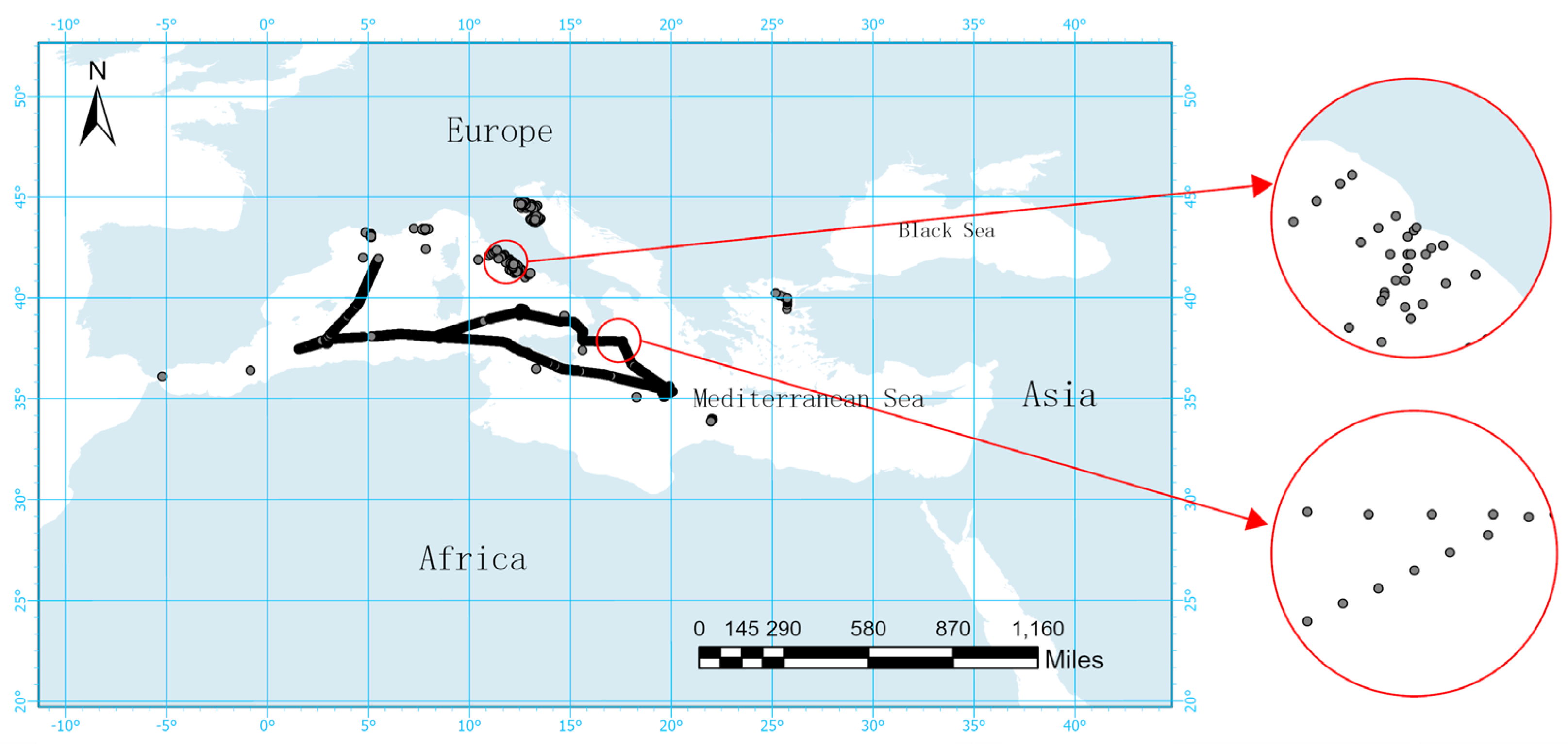
18]. The SeaWiFS and SIMBIOS project offices have established requirements for in situ data and sampling strategies to ensure the acceptability of observational results for algorithm development purposes. In situ data collected at depths less than 10 meters were selected to ensure the accuracy of the results. After screening, a total of 11,706 measurements of surface POC data from the Mediterranean were obtained. The distribution map of measurement points is depicted in
Figure 1, illustrating that the concentration of POC is higher near the coast compared to far from the coast, with relatively similar POC concentrations observed far from the coast.
2.2.2. Satellite Data
Remote sensing data and reanalysis data obtained from multiple databases, down-loaded from the Copernicus Marine Service (
https://marine.copernicus.eu/). Considering the time of collected observed POC data and the absence of corresponding satellite data in certain regions at certain times, data from May 10, 2017, to June 15, 2017, were selected for download. The products mainly include 11 bands (412nm, 443nm, 490nm, 555nm, 670nm, 547nm, 645nm, 667nm, 469nm, 488nm, 510nm) of remote sensing reflectance (Rrs), chlorophyll_a (Chl), oxygen (O2), silicate (SiO3), nitrate (NO3), phosphate (PO4), sea water salinity (SSS), euphotic zone depth (ZEU), pH, ocean mixed layer thickness (Mld), geostrophic eastward ocean velocity (Ugos), geostrophic northward ocean velocity (Vgos), sea surface temperature (SST), sea surface density (Dos), volume absorption coefficient of radiative flux in sea water due to dissolved organic matter and non-algal particles (CDM), backscattering coefficient of particles (BBP), diffuse attenuation coefficient at 490 nm (Kd_490), and suspended particulate matter (SPM) .The parameters, full name, source datasets, spatial resolution, time resolution and amount of collected remote sensing data and reanalysis data are summarized in
Table 1.
2.2.3. Matchup between In Situ and Satellite Data
This study developed a program for spatiotemporal matching between remote sensing data and measured POC data. This program averages the POC concentrations that appear in the same modeling spatial units. A total of 1532 matched data points were obtained for the period from May 15, 2017, to June 10, 2017. The data were divided into training, validation, and testing sets in a ratio of 6:2:2, respectively used for training data, parameter tuning, and testing the model's performance on the data used in this study. This approach enhances the accuracy of training and evaluating machine learning algorithms. The maximum POC concentration observed was 57.35 mg/m³, the minimum was 20.68 mg/m³, and the average was 30.59 mg/m³.
2.3. Feature Selection
In this study, GD was employed as the method for feature selection. The primary concept behind GD involves dividing the study area into different subregions based on various variables. It then compares the variances between different subregions and within each subregion to assess the explanatory power of potential variables [
19]. The GD model eliminates the linear assumption, thus the results obtained are not affected by multicollinearity among multiple variables [
20]. Spatial data discretization is crucial for identifying feature variables. Before implementing the GD model, data discretization is performed as a preliminary step [
21]. The q-value is used to represent the extent to which a variable can explain the spatial variation of the dependent variable. The formula is as follows:
In the equation, SSW stands for Within Sum of Squares, and SST stands for Total Sum of Squares. The q-value ranges from 0 to 1, where a higher q-value indicates a stronger correlation between the influencing factor and POC.
2.4. Model Selection
XGBoost is an extensible end-to-end tree boosting system. To estimate suspended particulate matter in global lakes, a XGBoost model was trained by Wen et al. [
22]. To invert global POC concentrations, a XGBoost model was also trained by Liu et al. [
23]. In this study, the selected optimal hyperparameters are as follows: the number of trees is 192, the learning rate is set to 0.1, the maximum depth per tree is 10, and the minimum weight per leaf node is 9.798.
RF was first introduced by Breiman in 2001[
24]. Today, RF widely applied in remote sensing analysis [
25], aiming to reduce overfitting and overlearning to maintain the accuracy of the results [
24]. Recent studies have shown that RF achieves higher accuracy compared to other multivariate linear regression models when considering multiple variables [
26,
27]. In this study, the parameters selected are as follows: minimum samples per leaf node is 1, maximum depth is 17, minimum samples split is 20, and the number of trees is 275.
AdaBoost is an excellent boosting algorithm that can elevate weak learning algorithms to stronger ones with higher accuracy [
28]. The parameters of the AdaBoost model used in this study are as follows: learning rate is 1 and trees are 181.
ANN is a complex network structure consisting of input layers, hidden layers, and output layers [
29]. The BPNN utilizes gradient descent to continuously adjust the net-work's weights and thresholds through backpropagation, aiming to minimize the sum of squared errors in the network. The parameters of the BPNN model used in this study are as follows: 1 input layer, 10 hidden layers, and 1 output layer. The first hidden layer consists of 89 neurons, while the remaining layers consist of 52 neurons each.
2.5. Dual Optimization of the RF Model
2.5.1. Initial Optimization of the RF Model
BO [
30,
31,
32] is a global optimization method based on sequential models. First, a probability model is constructed, defining distributions on the objective function, and then refining this model [
33]. Unlike the other two commonly used tuning methods, grid search and random search, BO utilizes previously searched points to determine the next search point and is used to solve low-dimensional black-box optimization problems. The core of the algorithm is: modeling the objective function using Gaussian process regression; constructing an acquisition function to determine the locations of the sampled points. Gaussian process predictors are widely used in Bayesian methods, requiring O(n^2) space and O(n^3) time for the operation of n datasets [
34]. Since the performance of RF is influenced by numerous hyperparameters, including the number of trees, the maximum depth of each tree, and the minimum sample number for each node, the BO algorithm was incorporated into the RF to enhance model accuracy, resulting in the BRF used in this study.
2.5.2. Re-optimization of the RF Model
Building on the BO method, TR was used to fine-tune the parameters of the BRF model, resulting in the TRRF model used in this research, which was then compared to the BRF model. The TR is based on the R packages ranger and mlrMBO. Its principle in-volves employing SMBO as the adjustment strategy [
35], the function simultaneously adjusts the randomly selected candidate variables (mtry), sample size, and node size, using out-of-bag prediction as the evaluation method, which is much more efficient than using cross-validation. The final selection of hyperparameters involves selecting the top 5% from all SMBO iterations, calculating the average value for each hyperparameter, and rounding for mtry and node size [
14]. After iterations, mtry is set to 2, min node size is set to 2, and sample fraction is set to 0.898.
2.6. Statistical Indicators Used for Model Development, Validation and Test
This study randomly divides the dataset into three parts according to the ratio of training set: validation set: test set = 6:2:2. The training set is used for model training, the validation set is used for tuning the best hyperparameters of the model, and the test set is used to evaluate the performance of the model equipped with the best hyperparameters. Bias, variance, goodness of fit (R²), root mean square error (RMSE), mean absolute percentage error (MAPE), mean absolute error (MAE) and mean squared error (MSE) are used as metrics to measure the performance of the model.
Bias is the error between the model's predicted values and the true values, describing the overall error direction of the model and characterizing the fitting ability of the learning algorithm itself. The formula is as follows:
Variance describes the dispersion of predicted values, that is, the distance between them and the expected value. The larger the variance, the more scattered the data distribution. The formula is as follows:
R² describes the degree to which the model fits the data, with 0 ≤ R² ≤ 1. If the result is 0, it indicates a poor fit of the model to the data; if the result is 1, it means the model is error-free. In general, the larger the R², the better the fit of the model. The formula for calculating R² is as follows:
RMSE describes the deviation between predicted values and actual values, and is sensitive to outliers in the data. The calculation formula is as follows:
MAPE is sensitive to relative errors and does not change with proportional changes in the target variable, making it suitable for data with large differences in the scales of the target variables. Its calculation formula is as follows:
MAE represents the average of the absolute errors between observed and predicted values. It is a linear score that treats all individual differences equally, without magnifying high differences disproportionately. Consequently, it is not sensitive to outliers. The calculation formula is as follows:
MSE represents the average of the squared differences between observed and predicted values. It is useful for measuring the average error and can evaluate the degree of variation in the data, thus indicating higher accuracy of the predictive model. The calculation formula is as follows:
To measure the model's fit, this study selected two indicators: R² and bias. To assess the predictive variability of the model across different samples, RMSE, Variance, MSE and MAE were chosen. To describe the overall error of the model, the MAPE indicator was selected.
3. Results and Discussion
3.1. Feature Selection
This study employed the GD method for factor detection and selected variable factors for model training. These factors can be categorized into three types:
The first category comprises AOPs and their mathematical combinations. AOPs are quantities sensitive to lighting conditions, including downward irradiance (Ed), upward irradiance (Eu), water-leaving radiance (LW), Rrs, radiance ratios, and their respective diffuse attenuation coefficients. These parameters are crucial for ocean remote sensing, as they are affected by the absorption and scattering of light in sea-water [
36]. Among this category, the volume attenuation coefficient of downwelling radiative flux in seawater (Kd_490) and the Rrs at wavelengths ranging from 412nm to 670nm, encompassing the red, green, and blue wavelength regions were collected. Based on the combination of Rrs values at these wavelengths, various spectral indices and ratios were computed, including band ratios (e.g., red/green, red/blue, blue/green), CI, normalized difference carbon index (NDCI), band ratio difference index (BRDI), MNDCI, and maximum band ratio (MBR)[
8].
The second category encompasses features potentially associated with POC. This study includes Chl, O2, SiO3, NO3, PO4, SSS, Euphotic zone depth (EP), pH, Mld, Ugos, Vgos, SST, and DOS [
37]. Chlorophyll_a concentration serves as an indicator of photosynthesis intensity and phytoplankton biomass in the ocean. Oxygen concentration influences microbial respiration, thereby impacting the remineralization process of POC and subsequently affecting its concentration in the ocean surface. In oxygen-depleted zones, a considerable portion of POC generated through surface ocean photosynthesis may sink into the deep sea, further influencing surface POC concentration [
38]. Silicates significantly influence the production of particulate carbon by phytoplankton [
39]. The concentration of POC greatly influences the content of bioavailable phosphorus in the ocean surface, because of POC serves as a carrier of endogenous phosphorus [
40]. Sea surface salinity and temperature exert direct or indirect effects on the growth and reproduction of marine surface flora and fauna. EP is closely linked to the photosynthesis of surface marine plants. PH significantly influences various chemical processes by creating different chemical environments. Changes in MLD result in variations in the distribution of various nutrient salts. Dissolved oxygen distribution, including variations due to light penetration, also impacts the concentration of POC in the surface ocean.
The third category comprises IOPs, which are solely influenced by the composition of the water and remain constant regardless of changes in light conditions. IOPs encompass various components such as absorption and attenuation coefficients within the water. In this study, the backscattering coefficient of particles is selected as a candidate feature from the IOPs. These parameters serve as candidate features for the model established in this study.
Following the determination of the range of study features, this research employed the R language software package developed by Song et al. for geographical detection [
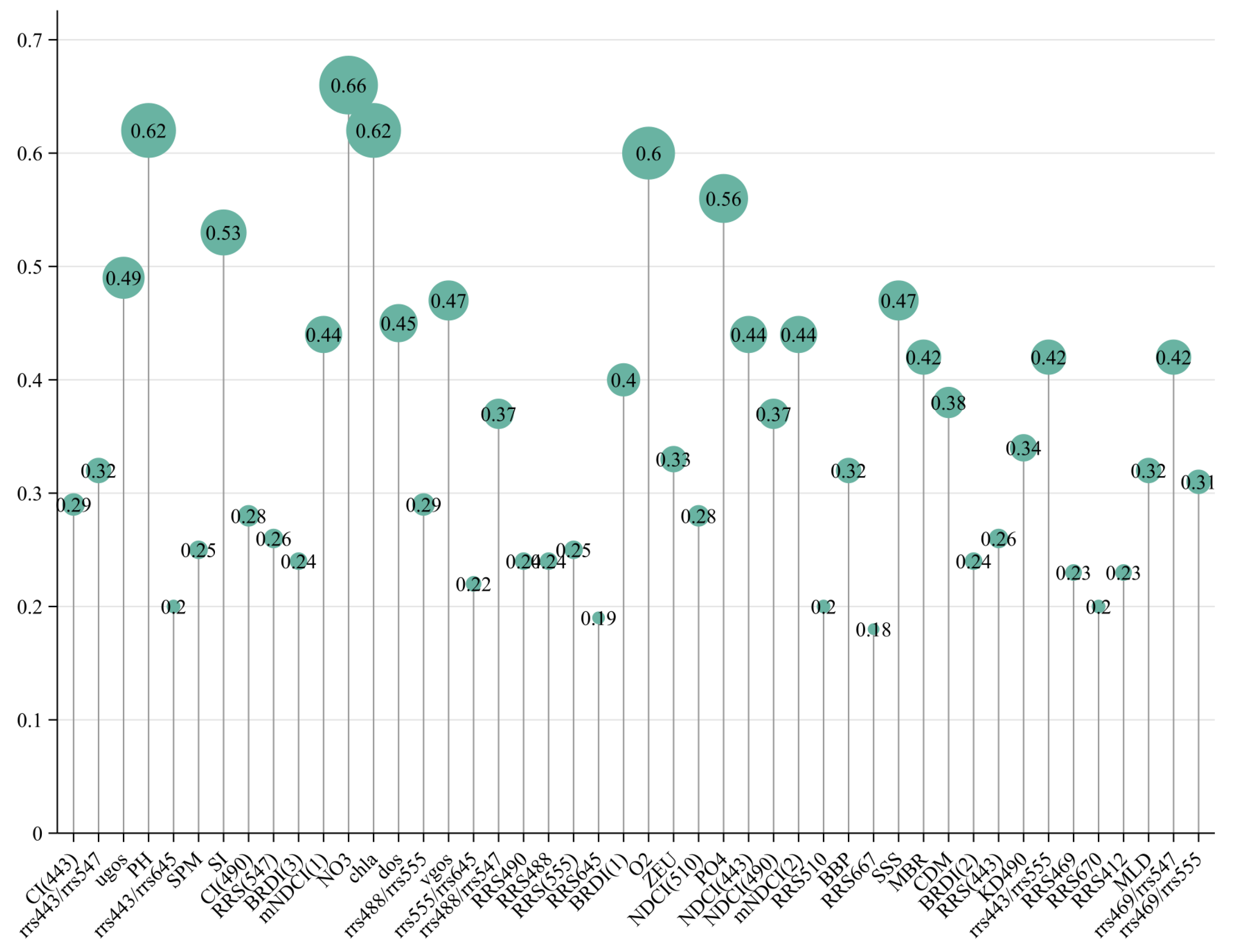
19], before employing this method, it is necessary to discretize continuous variables. The GD package offers four discretization methods: equal intervals, geometric intervals, quantiles, and natural breaks. The factor detection results are depicted in
Figure 2. The interaction detection results suggest either enhanced bivariate or non-linear enhancement, both of which are selected. In the factor detection results, variables with q < 0.45 are regarded as weakly correlated with surface POC, whereas those with q > 0.45 are deemed strongly correlated. Finally, ten variables were selected to train the model used to estimate the sea surface POC, include MNDCI(I), NDCI (443), and Kd_490 from AOPs and their mathematical combinations, BBP from IOPs, and other features related to POC such as NO3, O2, PO4, SPM, SSS, and Chl. The selection was based on excluding factors from those with higher q-values that are not mechanistically related to POC. Oxygen concentration affects microbial respiration, which in turn influences the remineralization of POC, thus affecting the surface POC concentration in the ocean. POC can increase the rate of nitrogen mineralization and also affect denitrification and nitrate retention rates in the ocean [
38], it also serves as a carrier of endogenous phosphorus, and its concentration significantly impacts the availability of phosphorus to surface marine organisms [
40]. Chlorophyll concentration reflects the intensity of photosynthesis and the biomass of oceanic plants. Sea surface salinity directly or indirectly influences the growth and reproduction of marine organ-isms. Suspended particulate organic matter serves as a crucial carbon source in the ocean, contributing to the increase of POC. All these factors play a significant role in the formation and transformation of POC.
3.2. Machine Learning Model for POC
3.2.1. Accuracy of the Model on Different Datasets
The BO method was employed to adjust hyperparameters for the RF and XGBoost models, whereas parameters for the AdaBoost and BPNN models were manually set.
The BRF, XGBoost, AdaBoost, and BPNN models demonstrate strong fitting capabilities for nonlinear functions and excel in completing multivariate regression tasks. To enhance the models' generalization ability, this study transformed the target variable, surface POC in the ocean, by taking the base 10 logarithm as the model input.
Table 2 presents the evaluation metrics of the four machine learning models on the training, validation, and test sets, where the metrics highlighted in bold represent the best performance of each model on the corresponding dataset. Among the four models, the BRF model exhibits the best performance, with a bias of -0.001, variance of 0.004, R² of 0.85, RMSE of 0.026 log(mg/m³), and MAPE of 1.284% on the test set. Therefore, when estimating the concentration of surface POC in the Mediterranean Sea, the BRF model exhibits strong superiority in both generalization ability and fitting degree. The partitioning of water bodies based on the contribution of organic particles to suspended particles shows that the surface water in the Mediterranean Sea is predominantly organic in nature. Previous studies have similarly highlighted the significant advantages of the RF algorithm over other machine learning algorithms in estimating the concentration of POC in organic water [
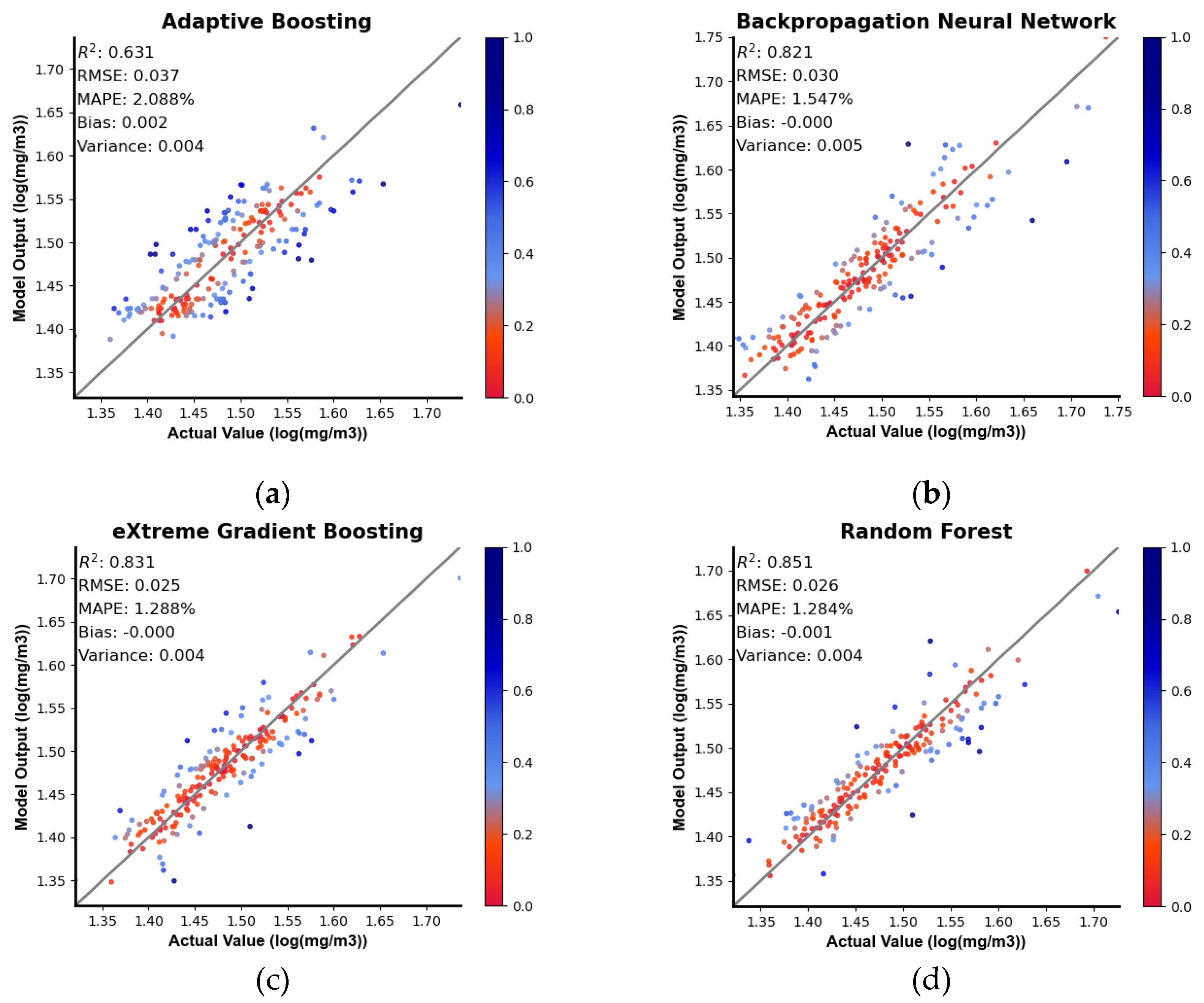
41], this also elucidates why the BRF algorithm outperforms others in estimating the concentration of surface POC in the Mediterranean Sea. We utilize Normalized Residuals to detect model outliers and assess the fitting degree of the models. In this study, we plot scatter plots of the normalized residuals of the predictions from the four models on the test set, as shown in
Figure 3, where the color of the points reflects the magnitude of the normalized residuals. From the scatter plot, it is more visually apparent that the AdaBoost algorithm has poorer fitting compared to the other three algorithms, while the RF algorithm exhibits the best fitting with an R² of 0.851. The measured data values in our study are relatively concentrated, mostly ranging from 20 to 40 mg/m³. This suggests that for predicting low concentrations of POC, BRF, XGBoost, and BPNN models are all suitable, with the BRF model performing the best.
3.2.2. Re-optimization of the RF Model
To further optimize the model for higher accuracy, this study employed TR developed by Probst et al., specifically designed for parameter tuning of RF. SMBO was utilized as the tuning strategy, with out-of-bag prediction used for evaluation [
19]. The evaluation metrics utilized include R², MAE and MSE. A comparison is made between the precision of adjusting the hyperparameters of RF using TR and Python's BO method. The results are presented in
Table 3.
In
Table 3, it is observed that the TRRF model outperforms the BRF model in terms of R², MSE, and MAE metrics. Besides achieving higher accuracy, TRRF utilizes out-of-bag prediction as the evaluation method during parameter tuning, which is notably faster compared to using cross-validation or splitting the dataset for evaluation [
14], achieving improvement in both accuracy and speed.
3.3. Assessment of the TRRF Model
3.3.1. Comparison of TRRF Products and NASA Products
Comparison was made between the Mediterranean POC estimation products obtained from the TRRF and the POC products retrieved using NASA's band ratio algorithm for May and June 2017. POC products for May and June 2017 were downloaded from NASA OCEAN COLOR, and the deviations as well as percentage deviations between the products derived from the two algorithms were calculated.
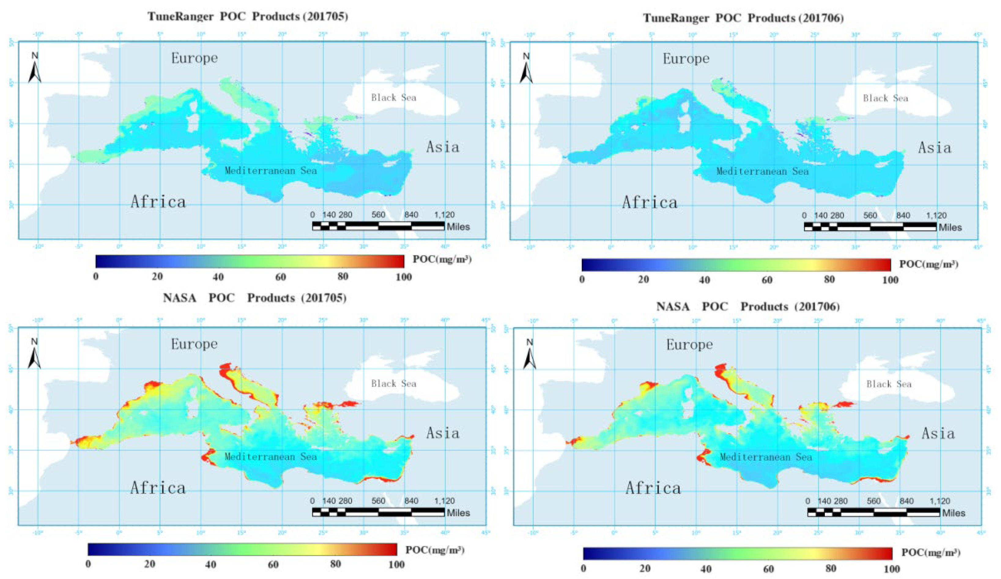
The comparison illustrated by
Figure 4 reveals that the algorithm employed by NASA and the TRRF model in this study exhibit similar spatial distributions of POC. POC demonstrates a pattern of higher concentrations in the north and lower concentrations in the south, higher levels in the west and lower levels in the east, and elevated concentrations near the coast compared to far from the coast. Given the geographical positioning of the Mediterranean, it is apparent that Europe, situated to its west and north, experiences greater economic development in comparison to Africa to its south and Asia to its east. Rapid economic development can contribute to heightened environmental pollution, leading to elevated levels of nitrogen, phosphorus, and other nutrients in the water, which may result in phenomena such as algal blooms. Elements such as nitrogen and phosphorus are closely associated with particulate organic matter (POM) [
42]. An increase in the content of nutrients such as nitrogen and phosphorus lead to a rise in POM content. As POC is a significant component of POM, the increase in nutrients results in an elevation of POC content. This phenomenon explains the distribution pattern where POC concentrations are higher in the northern and western parts of the Mediterranean compared to the southern and eastern parts. Many nutrients accumulate near the coast, with some diffusing further, thus resulting in higher POC concentrations near the coast than far from the coast. Over 80% of POC concentrations fall within the range of 0-50 mg/m³, with only a portion estimated by NASA exceeding 50 mg/m³ in coastal areas. Overall, the POC concentrations estimated using TRRF model are lower than those estimated by NASA for the Mediterranean.
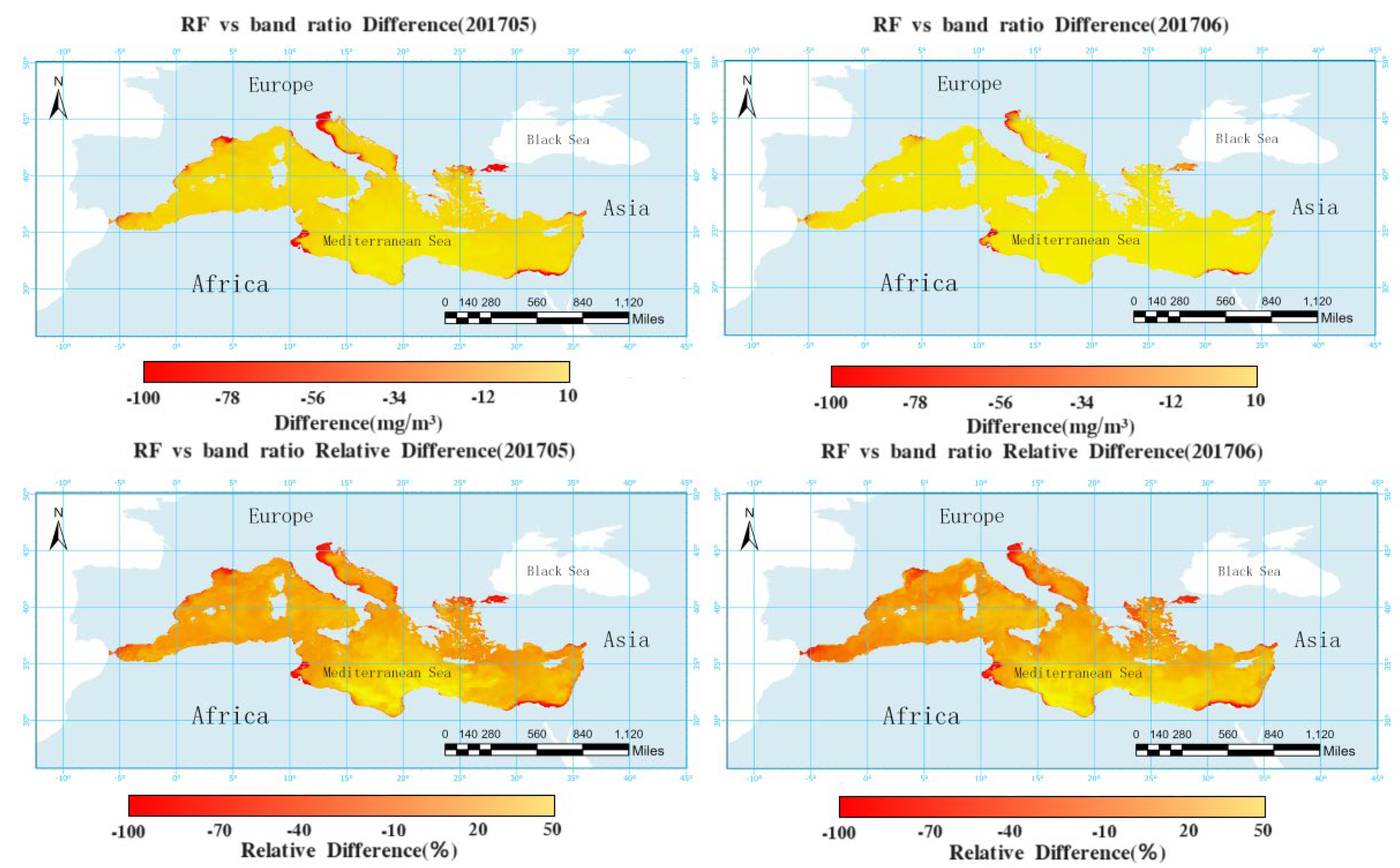
Figure 5 depicts the deviations and percentage deviations of the Mediterranean POC products estimated by TRRF and the band ratio algorithm employed in NASA products for May and June 2017. In May 2017, the deviation between the two products was less than 10 mg/m³, accounting for 82.29% of the data, and less than 20 mg/m³, accounting for 96.16% of the data, with only a few coastal areas exhibiting deviations greater than 20 mg/m³. Comparing the percentage deviations of the two products, it was found that 81.80% of the areas had a percentage deviation of less than 20%, 92.25% had a percentage deviation of less than 30%, and 98.03% had a percentage deviation of less than 50%. In June 2017, the deviation of the two products was less than 10 mg/m³, accounting for 87.11%, and less than 20 mg/m³, accounting for 96.47%, with a small number of coastal areas having deviations greater than 20 mg/m³. The percentage deviation of less than 20% was 76.66%, less than 30% was 93.16%, and less than 50% was 98.05%. In terms of dynamic time, the deviation in May 2017 was slightly larger than that in June 2017, while the percentage deviation was almost the same. Generally, there are no significant changes in the marine environment of the Mediterranean Sea within two consecutive months, so it is reasonable that the deviations and percentage deviations obtained by the two algorithms are almost consistent over two months. From a spatial perspective, the distribution of POC not only demonstrates characteristics of higher concentrations in the north, lower concentrations in the south, elevated levels in the west, lower levels in the east, and higher concentrations near the coast compared to far from the coast, but also the deviations and percentage deviations of the products exhibit similar patterns. This is attributed to the fact that both the TRRF and the band ratio algorithm show less accuracy in estimating POC in complex marine environments compared to simpler environments. When estimating POC in environments with high nutrient content and intense human activities, significant errors may occur, which do not follow a specific pattern. Therefore, the deviations and percentage deviations of the two products may become relatively large due to the accumulation of errors.
3.3.2. Comparison between TRRF Products, NASA Products, and Actual Measured Values
From
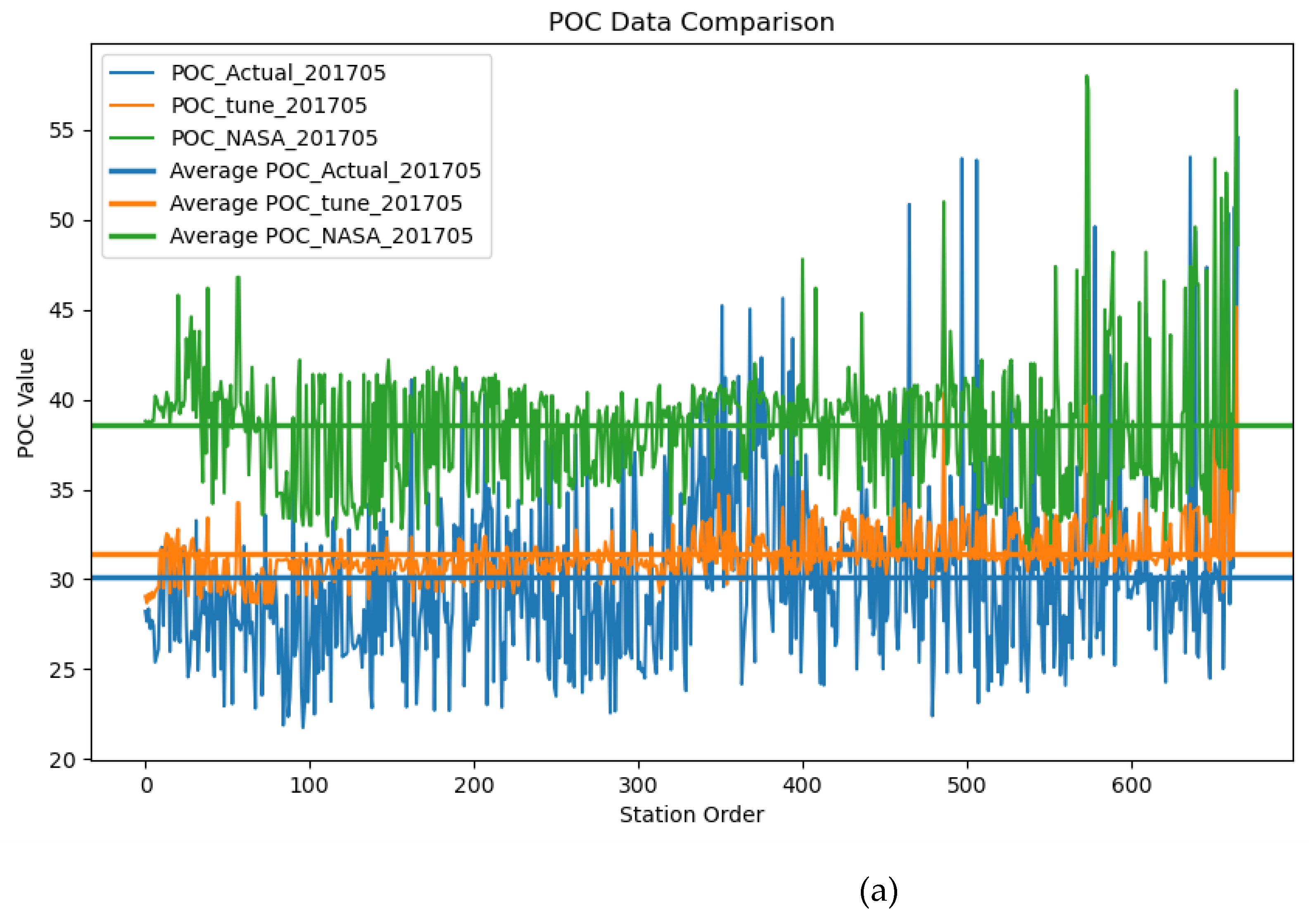
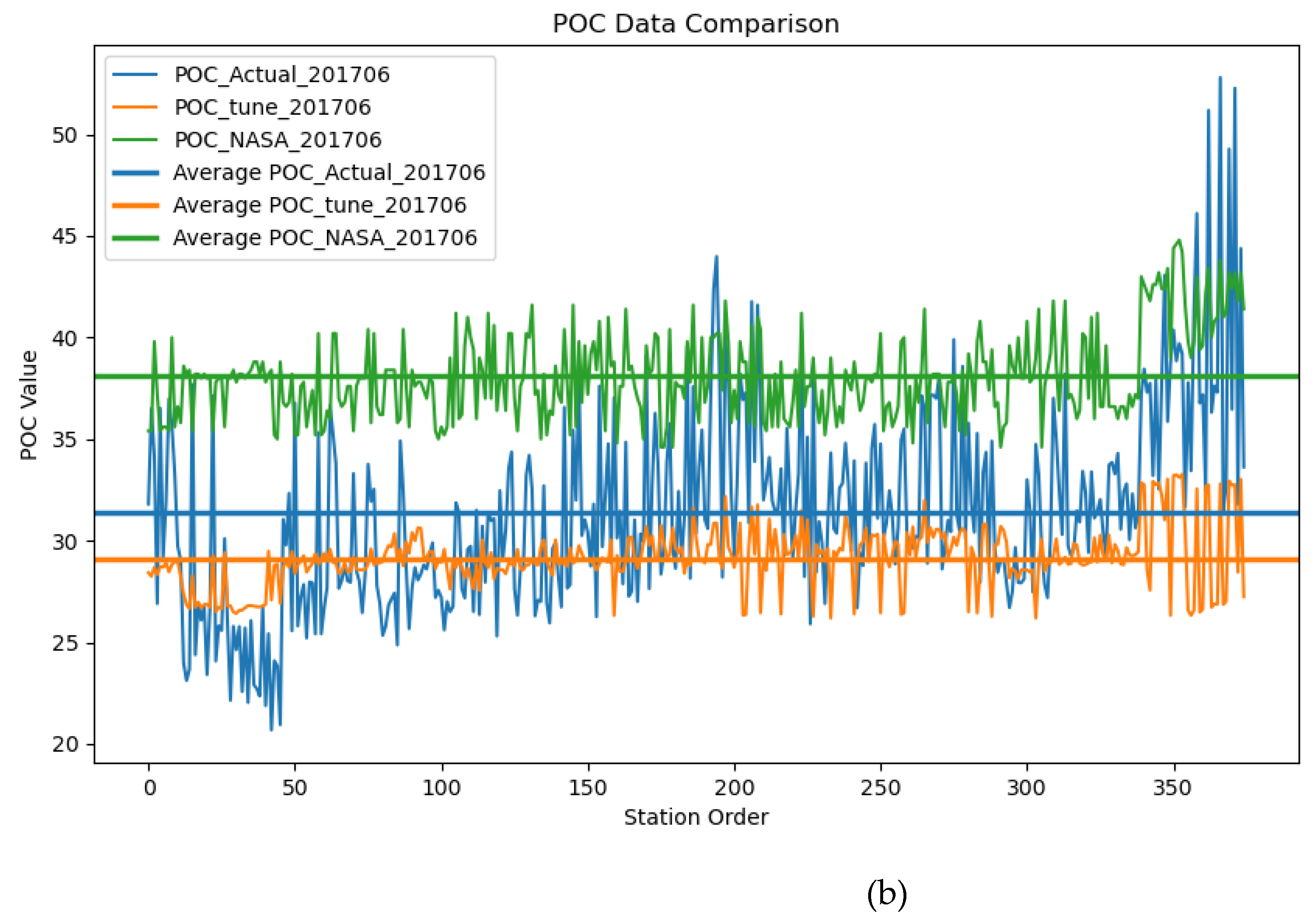
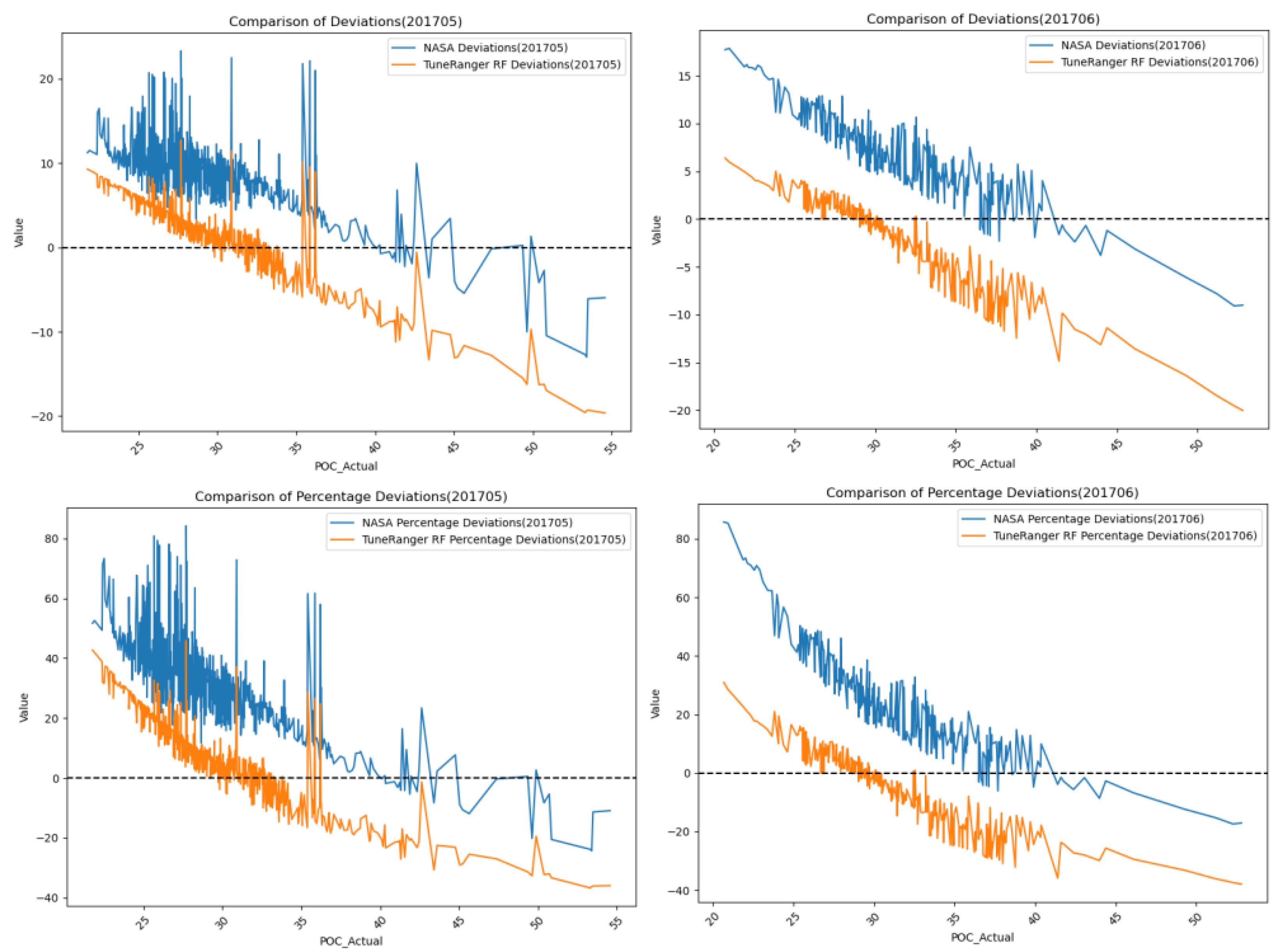
Figure 6, the lines represent the POC values at different measurement stations, while the horizontal lines represent the average values of the measured values and the two products. It can be observed that the POC values obtained by the TRRF are closer to the measured values in May and June 2017, while the NASA products tend to overestimate the surface POC concentration in the Mediterranean Sea to a greater extent. This also indicates that the products obtained in this study are more suitable for estimating the surface POC in the Mediterranean Sea, providing assistance in studying the dynamics of POC in the Mediterranean. From each line, the curve corresponding to the TRRF product is relatively smooth, with POC concentrations mostly concentrated near the average value, while the curve corresponding to the NASA product using the band ratio algorithm is more erratic, with larger variations in POC concentration. This may be because the band ratio algorithm is more sensitive to sensor noise and atmospheric uncertainties, and less capable of fitting nonlinear relationships than machine learning algorithms. It is more sensitive to changes in influencing factors, resulting in greater fluctuations in the estimated POC concentration. To further compare the differences between the products obtained by the two algorithms and the measured values, this study presents the deviations and percentage deviations between the TRRF products, NASA products, and the measured values for May and June 2017, as shown in
Figure 7.
Figure 7 is a line plot with the measured POC values on the x-axis. It is evident from the graph that, at lower POC levels, both algorithms tend to overestimate the POC values to some extent, while at higher POC levels, they tend to underestimate the POC values. What was not previously observed is that, at lower POC values, the deviation of the TRRF from the measured values is smaller than that of NASA's band ratio algorithm. However, after POC exceeds approximately 40 mg/m³, the deviation of the TRRF algorithm from the measured values becomes larger than that of NASA's band ratio algorithm. The reason may be that the POC data collected in this study are mostly concentrated in the range of 20-40 mg/m³, hence the advantage in estimating POC within this concentration range. In the Mediterranean Sea, POC concentrations higher than 40 mg/m³ are mostly concentrated in coastal areas, where data collection is relatively limited.
3.3.3. The Impact of Human Activities on the Distribution of Surface POC In the Medi-terranean Sea
As depicted in
Figure 4, the surface POC concentration in the Mediterranean Sea exhibits characteristics of being higher in the west, lower in the east, higher in the north, lower in the south, higher near the coast, and lower far from the coast. There was a finding that nutrient levels influence microbial activities, thereby affecting POC concentration. Utilized was stable isotope analysis, revealing that 20% of the POM in the North South China Seas comes from terrestrial inputs [
43], with POC being a component of POM and thus also influenced by terrestrial inputs. Indicated by research is that human activities in the Yangtze River Basin can significantly alter the coastal carbon cycle, thereby affecting the concentration of POC [
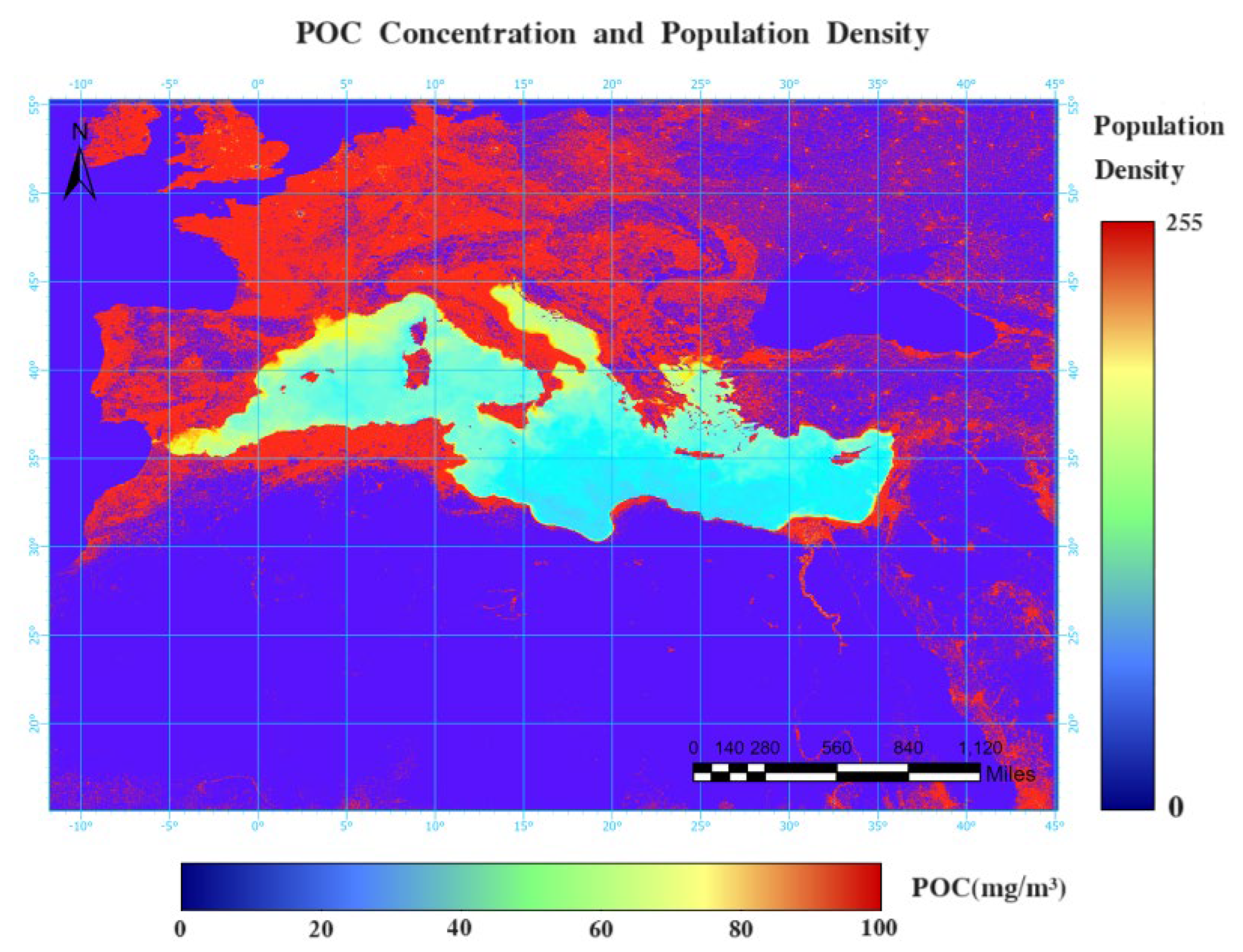
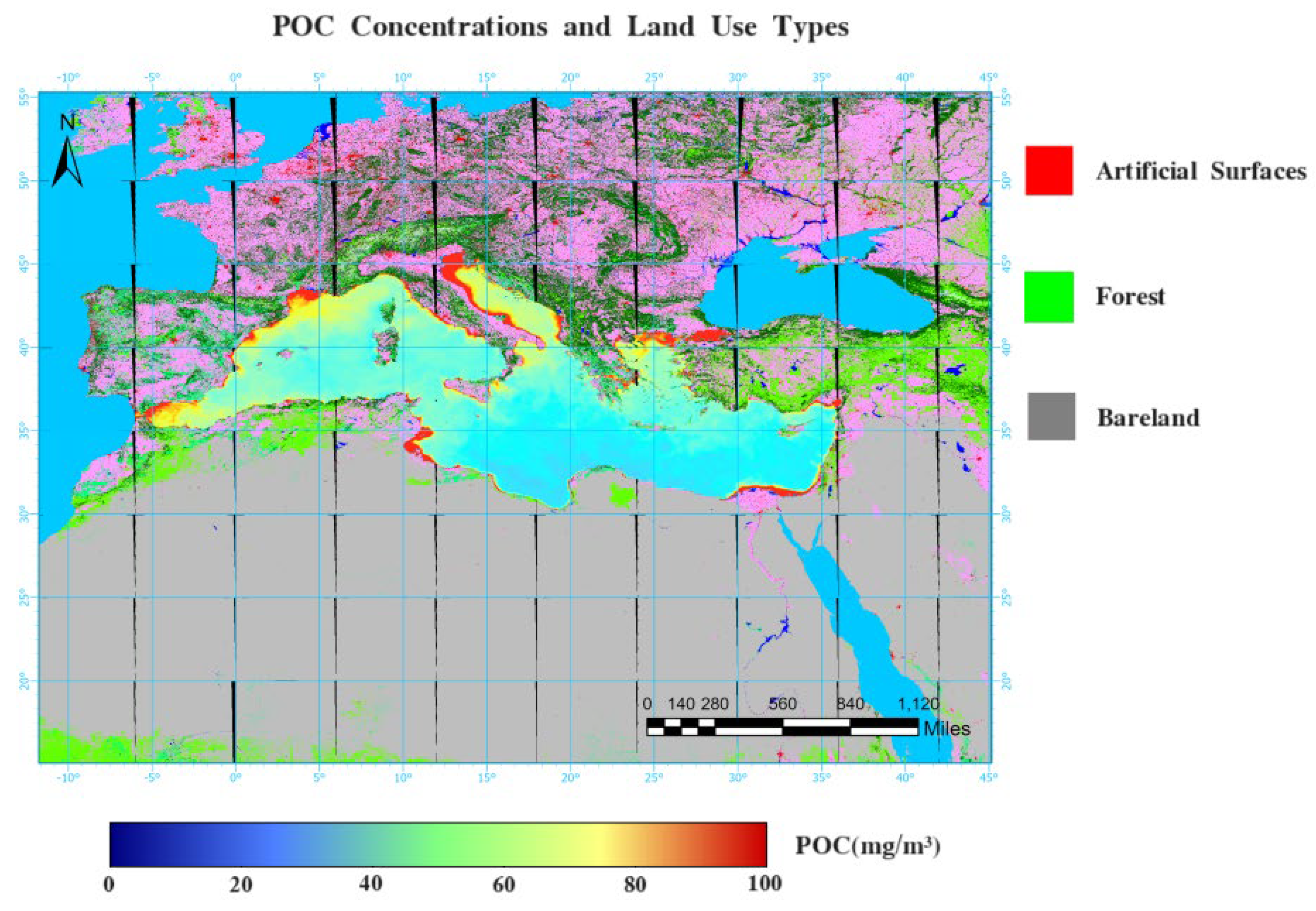
44]. Therefore, regarding the distribution of POC concentration in the Mediterranean Sea, the higher concentration near the coast and lower concentration far from the coast can be attributed to the significant influence of human activities in coastal areas, leading to increased terrestrial inputs of POC. The characteristics of higher concentration in the west, lower in the east, higher in the north, and lower in the south can be analyzed based on population density, GDP, and land use types of coastal cities in the Mediterranean.
From
Figure 8 and
Figure 9, it can be observed that in the north-south direction, the northern regions of the Mediterranean have higher population densities, including countries such as Spain, France, Milan, Rome, Greece, etc. The land use types in these regions are mostly artificially modified land, with some forested areas where vegetation covers more than 30% of the land. These countries also have relatively high GDPs. In contrast, the southern regions have lower population densities, including countries such as Egypt, Libya, Tunisia, Morocco, etc. The land use types in these regions are mostly barren lands or even deserts with vegetation covering less than 10% of the land. The GDP of cities in the south is lower than that in the north. Coastal areas are typically defined as regions within 40 miles of the coastline. For the Mediterranean, due to the specific natural resources and economic activities in coastal areas, the population density along the Mediterranean coast is more than twice that of the entire Mediterranean region. In recent years, the tourism industry has rapidly developed along the northern coast of the Mediterranean. Currently, over 25% of the world's hotels are located in the Mediterranean region. However, this development has also put significant environmental pressure on the Mediterranean [
45]. While GDP continues to rise, commercial fishing and tourism industries are rapidly developing. The use of artisanal fishing and exploitation of red coral have significantly impacted the biodiversity of the Mediterranean region. The increase in recreational activities also affects both species and habitats. The arrival of nearly 120 million tourists each year further burdens the Mediterranean environment [
46]. All these factors contribute to intensified eutrophication and influence microbial activities, resulting in an increase in surface POC concentration along the coastal areas of the Mediterranean, displaying the characteristic of higher near the coast, lower far from the coast. Population density, GDP, and land use types are robust indicators reflecting human activities. Therefore, by observing
Figure 8 and
Figure 9, it is evident that cities in the western and northern regions of the Mediterranean have higher population densities, higher GDPs, and greater degrees of anthropogenic land development. This explains why the surface POC concentration in the Mediterranean exhibits the pattern of being higher in the west and lower in the east, and higher in the north and lower in the south.
4. Discussion
To estimate the surface POC in the Mediterranean, we selected relationships be-tween apparent optical parameters, inherent optical parameters, water components, and POC concentrations. Algorithms were chosen through feature selection using GD, considering three categories of 47 factors likely to affect POC concentration. Ten factors most suitable for estimating Mediterranean POC concentration were identified. The dataset was split into training, validation, and test sets in a 6:2:2 ratio. Models were trained using the BRF algorithm, Bayesian optimized XGBoost algorithm, AdaBoost algorithm, and BPNN algorithm. Among the four algorithms, the BRF algorithm performed the best, with a deviation of -0.001, a variance of 0.004, R² of 0.851, RMSE of 0.025 log10(mg/m³), and MAPE of 1.268%, achieving high accuracy. To further enhance the BRF algorithm's performance in estimating surface POC in the Mediterranean, we utilized parameter tuning using the TR, which resulted in the TRRF model used in this research. Compared to BRF, TRRF yielded higher accuracy and faster speed. Evaluation metrics for the BRF model using Python were R² of 0.851, MSE of 1.125 (mg/m³) ², and MAE of 1.045 (mg/m³). With parameter tuning using the TR, evaluation metrics for the TRRF model improved significantly to an R² of 0.868, MSE of 1.119 (mg/m³) ², and MAE of 1.040 (mg/m³). Subsequently, the TRRF model was used for inversion. The resulting product was compared with NASA standard products, and it was found that both the deviation and percentage deviation were small. Furthermore, a comparison was made between the TRRF products, NASA products, and actual measurements, considering factors such as true values, averages, deviations, and percentage deviations. It was concluded that the TRRF products outperformed NASA products in estimating POC in the Mediterranean, providing significant assistance for studying the dynamics of POC in the Mediterranean. Finally, using the TRRF, surface POC products for May 2017 and June 2017 were produced, revealing spatial distribution characteristics of POC: higher near the coast and lower far from the coast, higher in the west and lower in the east, and higher in the north and lower in the south. The study also discussed the impact of human activities on surface POC concentration in the Mediterranean, indicating that intense human activities can significantly increase POC concentration.
However, this study still has some shortcomings that need improvement:
The collected Mediterranean observational data in this study are mostly concen-trated in the range of 20-40 mg/m³, lacking a sufficient number of samples with high POC concentrations. This results in the algorithm performing well at lower POC concentrations but poorly in estimating POC concentrations higher than 40 mg/m³. Therefore, in the future, more surface POC samples from the Mediterranean should be collected to increase the proportion of high-concentration POC samples and improve the accuracy of the model.
When exploring the impact of human activities on the spatial distribution of POC in the Mediterranean, this study qualitatively described the distribution based on maps rather than quantitatively. In the future, methods will be considered to quantitatively assess the influence of human activities on POC distribution.
Author Contributions
Conceptualization, C.L.; methodology, C.L. and H.W.; software, L.C. and Z.M.; validation, H.W., L.C., and L.W.; formal analysis, C.L. and Z.M.; investigation, C.Y.; resources, C.Y.; data curation, C.L.; writing—original draft preparation, C.L.; writing—review and editing, H.W.; visualization, C.L. and L.C.; supervision, L.C. and H.W.; project administration, H.W.; funding acquisition, C.L. All authors have read and agreed to the published version of the manuscript.
Funding
This research received no external funding.
Institutional Review Board Statement
Not applicable.
Informed Consent Statement
Not applicable.
Data Availability Statement
Not applicable.
Acknowledgments
The authors would like to thank the Assistant Editor of this article and anonymous reviewers for their valuable suggestions and comments.
Conflicts of Interest
The authors declare no conflicts of interest.
References
- Kharbush, J.J.; Close, H.G.; Van Mooy, B.A.; Arnosti, C.; Smittenberg, R.H.; Le Moigne, F.A.; Mollenhauer, G.; Scholz-Böttcher, B.; Obreht, I.; Koch, B.P. Particulate organic carbon deconstructed: Molecular and chemical com-position of particulate organic carbon in the ocean. Front Mar Sci 2020, 7, 518. [Google Scholar] [CrossRef]
- Brewin, R.J.; Sathyendranath, S.; Platt, T.; Bouman, H.; Ciavatta, S.; Dall'Olmo, G.; Dingle, J.; Groom, S.; Jönsson, B.; Kostadinov, T.S. Sensing the ocean biological carbon pump from space: A review of capabilities, concepts, research gaps and future developments. Earth-Sci Rev 2021, 217, 103604. [Google Scholar] [CrossRef]
- Stramski, D.; Reynolds, R.A.; Kahru, M.; Mitchell, B.G. Estimation of particulate organic carbon in the ocean from satellite remote sensing. Science 1999, 285, 239–242. [Google Scholar] [CrossRef] [PubMed]
- Woźniak, S.B.; Darecki, M.; Zabłocka, M.; Burska, D.; Dera, J. New simple statistical formulas for estimating surface concentrations of suspended particulate matter (SPM) and particulate organic carbon (POC) from remote-sensing re-flectance in the southern Baltic Sea. Oceanologia 2016, 58, 161–175. [Google Scholar] [CrossRef]
- Son, Y.B.; Gardner, W.D.; Mishonov, A.V.; Richardson, M.J. Multispectral remote-sensing algorithms for particulate organic carbon (POC): The Gulf of Mexico. Remote Sens Environ 2009, 113, 50–61. [Google Scholar] [CrossRef]
- Stramski, D.; Reynolds, R.A.; Babin, M.; Kaczmarek, S.; Lewis, M.R.; Röttgers, R.; Sciandra, A.; Stramska, M.; Twardowski, M.S.; Franz, B.A. Relationships between the surface concentration of particulate organic carbon and optical properties in the eastern South Pacific and eastern Atlantic Oceans. Biogeosciences 2008, 5, 171–201. [Google Scholar] [CrossRef]
- Le, C.; Lehrter, J.C.; Hu, C.; MacIntyre, H.; Beck, M.W. Satellite observation of particulate organic carbon dynamics on the L ouisiana continental shelf. J. Geophys. Res. Ocean. 2017, 122, 555–569. [Google Scholar] [CrossRef] [PubMed]
- Stramski, D.; Joshi, I.; Reynolds, R.A. Ocean color algorithms to estimate the concentration of particulate organic carbon in surface waters of the global ocean in support of a long-term data record from multiple satellite missions. Remote Sens Environ 2022, 269, 112776. [Google Scholar] [CrossRef]
- Cai, S.; Wu, M.; Le, C. Satellite Observation of the Long-Term Dynamics of Particulate Organic Carbon in the East China Sea Based on a Hybrid Algorithm. Remote Sens. 2022, 14, 3220. [Google Scholar] [CrossRef]
- Sauzède, R.; Johnson, J.E.; Claustre, H.; Camps-Valls, G.; Ruescas, A.B. Estimation of oceanic particulate organic carbon with machine learning. Isprs Annals of the Photogrammetry, Remote Sensing and Spatial Information Sciences 2020, 2, 949–956. [Google Scholar] [CrossRef]
- Fellous, S.; Bendjama, A.; Benzaoui, Y. Use Of Machine Learning Algorithms And In Situ Data For Estimating Par-ticulate Organic Carbon From The Mediterranean Sea. Larhyss Journal P-Issn 1112-3680/E-Issn 2521-9782 2023, (56), 179–192.
- Wu, J.; Chen, X.; Zhang, H.; Xiong, L.; Lei, H.; Deng, S. Hyperparameter optimization for machine learning models based on Bayesian optimization. J. Electron. Sci. Technol. 2019, 17, 26–40. [Google Scholar] [CrossRef]
- Alibrahim, H.; Ludwig, S.A. In Hyperparameter optimization: Comparing genetic algorithm against grid search and bayesian optimization, 2021 IEEE Congress on Evolutionary Computation (CEC), 2021; IEEE: 2021; pp. 1551–1559.
- Probst, P.; Wright, M.N.; Boulesteix, A.L. Hyperparameters and tuning strategies for random forest. Wiley Interdisci-plinary Reviews: Data Mining and Knowledge Discovery 2019, 9, e1301. [Google Scholar] [CrossRef]
- Wang, J.; Zhang, T.; Fu, B. A measure of spatial stratified heterogeneity. Ecol Indic 2016, 67, 250–256. [Google Scholar] [CrossRef]
- Tanhua, T.; Hainbucher, D.; Schroeder, K.; Cardin, V.; Álvarez, M.; Civitarese, G. The Mediterranean Sea system: A review and an introduction to the special issue. Ocean Sci 2013, 9, 789–803. [Google Scholar] [CrossRef]
- Stramska, M.; Stramski, D. Variability of particulate organic carbon concentration in the north polar Atlantic based on ocean color observations with Sea-viewing Wide Field-of-view Sensor (SeaWiFS). Journal of Geophysical Re-search: Oceans 2005, 110. [Google Scholar] [CrossRef]
- Werdell, P.J.; Fargion, G.S.; McClain, C.R.; Bailey, S.W. The SeaWiFS bio-optical archive and storage system (Sea-BASS): Current architecture and implementation, 2002.
- Song, Y.; Wang, J.; Ge, Y.; Xu, C. An optimal parameters-based geographical detector model enhances geographic characteristics of explanatory variables for spatial heterogeneity analysis: Cases with different types of spatial data. Gisci Remote Sens 2020, 57, 593–610. [Google Scholar] [CrossRef]
- Wang, X.; Meng, Q.; Zhang, L.; Hu, D. Evaluation of urban green space in terms of thermal environmental benefits using geographical detector analysis. Int J Appl Earth Obs 2021, 105, 102610. [Google Scholar] [CrossRef]
- Zhang, Z.; Song, Y.; Wu, P. Robust geographical detector. Int J Appl Earth Obs 2022, 109, 102782. [Google Scholar] [CrossRef]
- Wen, Z.; Wang, Q.; Ma, Y.; Jacinthe, P.A.; Liu, G.; Li, S.; Shang, Y.; Tao, H.; Fang, C.; Lyu, L. Remote estimates of suspended particulate matter in global lakes using machine learning models. Int Soil Water Conse 2024, 12, 200–216. [Google Scholar] [CrossRef]
- Liu, H.; Li, Q.; Bai, Y.; Yang, C.; Wang, J.; Zhou, Q.; Hu, S.; Shi, T.; Liao, X.; Wu, G. Improving satellite retrieval of oceanic particulate organic carbon concentrations using machine learning methods. Remote Sens Environ 2021, 256, 112316. [Google Scholar] [CrossRef]
- Breiman, L. Random forests. Mach Learn 2001, 45, 5–32. [Google Scholar] [CrossRef]
- Belgiu, M.; Drăguţ, L. Random forest in remote sensing: A review of applications and future directions. Isprs J Pho-togramm 2016, 114, 24–31. [Google Scholar] [CrossRef]
- Hultquist, C.; Chen, G.; Zhao, K. A comparison of Gaussian process regression, random forests and support vector regression for burn severity assessment in diseased forests. Remote Sens Lett 2014, 5, 723–732. [Google Scholar] [CrossRef]
- Wang, S.; Jin, X.; Adhikari, K.; Li, W.; Yu, M.; Bian, Z.; Wang, Q. Mapping total soil nitrogen from a site in north-eastern China. Catena 2018, 166, 134–146. [Google Scholar] [CrossRef]
- Ying, C.; Qi-Guang, M.; Jia-Chen, L.; Lin, G. Advance and prospects of AdaBoost algorithm. Acta Automatica Sinica 2013, 39, 745–758. [Google Scholar] [CrossRef]
- McCulloch, W.S.; Pitts, W. A logical calculus of the ideas immanent in nervous activity. The Bulletin of Mathemati-cal Biophysics 1943, 5, 115–133. [Google Scholar] [CrossRef]
- Brochu, E.; Cora, V.M.; De Freitas, N. A tutorial on Bayesian optimization of expensive cost functions, with application to active user modeling and hierarchical reinforcement learning. Arxiv Preprint Arxiv:1012.2599 2010.
- Snoek, J.; Larochelle, H.; Adams, R.P. Practical bayesian optimization of machine learning algorithms. Adv. Neural Inf. Process. Syst. 2012, 25. [Google Scholar]
- Mockus, J.; Mockus, J. The Bayesian approach to local optimization; Springer: 1989.
- Wang, X.; Jin, Y.; Schmitt, S.; Olhofer, M. Recent advances in Bayesian optimization. Acm Comput Surv 2023, 55, 1–36. [Google Scholar] [CrossRef]
- Chalupka, K.; Williams, C.K.; Murray, I. A Framework for Evaluating Approximation Methods for Gaussian Process Regression. J Mach Learn Res 2013, 14. [Google Scholar]
- Jones, D.R.; Schonlau, M.; Welch, W.J. Efficient global optimization of expensive black-box functions. J Global Optim 1998, 13, 455–492. [Google Scholar] [CrossRef]
- Zaneveld, J.R.V. Light and water: Radiative transfer in natural waters. In JSTOR: 1995.
- Cavan, E.L.; Trimmer, M.; Shelley, F.; Sanders, R. Remineralization of particulate organic carbon in an ocean oxygen minimum zone. Nat Commun 2017, 8, 14847. [Google Scholar] [CrossRef]
- Stelzer, R.S.; Thad Scott, J.; Bartsch, L.A.; Parr, T.B. Particulate organic matter quality influences nitrate retention and denitrification in stream sediments: Evidence from a carbon burial experiment. Biogeochemistry 2014, 119, 387–402. [Google Scholar] [CrossRef]
- Egge, J.K.; Jacobsen, A. Influence of silicate on particulate carbon production in phytoplankton. Mar Ecol Prog Ser 1997, 147, 219–230. [Google Scholar] [CrossRef]
- Guo, M.; Li, X.; Wang, Y.; Zhang, Y.; Fu, Q.; Huguet, A.; Liu, G. New insights into the mechanism of phosphate re-lease during particulate organic matter photodegradation based on optical and molecular signatures. Water Res 2023, 236, 119954. [Google Scholar] [CrossRef]
- Wu, H.; Cui, L.; Wang, L.; Sun, R.; Zheng, Z. A method for estimating particulate organic carbon at the sea surface based on geodetector and machine learning. Front Mar Sci 2023. [Google Scholar] [CrossRef]
- Schneider, B.; Schlitzer, R.; Fischer, G.; Nöthig, E.M. Depth-dependent elemental compositions of particulate organ-ic matter (POM) in the ocean. Global Biogeochem Cy 2003, 17. [Google Scholar] [CrossRef]
- Huang, C.; Lao, Q.; Chen, F.; Zhang, S.; Chen, C.; Bian, P.; Zhu, Q. Distribution and sources of particulate organic matter in the Northern South China Sea: Implications of human activity. J Ocean U China 2021, 20, 1136–1146. [Google Scholar] [CrossRef]
- Ming, Y.; Gao, L.; Guo, L. Dissolved and particulate organic carbon dynamics in the lower Changjiang River on timescales from seasonal to decades: Response to climate and human impacts. J Marine Syst 2023, 239, 103855. [Google Scholar] [CrossRef]
- Cori, B. Spatial dynamics of Mediterranean coastal regions. J Coast Conserv 1999, 5, 105–112. [Google Scholar] [CrossRef]
- Lloret, J.; Riera, V. Evolution of a Mediterranean coastal zone: Human impacts on the marine environment of Cape Creus. Environ Manage 2008, 42, 977–988. [Google Scholar] [CrossRef]
Figure 1.
Observed particulate organic carbon data in the Mediterranean from May 15, 2017 to June 10,2017(shown in grey, to gain a detailed understanding of the observation points, locations both near the coast and far from the coast were selected for a localized examination).
Figure 1.
Observed particulate organic carbon data in the Mediterranean from May 15, 2017 to June 10,2017(shown in grey, to gain a detailed understanding of the observation points, locations both near the coast and far from the coast were selected for a localized examination).
Figure 2.
The q-values of the different features were obtained using the geographic detector.
Figure 2.
The q-values of the different features were obtained using the geographic detector.
Figure 3.
Scatterplot describing the results of the model, with the color of the dots representing the magnitude of the normalized residuals.
Figure 3.
Scatterplot describing the results of the model, with the color of the dots representing the magnitude of the normalized residuals.
Figure 4.
Comparison of tuneRanger R Package Optimized Random Forest Algorithm Products in the Mediterranean in May 2017 and June 2017 with NASA's POC Products.
Figure 4.
Comparison of tuneRanger R Package Optimized Random Forest Algorithm Products in the Mediterranean in May 2017 and June 2017 with NASA's POC Products.
Figure 5.
Deviation and percentage deviation of products retrieved by tuneRanger R Package optimized random forest algorithm and band ratio algorithm in May and June 2017.
Figure 5.
Deviation and percentage deviation of products retrieved by tuneRanger R Package optimized random forest algorithm and band ratio algorithm in May and June 2017.
Figure 6.
Comparison of particle organic carbon (POC) actual measurements, POC concentrations obtained by the tuneRanger R Package optimized random forest algorithm, POC concentrations from NASA and their average values at the in-situ observation locations in May and June 2017.
Figure 6.
Comparison of particle organic carbon (POC) actual measurements, POC concentrations obtained by the tuneRanger R Package optimized random forest algorithm, POC concentrations from NASA and their average values at the in-situ observation locations in May and June 2017.
Figure 7.
Deviation and percentage deviation between tuneRanger R Package optimized random forest product, NASA product, and actual measured values in May and June 2017.
Figure 7.
Deviation and percentage deviation between tuneRanger R Package optimized random forest product, NASA product, and actual measured values in May and June 2017.
Figure 8.
Particle organic carbon concentration in the Mediterranean Sea and coastal population density.
Figure 8.
Particle organic carbon concentration in the Mediterranean Sea and coastal population density.
Figure 9.
Particle organic carbon concentrations and coastal land-use types in the Mediterranean.
Figure 9.
Particle organic carbon concentrations and coastal land-use types in the Mediterranean.
Table 1.
Statistical summary of satellite and reanalysis data (Sort by spatial resolution in descending order. For those with the same spatial resolution, sort by the first letter of the name in alphabetical order).
Table 1.
Statistical summary of satellite and reanalysis data (Sort by spatial resolution in descending order. For those with the same spatial resolution, sort by the first letter of the name in alphabetical order).
| Parameter |
Full name |
Transducers/ Product ID |
spatial resolution |
time resolution |
amount |
| BBP |
backscattering coefficient of particles |
OCEANCOLOUR_GLO_BGC_L3_MY_009_103 |
4 × 4 km |
daily |
37 |
| CDM |
volume absorption coefficient of radiative flux in sea water due to dissolved organic matter and non-algal particles |
OCEANCOLOUR_GLO_B GC_L3_MY_009_103 |
4 × 4 km |
daily |
37 |
| Kd_490 |
diffuse attenuation coefficient at 490 nm |
OCEANCOLOUR_GLO_BGC_L3_MY_009_103 |
4 × 4 km |
daily |
37 |
Rrs(412,443,
490,555,670) |
remote sensing reflectance(412nm,443nm,490nm,555nm,670nm) |
OCEANCOLOUR_GLO_BGC_L3_MY_009_103 |
4 × 4 km |
daily |
37 |
Rrs(547,645,667,
469,488,510) |
remote sensing reflec-tance(547nm,645nm,490nm,488nm,510nm) |
MODIS Aqua |
4 × 4 km |
daily |
37 |
| SPM |
suspended particulate matter |
OCEANCOLOUR_GLO_B GC_L3_MY_009_103 |
4 × 4 km |
daily |
37 |
| SST |
sea surface
temperature |
METOFFICE-GLO- SST-L4-REP-OBS-SST |
0.05° × 0.05° |
daily |
37 |
| SSS |
sea water salinity |
GLOBAL_MULTIY
EAR_PHY_001_030 |
0.083° × 0.083° |
daily |
37 |
| ZEU |
euphotic zone depth |
GLOBAL_MULTIYE
AR_BGC_001_033 |
0.083° × 0.083° |
daily |
37 |
| Dos |
sea surface density |
MUTOBS_GLO_PHY_S_SURFACE_MYNRT_015_013 |
0.125° × 0.125° |
daily |
37 |
| Chl |
chlorophyll_a |
GLOBAL_MULTIY
EAR_BGC_001_029 |
0.25° × 0.25° |
daily |
37 |
| Mld |
ocean mixed layer thickness |
MULTIOBS_GLO_PHY_TSUV_3D_MYNRT_015_012 |
0.25° × 0.25° |
weekly |
7 |
| NO3 |
nitrate |
GLOBAL_MULTIY
EAR_BGC_001_029 |
0.25° × 0.25° |
daily |
37 |
| O2 |
oxygen |
GLOBAL_MULTIY
EAR_BGC_001_029 |
0.25° × 0.25° |
daily |
37 |
| pH |
potential of hydrogen |
cmems_mod_glo_bgc_m y_0.25_P1M-m |
0.25° × 0.25° |
weekly |
7 |
| PO4 |
phosphate |
GLOBAL_MULTIY
EAR_BGC_001_029 |
0.25° × 0.25° |
daily |
37 |
| SiO3 |
silicate |
GLOBAL_MULTIY
EAR_BGC_001_029 |
0.25° × 0.25° |
daily |
37 |
| Ugos |
geostrophic eastward ocean velocity |
SEALEVEL_GLO_P
HY_L4_MY_008_047 |
0.25° × 0.25° |
daily |
37 |
| Vgos |
geostrophic northward ocean velocity |
SEALEVEL_GLO_P
HY_L4_MY_008_047 |
0.25° × 0.25° |
daily |
37 |
Table 2.
Accuracy of the model on the training set, validation set and test set.
Table 2.
Accuracy of the model on the training set, validation set and test set.
| Dataset |
bias |
Variance |
R² |
RMSE |
MAPE |
| train |
BPNN |
0.054 |
0.816 |
0.93 |
0.27 |
4.02% |
| XGBoost |
-3.040 |
0.005 |
0.99 |
0.01 |
0.363%
|
| BRF |
-8.506 |
0.005 |
0.96 |
0.01 |
0.657% |
| Adaboost |
0.0036 |
0.0045 |
0.74 |
0.034 |
1.941% |
| Validation |
BPNN |
-0.002 |
1.031 |
0.821 |
0.454 |
20.132% |
| XGBoost |
-0.0030 |
0.0049 |
0.84 |
0.028 |
1.312%
|
| BRF |
-0.0005 |
0.0033 |
0.78 |
0.027 |
1.382% |
| Adaboost |
-0.0037 |
0.0049 |
0.66 |
0.040 |
2.22% |
| test |
BPNN |
-0.0002 |
0.005 |
0.821 |
0.030 |
1.547% |
| XGBoost |
0.004 |
-0.0002 |
0.831 |
0.025 |
1.288% |
| BRF |
-0.001 |
0.004 |
0.851 |
0.026 |
1.284%
|
| Adaboost |
0.002 |
0.004 |
0.631 |
0.037 |
2.088% |
Table 3.
Performance of different optimization methods for random forests.
Table 3.
Performance of different optimization methods for random forests.
| RF optimization method |
R² |
MSE MAE |
| BRF |
0.851 |
1.125 1.045 |
| TRRF |
0.868 |
1.119 1.040 |
|
Disclaimer/Publisher’s Note: The statements, opinions and data contained in all publications are solely those of the individual author(s) and contributor(s) and not of MDPI and/or the editor(s). MDPI and/or the editor(s) disclaim responsibility for any injury to people or property resulting from any ideas, methods, instructions or products referred to in the content. |
© 2024 by the authors. Licensee MDPI, Basel, Switzerland. This article is an open access article distributed under the terms and conditions of the Creative Commons Attribution (CC BY) license (http://creativecommons.org/licenses/by/4.0/).
