Gradient Based Aero-Stealth Optimization of a Simplified Aircraft

Modern fighter aircraft increasingly need to conjugate aerodynamic performance and low observability. In this paper we showcase a methodology for a gradient-based bidisciplinary aero-stealth optimization. The shape of the aircraft is parametrized with the help of a CAD modeler, and we optimize with the SLSQP algorithm. The drag, computed with the help of a RANS method, is used as the aerodynamic criterion. The stealth criterion, a function is derived from the radar cross section in a given cone of directions, weighed with a function whose goal is to cancel the electromagnetic intensity in a given direction. Stealth is achieved passively by scattering back the electromagnetic energy away from the radar antenna and no energy is absorbed by the aircraft, which is considered as a perfect conductor. A Pareto front is identified by varying the weights of the aerodynamic and stealth criteria. The Pareto front allows for an easy identification of the CAD model corresponding to a chosen aero-stealth trade-off.

Keywords:

Subject: Engineering - Aerospace Engineering

1. Introduction

With the omnipresence of radar technology, from early detection to target acquisition by hostile air defense system to active radar homing for missiles, modern fighter aircraft design needs to take stealth into consideration. The designer needs to maximize aerodynamic performances while keeping low Radar Cross-Section (RCS).

The frequency bands commonly used by the modern radars are L, S, C and X bands [1]. Their working frequencies range from 1GHz to 12GHz, corresponding to wavelength between 0.025 m and 0.3 m, much smaller than a typical aircraft dimensions. Therefore, the radar waves are considered high frequency. This means that the scattering characteristics of the aircraft are heavily influenced by its geometric details. On the other hand, the aerodynamic qualities of an aircraft can be very sensitive to even small changes to its geometry. There is then a need for methodologies able to efficiently design shapes that balance aerodynamic and stealth performances.

Some studies such as [2] deal with the contradictory effects of shape on aerodynamic efficiency and stealth, but few of them use integrated aero-stealth optimization methods. Among them, Lee et al. [3] used a robust evolutionary algorithm for wing planform and sections design. In order to mitigate the large computation cost due to the number of objective function evaluations incurred by the evolutionary algorithm, they used a potential flow and physical optics solver. Later, Wu et al. [4] used the adaptive metamodel method in order to optimize a high aspect ratio wing for aerodynamic, stealth and structure, while Jiang et al. [5] used the full factorial design method in combination with radial basis functions in order to optimize the aero-stealth of the rotor airfoil of a helicopter.

All those studies used gradient-free optimization method, which have the advantage of not necessitating the costly computation of derivatives, which can be hard to derive or implement. However, they need a high number of objective function evaluations, whose computation may be prohibitive when using high fidelity solvers. In an industrial design process, gradient-free algorithms are typically used for preliminary design, with low-fidelity models, while gradient-based methods are more adapted to large-scale aircraft shape design with mid to o high-fidelity models.

1.1. Gradient-Based Method

It is well known that gradient-based methods usually necessitate significantly less function evaluations than their gradient-free counterpart. For example, Lyu et al. [6] benchmarked several optimization algorithms, both gradient-free and gradient-based, on three different problems with increasing complexity. They showed that the number of evaluations required by gradient-free methods tend to grow as the square or the cube of the number of optimization parameters, while the gradient-based methods keep a linear behavior.

The adjoint formulation of the problem allows for an efficient computation of the gradient of the objective and constraints with respect to the optimization parameters. For the applications of this study, the cost of the gradient derivation is roughly linear with respect to the number of design variables and the size of the mesh. Various publications already cover the application of the adjoint method to gradient-based optimization. For instance, Martin applied the adjoint method to robust airfoil optimization [7]. Martin used the Automatic Differentiation (AD) tool TAPENADE [8] to develop his discrete adjoint solver which drastically reduced the implementation time. Lyu et al. applied their own adjoint solver to the optimization of a blended-wing-body aircraft [9] and to the Common Research Wing [10].

1.2. Aero-Stealth Optimization

As for the aero-stealth optimization, Garnier et al. [11] used an algorithm based on the coupling of the NSGA-II genetic algorithm and the multi-objective efficient global optimization approached [12] to optimize an UCAV planform for aero-stealth, Liu et al. [13] used hierarchical kriging models and surrogate models for aero-stealth optimization of a flying-wing aircraft and Zhou and Huang [14] used a two-particle search algorithm to optimize the aero-stealth performances of a vertical tail.

Few studies however have dealt with the gradient-based aero-stealth optimization. Pan et al. [15] performed a CAD-based, gradient-based aero-stealth optimization of a flying-wing aircraft, solving Prandtl-Glauert equation to compute the pressure coefficients of the aircraft and a PO method to predict RCS. Li et al. [16] used a RANS and a PO solver as well as a free form deformation algorithm in order to perform a CAD-free, gradient based aero-stealth optimization of a flying-wing aircraft. They performed various optimizations using the aero and stealth criteria alternatively as the objective and a constraint and showed that the most performant optimization result is obtained when using an objective function built as a trade-off of teh aero and stealth criteria.

1.3. Contribution

The purpose of this study is to develop a methodology for gradient-based aero-stealth design using our in-house CAD modeler GANIMEDE [17], a RANS solver [18], a physical optics solver and the Sequential Least Square Quadratic Programming (SLSQP) algorithm [19] in an industrial framework. We identify a Pareto front to showcase various optimal shapes corresponding to various aero-stealth trade-offs.

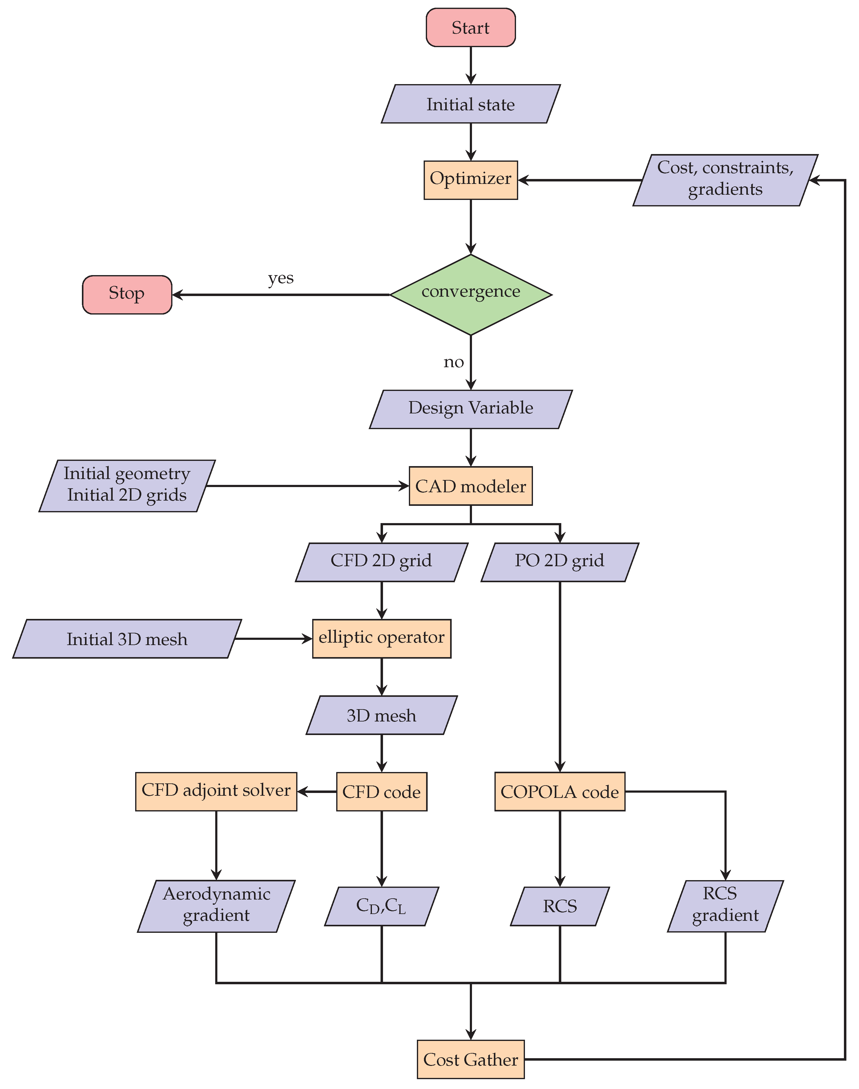
This paper is organized as follows. In Figure 1, the flow chart of the gradient-based aero-stealth coupled optimization is demonstrated, and some numerical methods used in this work are described. Next, the results of the code validation are shown in Section 3 and the problem formulation, baseline geometry of the flying wing, meshes and shape design variables are introduced in Section 4 and Section 5. In Section 6, the accuracy of the sensitivities is tested. After that, in Section 7, a Pareto front is showcased and particularly interesting geometries are highlighted. Finally, in Section 8, we discuss the conclusions based on the results.

2. Methodology

2.1. The Physical Optics Approximation

In an aircraft, stealthiness can mean a number of different things. Here, we will understand it as the capacity of the aircraft to scatter a limited amount of energy back into the direction of the emitter. We consider a monostatic radar, which represents the large majority of the systems in use. This means that the emitting antenna and the receiving antenna are collocated. A popular measure of the scattered electromagnetic energy is the radar cross-section (RCS)

σ

defined as follows :

σ (θ, ϕ) = lim_{R \to \infty} R^{2} \frac{| E_{P} |^{2}}{| E_{i} |^{2}},

(1)

where

E_{P}

is the scattered electric fields at a point

P (R, θ, ϕ)

in polar coordinates and

E_{i}

is the incident electric field at the target, whose norm is considered to be 1

V / m i

n practice. Usually, the RCS is expressed in decibels :

σ_{dB} = 10 log 10 (σ) .

We will restrict this study to radar bands L (1-5 GHz, used for moderate distance surveillance) through X (around 10 GHz, used for missile guidance systems). These frequency bands will produce on a target the size of an aircraft a predominantly high-frequency scattering [1]. Thus, an asymptotically exact method such as a Boundary Element Method (BEM) or Fast Multipole Method (FMM) would be too expensive for an optimization process. Physical Optics (PO) is one of the most common high frequency approximate method for RCS prediction. It is much cheaper than BEM, and it gives a better prediction than a purely optical approximation [20].

For such frequencies, the size of the aircraft is large with respect to the wavelength. Another reasonable assumption is that the distance between the aircraft and the radar antenna is also large with respect to the wavelength, so that the incident electric field can be considered a plane wave, and with respect to the size of the aircraft, so the far field Green’s function approximation to the Stratton-Chu [21] integral equation is valid. Together with a tangent plane approximation, those can be simplified and the scattered electric field

E_{P}

at a point P can be expressed as :

E_{P} = - j \frac{k Z_{0}}{4 π} \frac{e^{- j k R}}{R} \int_{S} u_{s} \times (u_{s} \times J) exp (j k R \cdot (u_{i} - u_{s})),

(2)

with

j = \sqrt{- 1}

, k the wave number,

Z_{0}

the impedance of free space, S the surface of the target,

u_{i}

and

u_{s}

the unit direction vectors for the incident and scattered fields respectively,

R = \vec{O P}

and

R = | R |

, and where J is the surface current density vector. In the PO approximation,

J = \{\begin{matrix} \frac{2}{Z_{0}} n \times u_{i} \times E_{i} & in the illuminated zone, \\ 0 & in the shadow zone, \end{matrix}

(3)

where

n

is the local normal unit vector to the surface.

Note that by (2) that

E_{P} = O (\frac{1}{R}) as R \to \infty .

Therefore, the RCS does not depend on the range.

Although this approximate method does not account for diffraction, and in particular wedge diffraction, extensions exist to correct the induced current along wedges. One such extension is called Partial Theory of Diffraction (PTD) [22] and has been added to PO to give a better prediction of the RCS of an angular shape, such as the trailing edge of a wing.

The solver including PO and PTD along with their differentiation, described on the next section, is dubbed COPOLA.

2.2. Automatic Differentiation of Physical Optics

If the characteristics of the radar wave (wavelength, polarization and direction) are given, the RCS depends only on

x_{e}

the coordinates of the vertices of the surface grid used for the electromagnetism problem.

F_{e} (ν) = {\hat{F}}_{e} (σ (x_{e} (ν)))

is a function depending explicitly only on the RCS

σ

, then the directional derivative of

F_{e}

with respect to a set of geometric variables

ν

(e.g. sweep angle, chord length...) is :

d F_{e} = {\hat{F}}_{e}^{'} (σ) \cdot σ^{'} (x_{e}) \cdot x_{e}^{'} (ν) \cdot d ν .

(4)

We used the Automatic Differentiation (AD) tool TAPENADE [8] in order to generate a differentiated program from the original code which is able to compute the terms

d F_{e} / d σ

and

d σ / d x_{e}

. With this tool, it is possible to save a lot of development and debugging time. TAPENADE offers two modes : tangent (or direct) and reverse.

Tangent mode compute the directional derivative of

F_{e}

in the direction

d ν

using the chain rule, from left to right. This mode is immediate to use as it only needs to create a copy of the input code, interleaved with the derivative instructions. Reverse mode is an efficient way of computing the gradient of

\nabla F_{e} \cdot d ν = d ν^{*} \cdot x_{e}^{'} {(ν)}^{*} \cdot σ^{'} {(x_{e})}^{*} \cdot \hat{F} e^{'} {(σ)}^{*}

. When

F_{e}

is scalar-valued and the dimension of

ν

is large, and assuming that the storage capacity is available, it is theoretically more efficient to compute the Jacobian matrix

\nabla F_{e}

F_{e}

row by row and then compute

d F_{e} = \nabla F_{e} d ν

than to compute it by the chain rule with the tangent mode.

Here, however, all the step of the chain rule computation are cheap to compute since they do not require to solve a system. Therefore, the actual gain in efficiency from the reverse mode is expected to be small, and since it is much more difficult to implement than the tangent mode, we did not deem it worth the trouble.

The term

d x_{e} / d ν

, that is the derivative of the vertex coordinates of the surface grid with respect to a set of geometric variable, is computed by the CAD modeler (see §4.1) and is given as an input to the differentiated PO program.

This allows us to compute the cost function

F_{e}

as well as its derivative

d F_{e} / d ν

in a single call of the PO code.

2.3. The aerodynamic solver

Our in-house Navier-Stokes AETHER code [18,23] solves the 2D, axisymmetric and 3D compressible Navier-Stokes equations. It uses a finite element approach, based on a symmetric form of the equations written in terms of entropy variables. The advantages of this change of variables are numerous: in addition to the strong mathematical and numerical coherence they provide such as dimensionally correct dot product, symmetric operators with positivity properties and efficient preconditioning, entropy variables yield further improvements over the usual conservation variables, in particular in the context of chemically reacting flows.

The code can handle the unstructured mixture of numerous types of elements (triangles and quadrilaterals in 2D; tetrahedral, bricks and prisms in 3D).

Several one- and two-equation Reynolds-averaged turbulence models are available: Spalart-Allmaras, (k,

ε

), (k,

ω

), (k, kl), DRSM… Additional equations devoted to the evaluation of the laminar-turbulence transition can be activated. These models are integrated down to the wall. Extensions to DES and LES are also available.

The linearization of Navier-Stokes equations and turbulence equations requires the differentiation of all the routines involved in the aerodynamic computation. These differentiated routines have been obtained using an Automatic Differentiation tool, TAPENADE. This tool provides the differentiated Fortran routines with respect to input variables prescribed by the user.

We used a compressible Reynolds-Averaged Navier Stokes [24] method with the Spalart-Allmaras [25] turbulence model in order to compute the aerodynamic criterion and constraints.

2.4. Adjoint Approach for CFD

Let W be a vector state solution of the non-linear RANS equation system which we note as

R = 0 .

Finally, let

F_{a}

be an observation function of the field W. For the process of optimization, we need to compute the derivatives

\frac{d F_{a}}{d ξ}

and

\frac{d F_{a}}{d ν}

with respect to a set of aerodynamic variables

ξ

(e.g. the angle of attack) and geometric variables

ν

(e.g. the wing sweep angle) respectively. The variables

ν

and

ξ

are independent of one another.

In order to mitigate the cost of computing the gradient of the aerodynamic criterion with respect to many variables, we use an adjoint approach [26].

When a surface grid of coordinates

x_{a}

is subjected to a deformation thanks to the CAD modeler, the deformation is propagated to the 3D grid of coordinates

X_{a}

with the help of an elliptic operator described by the system :

L (X_{a}, x_{a}) = 0 .

(5)

Let us write

F_{a}

and

R

as functions of

ξ

X_{a}

and W. Note that

ξ

is an independent variable but

X_{a}

depends on

ν

and W depends on both

ξ

and

ν

2.4.1. Gradient with Respect to Aerodynamic Variables

First, the derivative of

F_{a}

and

R

with respect to

ξ

can be written as

d F_{a} = ({\frac{\partial F_{a}}{\partial ξ}|}_{W} + {\frac{\partial F_{a}}{\partial W}|}_{ξ} \frac{\partial W}{\partial ξ}) d ξ,

(6)

and

d R = ({\frac{\partial R}{\partial ξ}|}_{W} + {\frac{\partial R}{\partial W}|}_{ξ} \frac{\partial W}{\partial ξ}) d ξ = 0 .

(7)

The term

\frac{\partial W}{\partial ξ}

in (6) is not easy to compute in itself, but it can be expressed differently thanks to (7) :

\frac{\partial W}{\partial ξ} = - {({\frac{\partial R}{\partial W}|}_{ξ})}^{- 1} {\frac{\partial R}{\partial ξ}|}_{W} .

(8)

Consequently, (6) can then be written as :

d F_{a} = ({\frac{\partial F_{a}}{\partial ξ}|}_{W} - Ψ^{T} {\frac{\partial R}{\partial ξ}|}_{W}) d ξ .

(9)

Where

Ψ

is the solution to the aerodynamic adjoint system :

{({\frac{\partial R}{\partial W}|}_{ξ})}^{T} Ψ = {({\frac{\partial F_{a}}{\partial W}|}_{ξ})}^{T} .

(10)

2.4.2. Gradient with Respect to Geometric Variables

The derivative of

R

and

F_{a}

with respect to

ν

are :

d F_{a} = ({\frac{\partial F_{a}}{\partial X_{a}}|}_{W} \frac{\partial X_{a}}{\partial ν} + {\frac{\partial F_{a}}{\partial W}|}_{X_{a}} \frac{\partial W}{\partial ν}) d ν,

(11)

and

d R = ({\frac{\partial R}{\partial X_{a}}|}_{W} \frac{\partial X_{a}}{\partial ν} + {\frac{\partial R}{\partial W}|}_{X_{a}} \frac{\partial W}{\partial ν}) d ν = 0 .

(12)

As in Section 2.4.1, we can express the term

\frac{\partial W}{\partial ν}

of equation (11) thanks to (12) as :

\frac{\partial W}{\partial ν} = {({\frac{\partial R}{\partial W}|}_{X_{a}})}^{- 1} {\frac{\partial R}{\partial X_{a}}|}_{W} \frac{\partial X_{a}}{\partial ν},

(13)

and then :

d F_{a} = ({\frac{\partial F_{a}}{\partial X_{a}}|}_{W} - Ψ^{T} {\frac{\partial R}{\partial X_{a}}|}_{W}) \frac{\partial X_{a}}{\partial ν} d ν,

(14)

where

Ψ

is the same as defined in equation (10).

The work is not yet done, though, as the term

\frac{\partial X_{a}}{\partial ν}

is not to compute. In order to find a more convenient expression, we must write the derivative of

L

with respect to

ν

d L = ({\frac{\partial L}{\partial X_{a}}|}_{x_{a}} \frac{\partial X_{a}}{\partial ν} + {\frac{\partial L}{\partial x_{a}}|}_{X_{a}} \frac{\partial x_{a}}{\partial ν}) d ν,

(15)

and then once again we can express the term

\frac{\partial X_{a}}{\partial ν}

as a function of more convenient derivatives :

\frac{\partial X_{a}}{\partial ν} = {({\frac{\partial L}{\partial X_{a}}|}_{x_{a}})}^{- 1} {\frac{\partial L}{\partial x_{a}}|}_{X_{a}} \frac{\partial x_{a}}{\partial ν},

(16)

which finally yields :

d F_{a} = - Φ^{T} {\frac{\partial L}{\partial x_{a}}|}_{X_{a}} \frac{\partial x_{a}}{\partial ν} d ν,

(17)

where

Φ

is solution of the mesh adjoint equation system :

{({\frac{\partial L}{\partial X_{a}}|}_{x_{a}})}^{T} Φ = {({\frac{\partial F_{a}}{\partial X_{a}}|}_{x_{a}})}^{T} - {({\frac{\partial R}{\partial X_{a}}|}_{x_{a}})}^{T} Ψ .

(18)

2.4.3. Summary

F_{a}

is an observation depending on W, then the derivative of

F_{a}

with respect to a set of geometric variables

ν

and respectively to a set of aerodynamic variables

ξ

can be written as :

\begin{matrix} \frac{d F_{a}}{d ν} & = - Φ^{T} \frac{\partial L}{\partial x_{a}} \frac{\partial x_{a}}{\partial ν}, \end{matrix}

(19)

\begin{matrix} \frac{d F_{a}}{d ξ} & = \frac{\partial F_{a}}{\partial ξ} - Ψ^{T} \frac{\partial R}{\partial ξ}, \end{matrix}

(20)

where

x_{a}

is the coordinates of the 2D mesh for the aerodynamic problem,

X_{a}

is the coordinates of the 3D aerodynamic mesh and

Φ

is the mesh adjoint, solution of :

{(\frac{\partial L}{\partial X_{a}})}^{T} Φ = {(\frac{\partial F_{a}}{\partial X_{a}})}^{T} - {(\frac{\partial R}{\partial X_{a}})}^{T} Ψ,

(21)

with

Ψ

the aerodynamic adjoint, solution of :

{(\frac{\partial R}{\partial W})}^{T} Ψ = {(\frac{\partial F_{a}}{\partial W})}^{T} .

(22)

3. Validation

3.1. Validation of the COPOLA Code

We used a sphere geometry as a test case for the validation of COPOLA. According to Mie’s theory, if a sphere of radius R is illuminated by a wave of wavelength

λ

, then the RCS

σ

converges to the section area of the sphere as the wavelength decreases :

lim_{λ \to 0} σ = π R^{2} .

Moreover, due to the symmetric properties of the sphere, its RCS does not depend on the bearing angle.

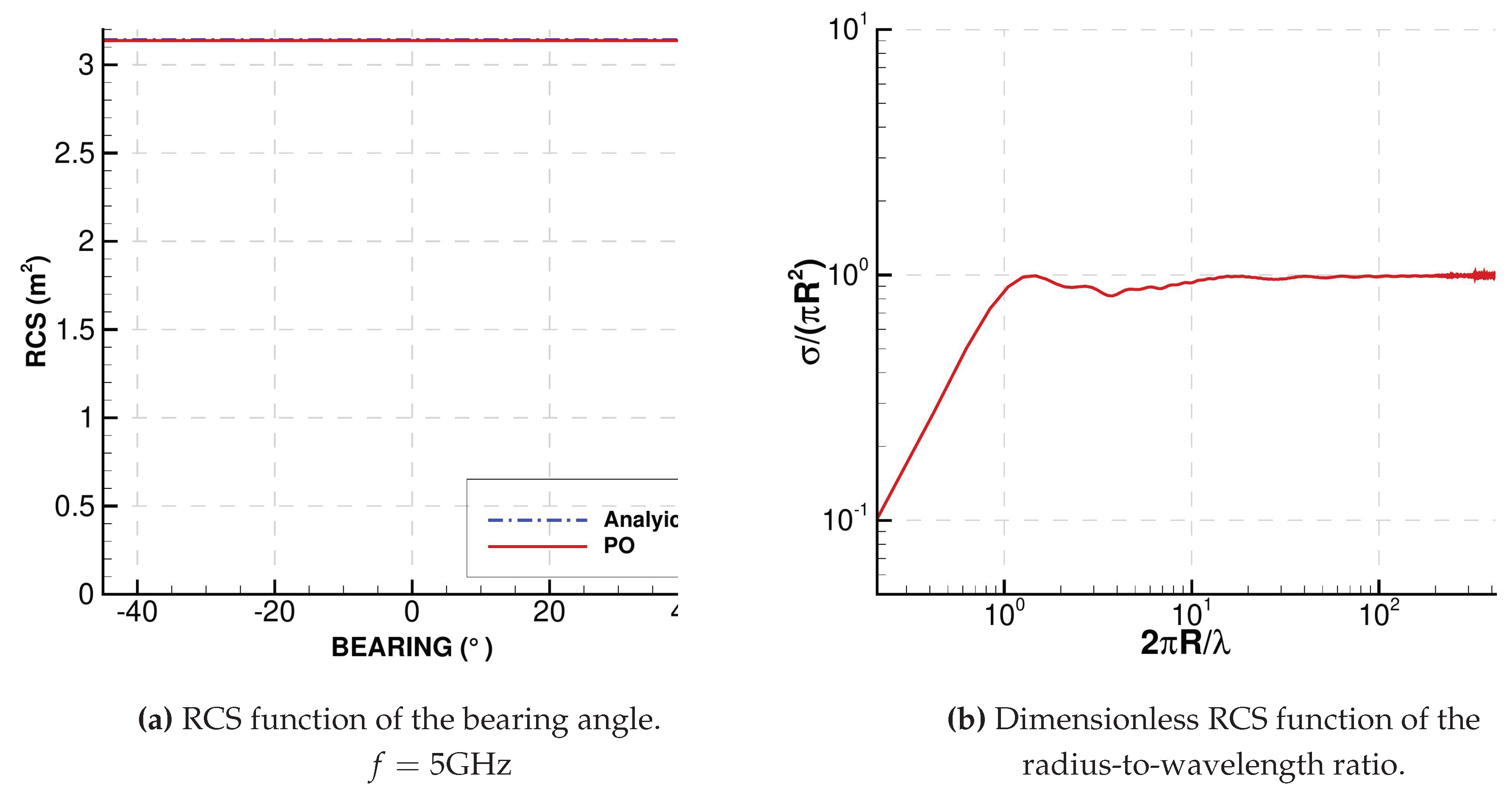
Since PO method is a high frequency approximation, it should predict an RCS close to the analytical value. Figure 3 shows the PO prediction of the RCS of a sphere of radius 1 m with respect to the bearing angle (Figure 3a) and frequency (Figure 3b). The plot in Figure 3b has been computed with 2000 frequencies between

10 M Hz

and

20 G Hz

In Figure 3a, the RCS is independent on the bearing angle, as it should be, and the error to the analytical value is around 0.15%. Figure 3b shows that, when the frequency is too low (

\frac{2 π f R}{c} < 50

, with c the speed of light), the predicted RCS is very far from the analytical value, and the PO approximation is not trustworthy. When the frequency is too high (

\frac{2 π f R}{c} > 100

), the prediction starts to deteriorate again, due to the mesh being too coarse for the higher frequencies.

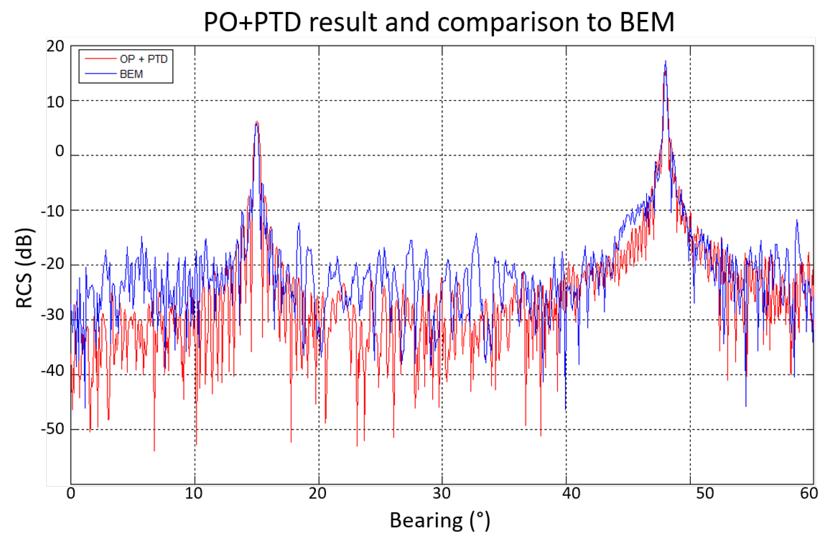
Figure 4 shows the comparison between an RCS simulation and a BEM computation on the GFA geometry (described on Section 4). The BEM computation was performed thanks to the SPECTRE solver [27,28].

PO is able to predict accurately both the height and the width of the two main peaks. Away from of these peaks, the RCS is very low (around

- 20

). The precision of PO is not as good in these zones because low frequency effects such as creeping waves are predominant, but since the RCS is so much lower than that of the peaks, it is negligible for the purpose of this study.

4. Baseline Description

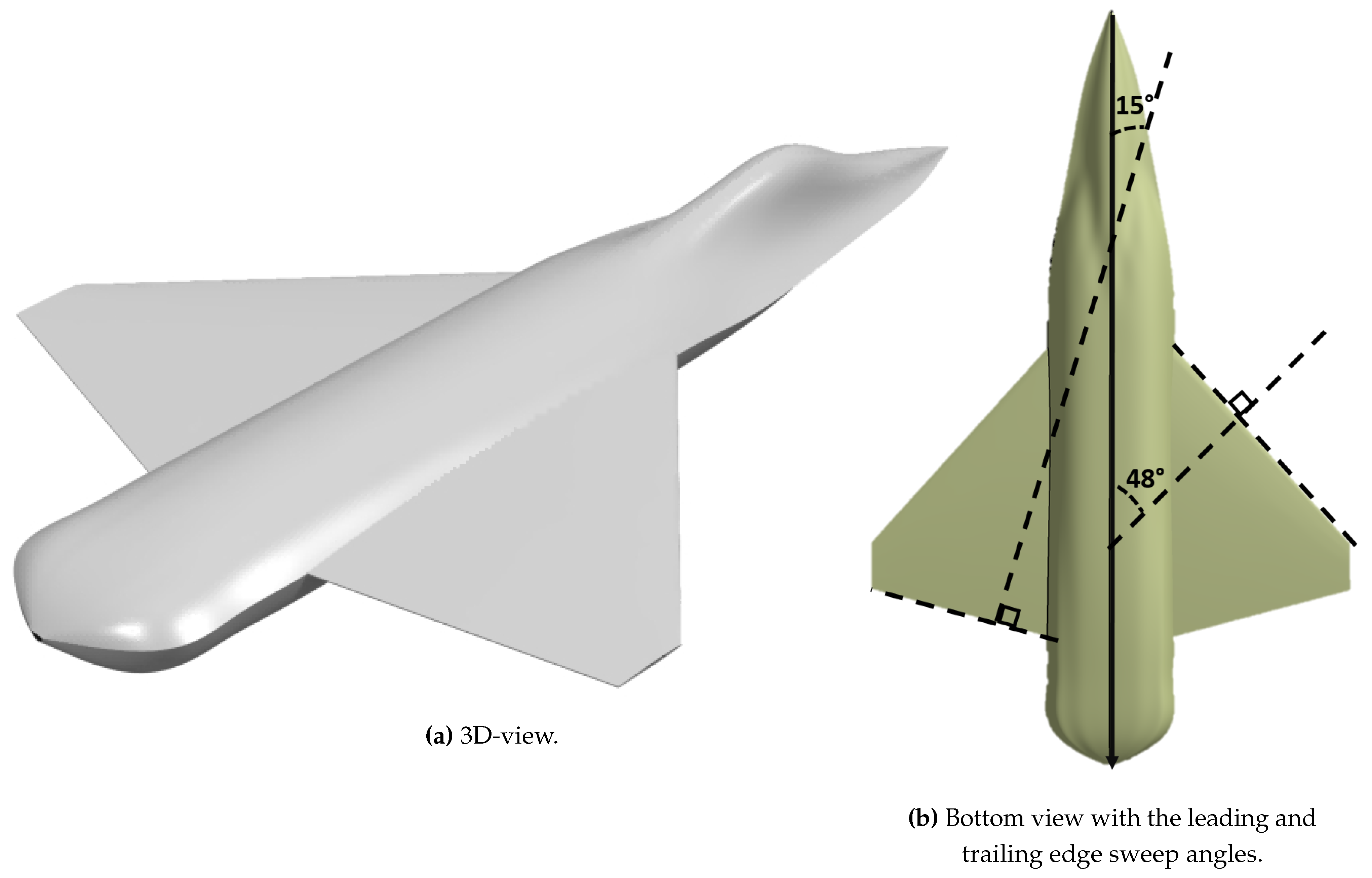
The geometry we use is a simplified shape of a Generic Fighter Aircraft (GFA, see Figure 5). It features the fuselage without air intake, and a pair of wings. The wings have a trapezoidal shape, without leading edge extension. It does not have a tail fin, horizontal stabilizer or canard. The front of the fuselage has a ridge on both side. We did not use a realistic geometry for the rear of the fuselage, so the physics of the wake will not be accurately represented. Since we only performed supersonic simulations, this will not disturb the flow upstream. This also allows us to be lenient with meshing the downstream region, thus saving computation time.

4.1. The CAD Modeler

In order to model and modify the geometry, we use the CAD tool GANIMEDE [17]. In this study, we used some functionalities of GANIMEDE that have not yet been differentiated, which prevented us from using the exact differentiation presented in [17]. The surface is represented by a set of NURBS grids and parametrized with control points. GANIMEDE uses both global and local variables as input. Local variables are the osculating parameters (i.e. position, tangent and curvature) at a control point. Global variable allow us to modify usual aeronautical design variables such as sweep and twist angles, or the chord of a wing. In this study, we used only global variables.

If a surface mesh is associated to the baseline geometry, GANIMEDE will project the mesh onto the deformed geometry, and compute the derivatives of the mesh node coordinates with respect to the design variables

\frac{d x}{d ν}

using centered finite difference. Because of the smoothing and other refinement operations performed by the CAD modeler on the NURBS geometry, too small a step size can lead to a bad gradient, so we have to find an optimal step size for each design variable.

4.2. Aerodynamic Analysis of the Baseline

We performed a CFD simulation of the GFA geometry. The upstream Mach number is 1.8, with an angle of attack of 2

°

. The overall drag coefficient is

387.5

drag count and the lift coefficient is

0.113

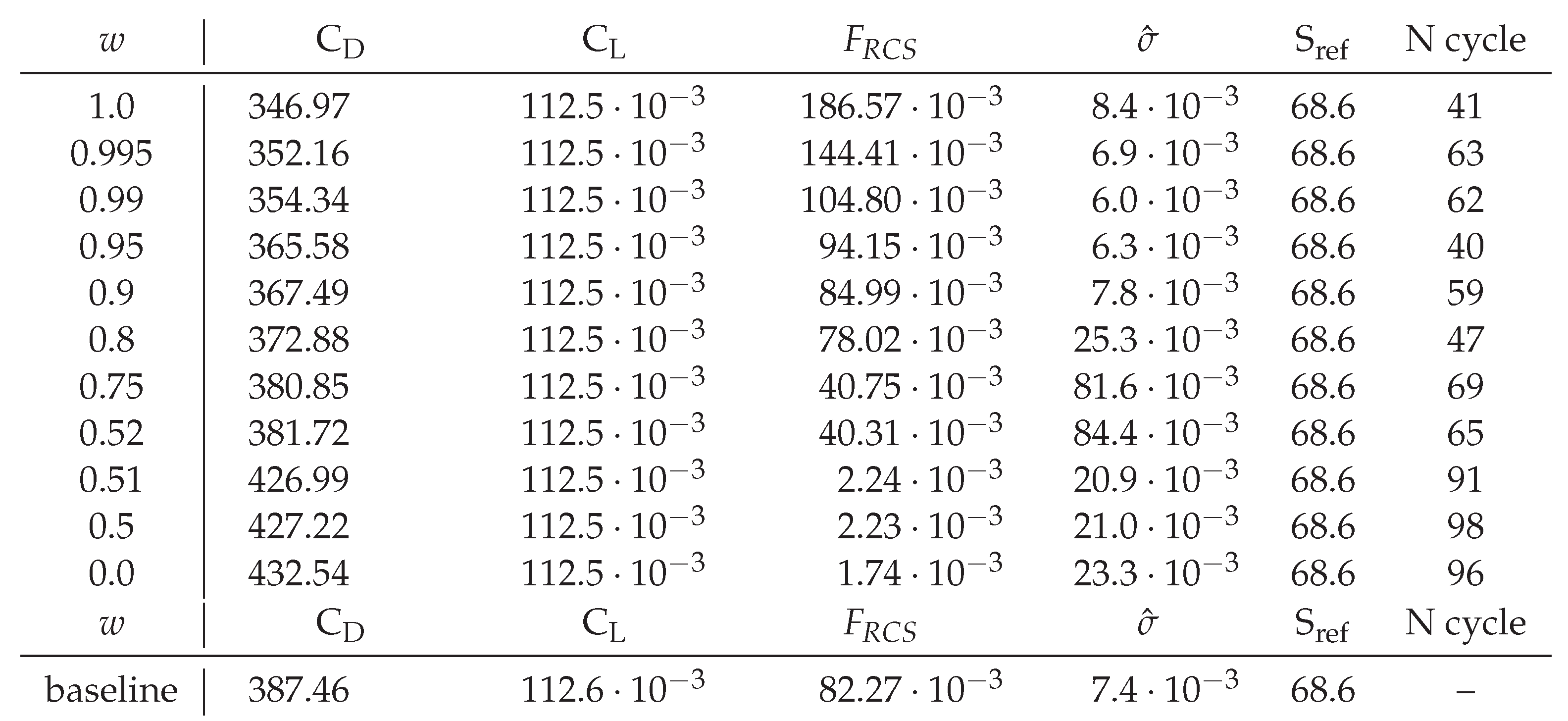
. These values are gathered in Table 1.

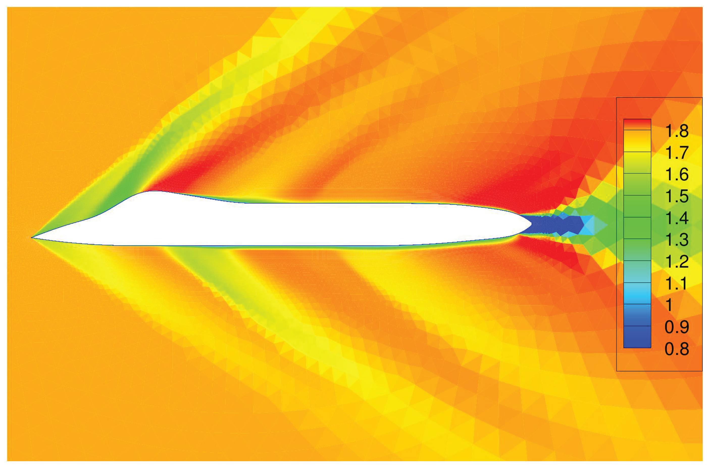
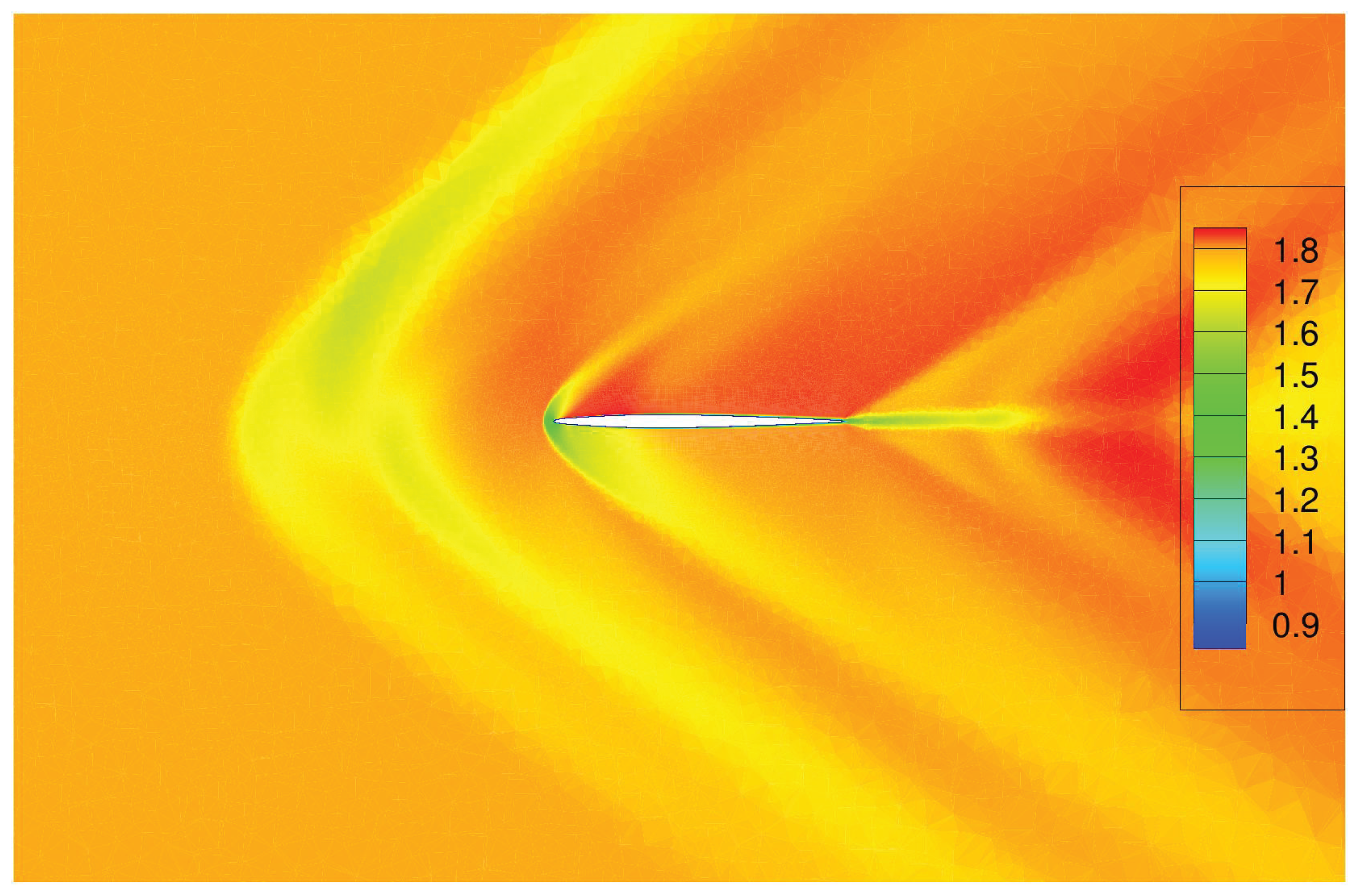
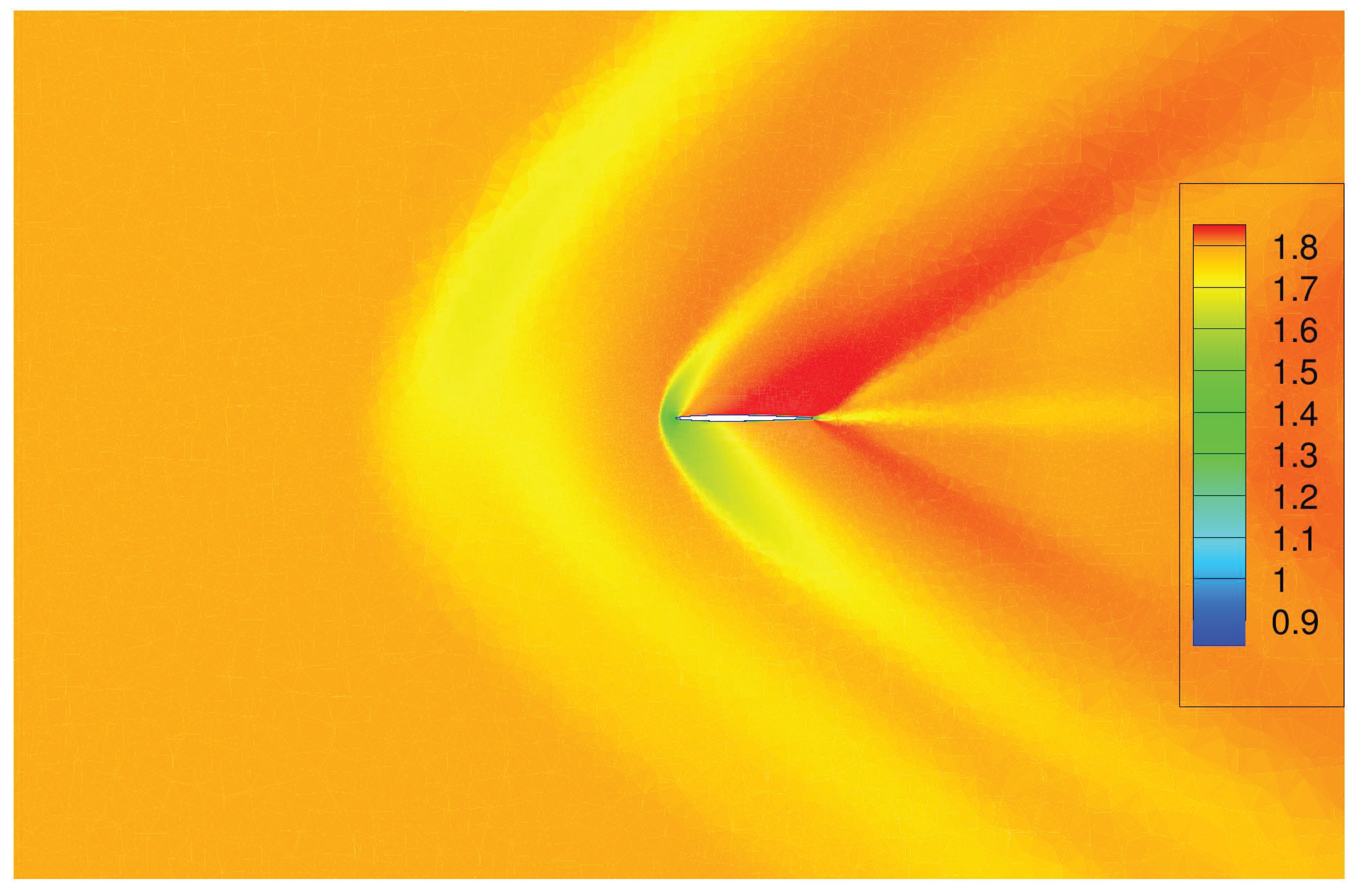
The field of local Mach number in the symmetry plane and in the planes parallel to the symmetry plane at

Y / b = 0.45

and

Y / b = 0.8

are displayed in Figure 6,Figure 7 and Figure 8 respectively.

In the symmetry plane (Figure 6), we can clearly see the weak, attached shock on the nose of the GFA. A large detached area is present at the rear of the aircraft, which is expected since no attention was directed towards this area.

In Figure 7 and Figure 8, directly upstream of the wing leading-edge, we can see a weak bow shock.

4.3. Stealth Analysis of the Baseline

The span of the baseline shape being

6 m

, the frequency should be higher than

25 M Hz

in order to meet the criterion of Section 3.1:

50 < \frac{2 π f L_{r e f}}{c} < 100

The COPOLA simulation is done on a range of bearing angles from 0 to

70^{°}

with a step of

0 . 01^{°}

and on a range of elevation angles from -20 to

- 10^{°}

with the same step, in order to simulate an aircraft reflecting hostile waves from a radar on the ground far in front of the plane. For each line of sight, the simulation is run for 11 frequencies around a main frequency at

1 G Hz

} and spanning

100 M Hz

}. The step for the bearing and elevation angles has been chosen according to the Shannon criterion.

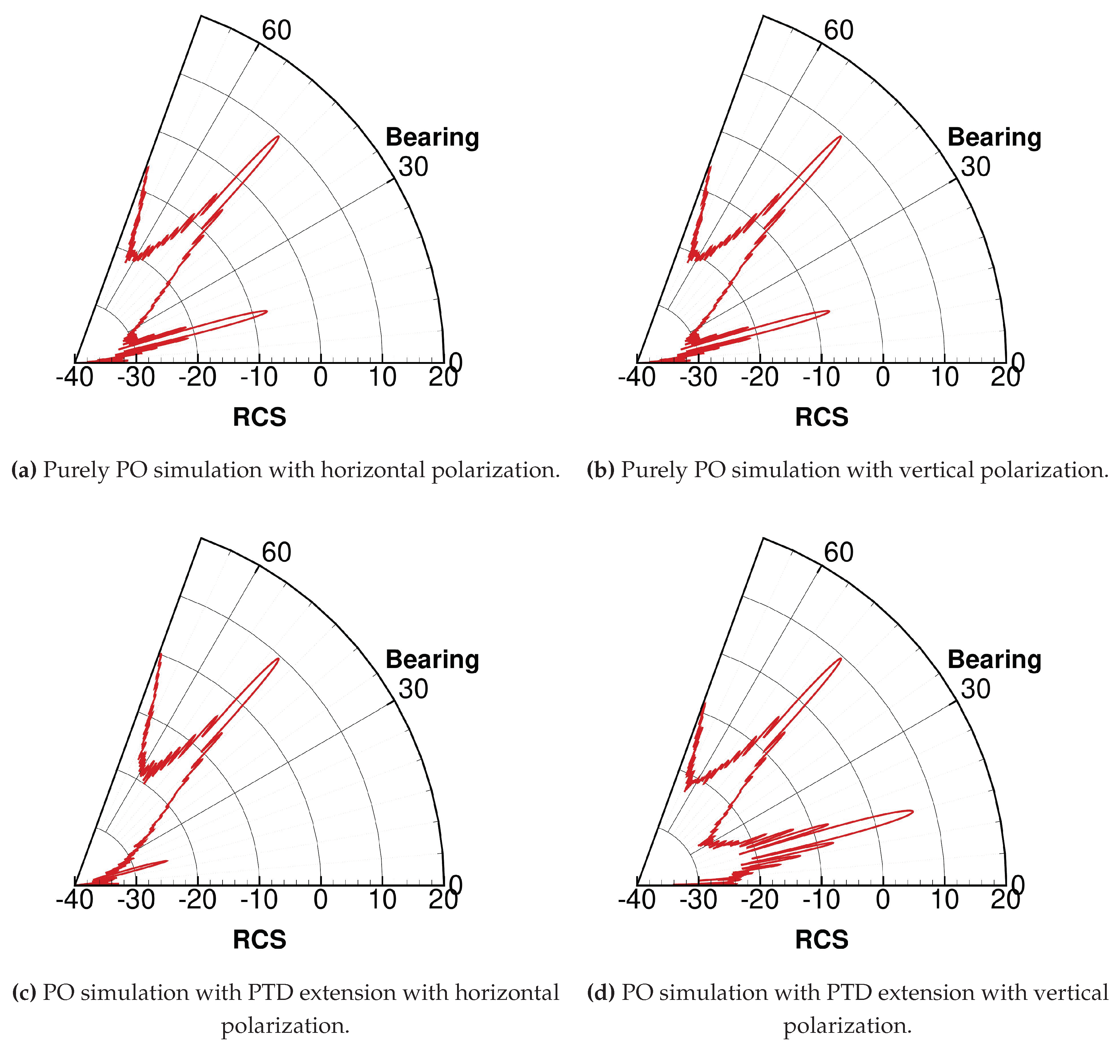
In Figure 9b and Figure 9a, a peak is visible around

48^{°}

of bearing. This corresponds to the direction the leading edge is facing. This peak is the specular reflection of the incident wave onto the leading edge. A second peak appears at around -15

°

. This peak has a much lower intensity compared to the specular reflection peak, due to the non-continuity of the normal at the trailing edge wedges. Physically, this means that the trailing edge wedges diffract the incident wave. However, the peak appears to have the same intensity no matter the polarization, which, given the orientation of the trailing edge (see Figure 5) should not be the case : the trailing edges being horizontal, the diffraction should be negligible when observed with a horizontal polarization [29]. We conclude that PO alone is not enough to compute the trailing edge diffraction, and we need to add the PTD extension to our simulation to adequately predict the RCS. When taking diffraction into account, the second peak appears much brighter with the vertical polarization (Figure 9c), only a few dB less intense than the specular reflection peak, and it is almost absent with the horizontal polarization (Figure 9d).

Over the rest of the observation window, the RCS is very low, around -30 to -20 dB, which is practically negligible, but increases as the bearing angle comes close to

70^{°}

. This is likely due to the influence of the fuselage, but as it is far away from the axis of the plane, it is not relevant to this study. One might note however that the value around

70^{°}

is not the same with or without the PTD extension. This is likely due to a diffraction by the wing tip of by wedges on the fuselage that are overestimated by PO alone.

Since the vertical polarization is strictly richer than the horizontal polarization in our case, it is the one we will be using for RCS simulation in the rest of this study.

4.4. Optimization Parameters

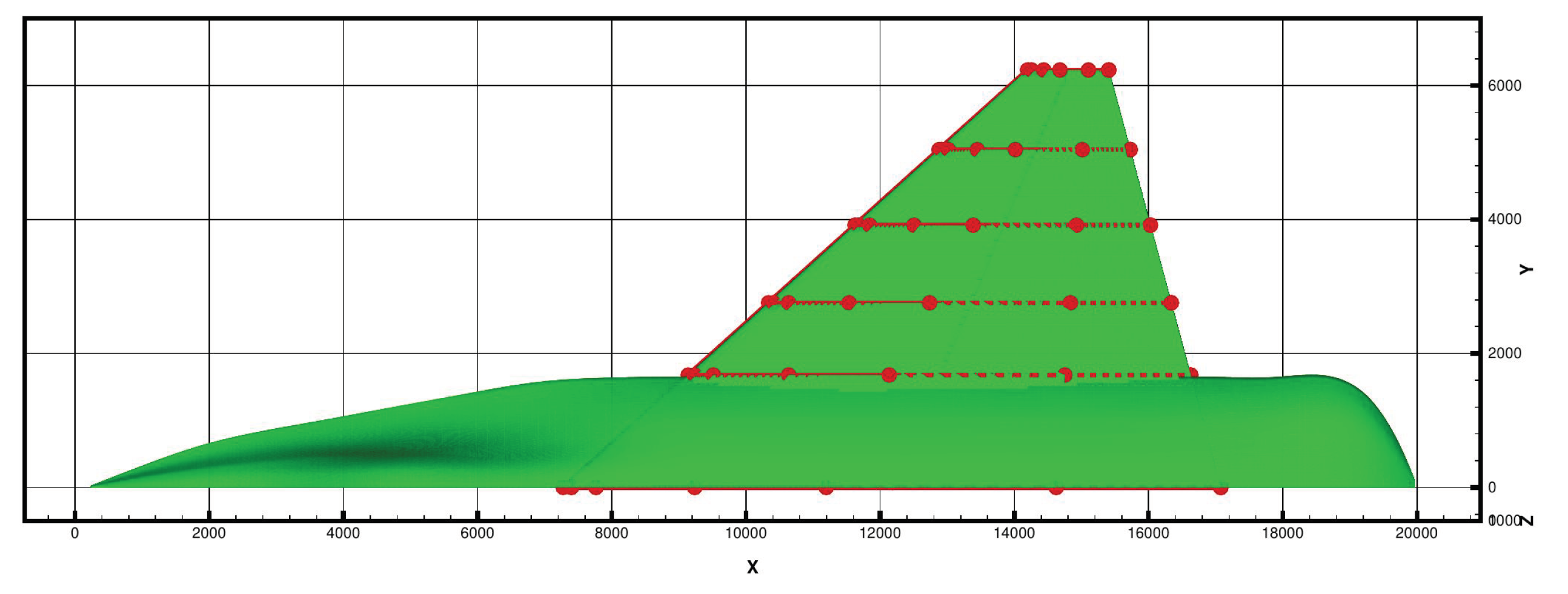
The wing of the GFA is parametrized with the help of 6 control sections, with 15 control points along each of them (see Figure 10). All the section are and will stay parallel to the symmetry plane. Section number 1 is at the symmetry plane and won’t be modified. Section 2 is a few centimeters away from the root of the wing. At section 4, continuity of the tangent is not ensured, allowing for a sharp angle on the wing. The fuselage is not modified.

The geometry is parametrized with the help of 13 global variables :

the leading edge sweep angle the section 2 and 4,
the chord of section 2, 4 and 6,
the distance between section 2 and 6,
the twist angle of section 2, 3, 5 and 6,
the leading edge camber of section 3, 5 and 6.

The chords of section 3 and 5 are interpolated between that of section 2 and 4 and 6 respectively. The twist angle for a given section is a rotation along an axis perpendicular to the section going through a point at 25% chord and 50% thickness. Both the leading edge camber and the twist angle at section 4 are interpolated between sections 3 and 5.

Finally, the angle of attack is the 14 optimization parameter. It is a private to the aerodynamic process.

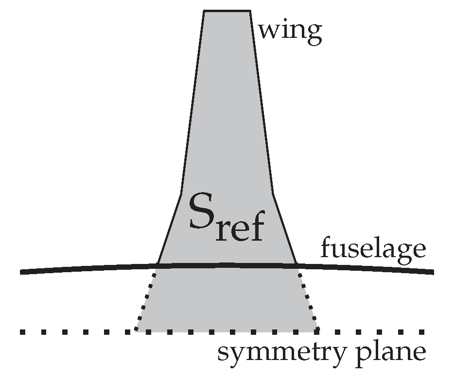
Figure 11. Definition of S_ref

5. Cost and Constraints

In order to explore multiple tradeoffs between aerodynamic and stealth optima, we define the cost function as a weighed sum of an aerodynamic criterion and a stealth criterion :

F = w F_{a} + (1 - w) F_{e},

(23)

with

0 \leq w \leq 1

5.1. Aerodynamic Criterion

For the aerodynamic optimization, we minimize the drag coefficient (

C_{D}

) :

F_{a} = \frac{C_{D}}{{C_{D}}^{r e f}} .

(24)

This is somewhat simplistic, and will lead to unrealistic shapes. Practically, a criterion based on the pitching moment coefficient should be added to the drag criteria, as well as a criterion based on the rolling stability or maneuverability.

However, since the goal of this study is to showcase the methodology rather than find a realistic shape, we will settle for this simplified criterion.

5.2. Stealth Criterion

Typically, a stealth aircraft shape is designed to scatter radar wave away from any hostile radar antenna, which is usually located roughly in front of the aircraft, slightly below. For example, the upward facing planes of the F117 scatter the radar wave into the sky, while more modern aircraft, like the B2, are built to concentrate the reflected radar wave only as a very narrow signal in a few specific directions ("peak directions"). The stealth criterion is built to reflect and favor this behavior : we want to minimize the RCS in every direction in a given sector

(θ_{0}, θ_{1}) \times (ϕ_{0}, ϕ_{1})

, except for a limited interval around a peak direction where the RCS can be high.

In order to manage dimensionless quantities, the electromagnetic criterion is defined as follows :

F_{e} = \frac{\tilde{σ}}{{\tilde{σ}}^{r e f}},

(25)

where

\tilde{σ}

is a weighed average of a function of

σ_{dB}

\tilde{σ} = \int_{θ_{0}}^{θ_{1}} \int_{ϕ_{0}}^{ϕ_{1}} Γ_{d} (θ) δ_{s} (σ_{dB}) sin (ϕ) d θ d ϕ .

(26)

The function

δ_{s}

is a differentiable threshold function built to cut the low intensity variations that we noted in Figure 9, that have a negative impact on computation of the gradient of the cost function :

δ_{s} (x) = \frac{x - s}{1 + e^{- τ (x - s)}},

(27)

with

τ

a parameter that allows to control the sharpness of the peak. The threshold

s = - 5 dB

was chosen.

The function

Γ_{d}

is a weighting function chosen to favor the peak directions. It is close to 1 everywhere, except in the neighborhood of the direction d where it decreases quickly :

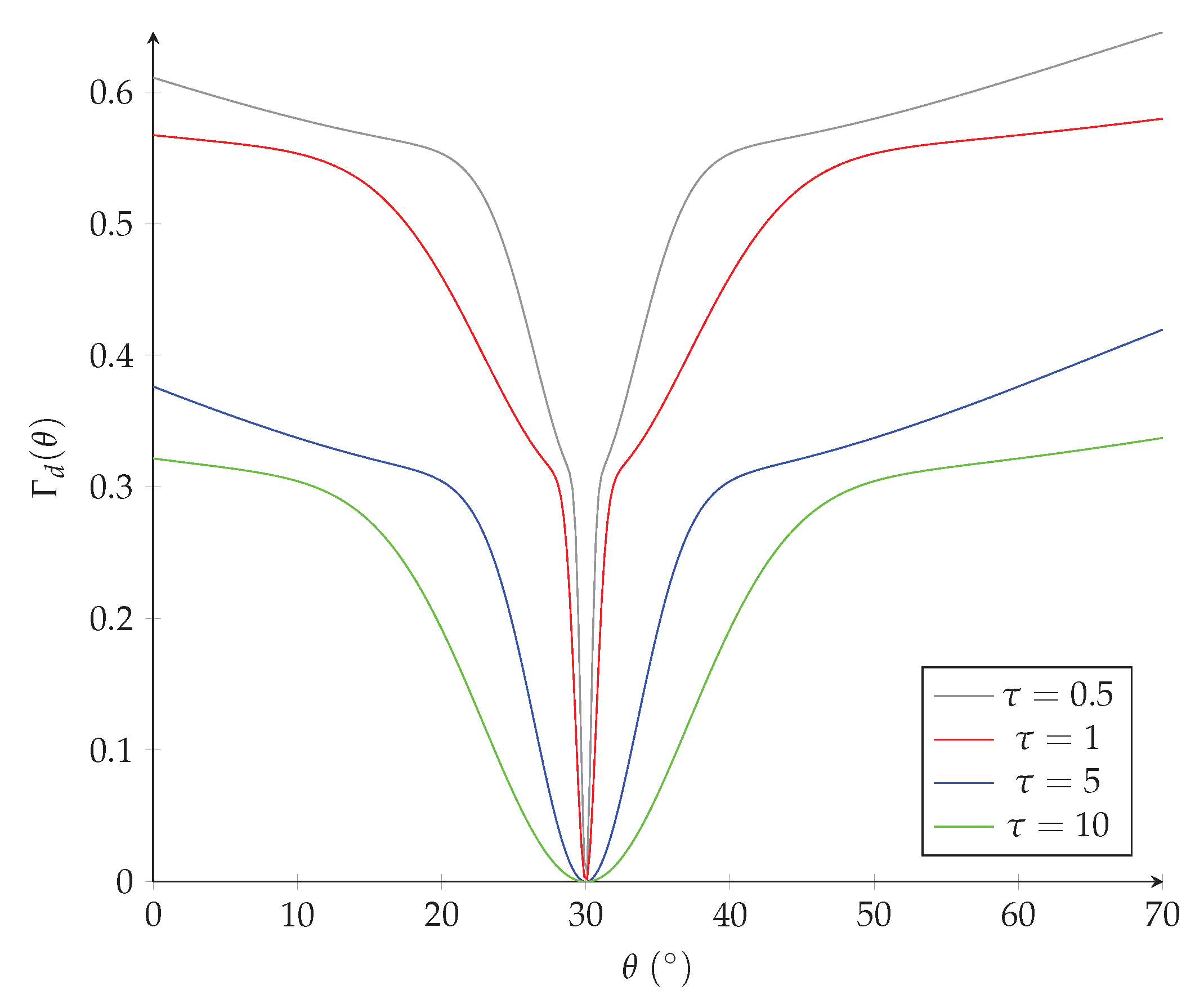
Γ_{d} (θ) = 1 - \frac{1}{2} \sum_{i = 0}^{4} \frac{6 - i}{10} exp (- {(\frac{θ - d}{10^{i} τ})}^{2}) .

(28)

Graphs of the function

Γ_{d}

are shown in Figure 12 for various values of

τ

. For this study, we have chosen, somewhat arbitrarily, a peak direction at a bearing of

d = 30^{°}

, and

τ = 0.1

5.3. Constraints

In order to ensure that the reduced drag coefficient does not come at the cost of a lower lift, we constrain the optimization to work at a constant lift coefficient (

C_{L}

Furthermore, we want to preserve the reference surface (

S_{ref}

) of the wing.

S_{ref}

is defined in Figure 11.

6. Sensitivity Validation

6.1. RCS with Respect to Geometric Variables

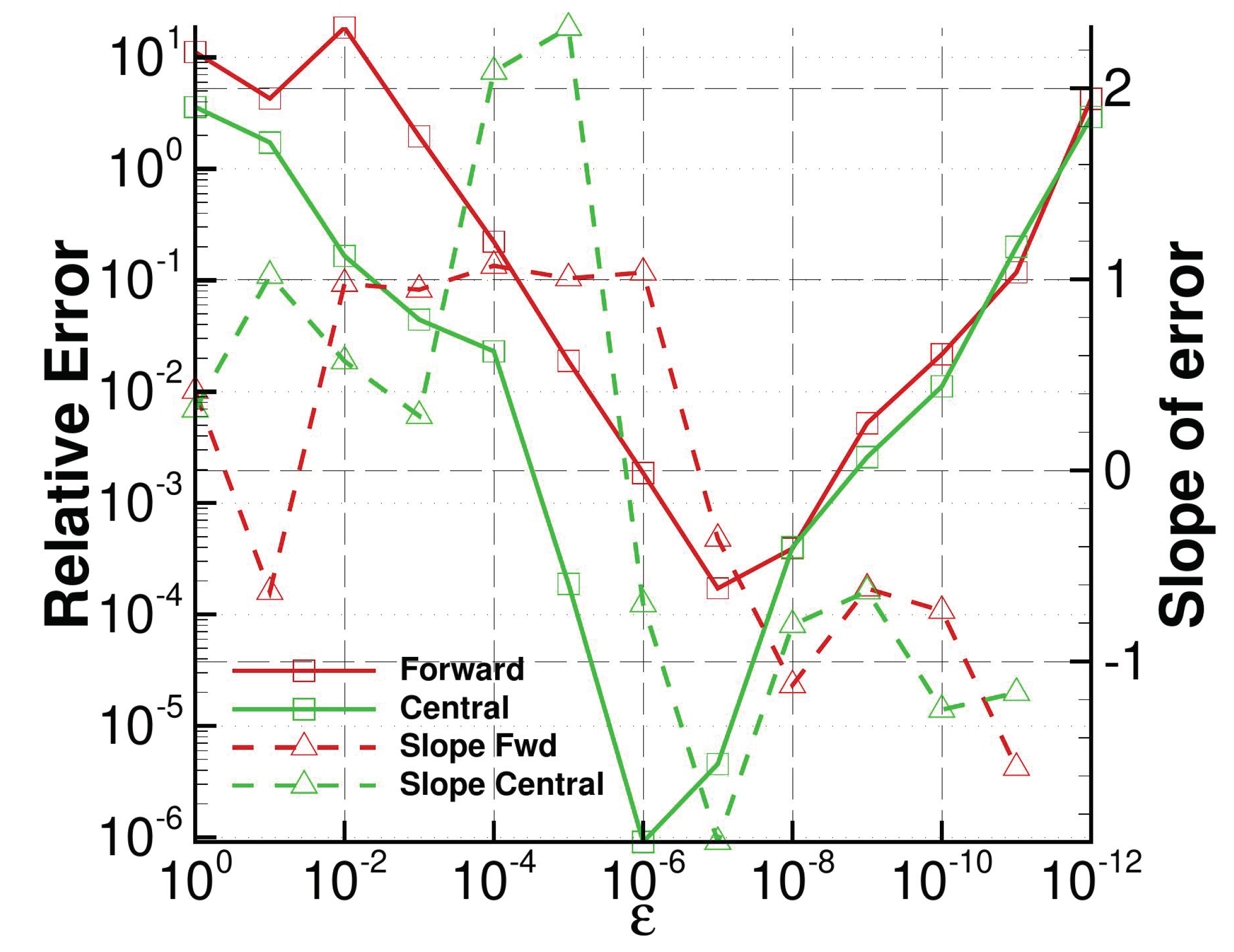
We validated the RCS gradient with respect to the 13 shape design variables by comparing it finite differences (FD) for various step sizes ranging from 1 to

10^{- 12}

, in the unit of each individual variables. For the sake of simplicity, each FD gradient is computed with the same step size for each design variable. In practice of course, we should fine tune a different step size for each individual variable in order to get a more precise gradient.

If the gradient is properly computed, we expect that, if the step size is small enough, the error decreases with the step size, up until a point where the numerical error on the function is of the same order of magnitude as the difference between the values of the RCS function at

ν

and

ν + ϵ \hat{d}

(where

\hat{d}

is an arbitrary direction unit vector). After this critical point, the error should increase roughly linearly as the step size continues decreasing.

Let f denote a real valued function, at least three times differentiable,

f^{'}

its derivative and

Δ_{ϵ} f

and

δ_{ϵ} f

its derivative approximated with respectively forward and centered FD with a step size

ϵ

. It is well known that

\begin{matrix} Δ_{ϵ} f - f^{'} = o (ϵ) & as ϵ \to 0, \end{matrix}

(29)

\begin{matrix} δ_{ϵ} f - f^{'} = o (ϵ^{2}) & as ϵ \to 0 . \end{matrix}

(30)

Hence, the logarithm of the error between the exact gradient and the FD should be linear with respect to the step size if the step size is small enough but bigger than the critical step size, and its slope should be 1 for forward FD and 2 for centered FD. We consider that the minimal error should be at most

10^{- 3}

for forward FD and

10^{- 6}

for centered FD in order to deem the gradient acceptable.

Figure 13 shows the norm of the difference (the solid line) between the gradient computed by COPOLA and the DF gradients function of the step size, for both forward (in red) and centered (in green) difference, as well as the slope of the logarithm of the error (the dashed line).

The forward FD behaves very well : it is linear with a slope of 1 for a wide range of step sizes and the minimal error is a few

10^{- 4}

. The centered difference is also acceptable with a minimal error of around

10^{- 6}

and a slope of 2 right before the critical step size.

6.2. $C_{D}$ with Respect to Geometric and Aerodynamic Variables

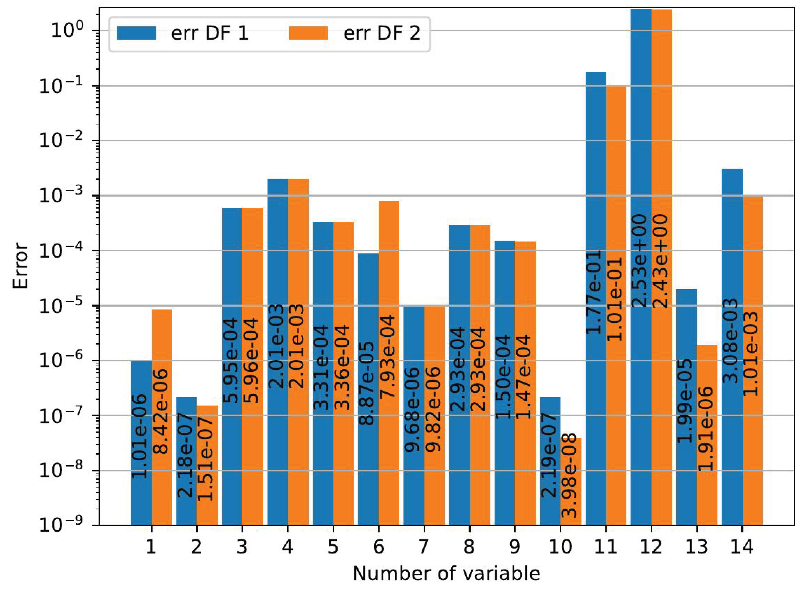
Figure 14 shows the error between the adjoint gradient and the finite differences, both centered and forward, for the optimal step size determined for the CAD gradient. When the value of the adjoint gradient is high enough (more than

10^{- 3}

), the relative error is used :

\frac{| δ F_{a} / δ ν - \partial F_{a} / \partial ν |}{\partial F_{a} / \partial ν} .

When the gradient is too small, the relative error maybe misleading, so the absolute error is used instead :

| δ F_{a} / δ ν - \partial F_{a} / \partial ν | .

Most of the points show a pretty accurate gradient, with an error of at most

10^{- 3}

. The only exceptions are the gradient with respect to the leading edge camber of the 3 and 5 sections. In these cases, the forward and central finite differences are not in good agreement with each other, which indicates that the step size imposed by the CAD gradient is not small enough to compute an accurate aerodynamic gradient.

A more accurate validation of the aerodynamic gradient would be achievable with a methodology similar to that used in Section 6.1 in order to free ourselves from the step size determined by the CAD gradient, but this was not feasible for the CFD code.

7. Optimization Results

7.1. Aerodynamic Optimization

First, we performed an optimization with a purely aerodynamic objective function (

w = 1

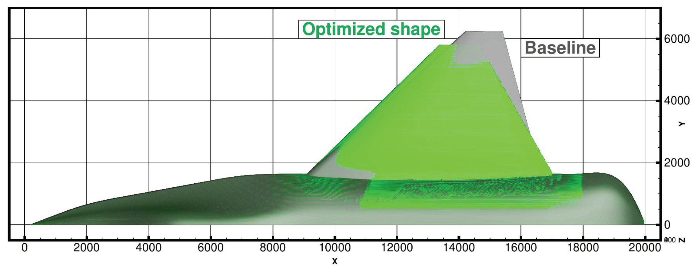
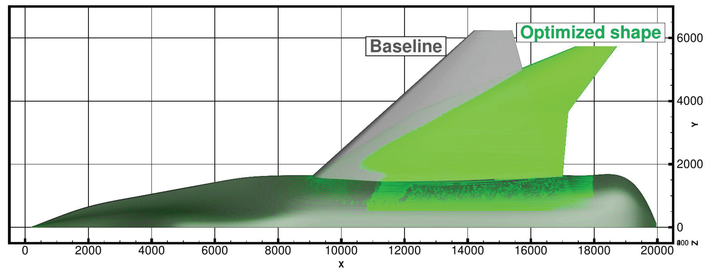
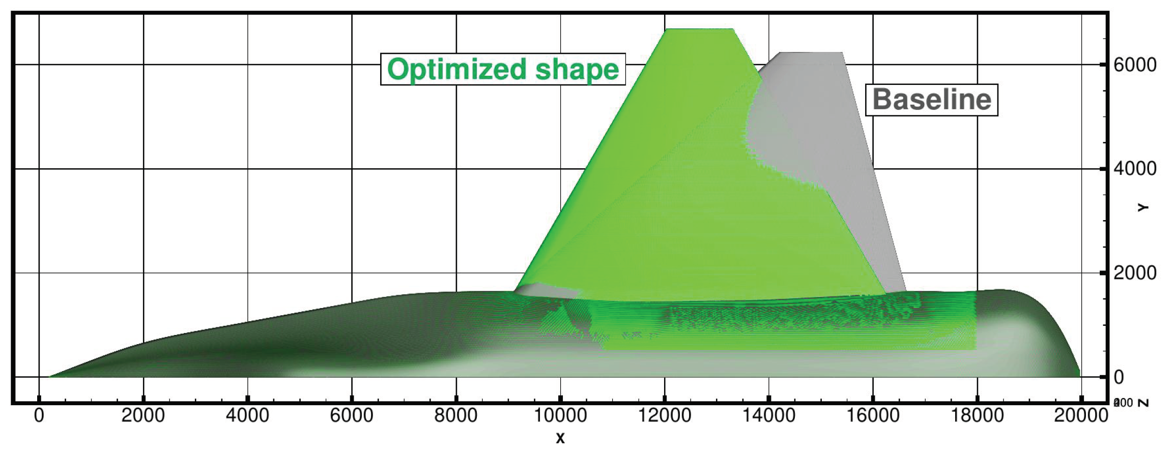
.). The planform of the optimal shape compared to that of the baseline is presented of Figure 15. Most notably, the leading edge sweep angles have reached their respective upper-bounds, leading to an unrealistic shape. As discussed in Section 5.1, this was expected because of a simplistic criterion, relying only on the drag coefficient rather than dealing with any lateral stability criterion. Since the simulation is supersonic, the main contributor to the drag is the wave drag due to the shock waves developing on the nose of the aircraft and the wing leading edge. Increasing the leading edge sweep angle will decrease the shock strength and the wave drag.

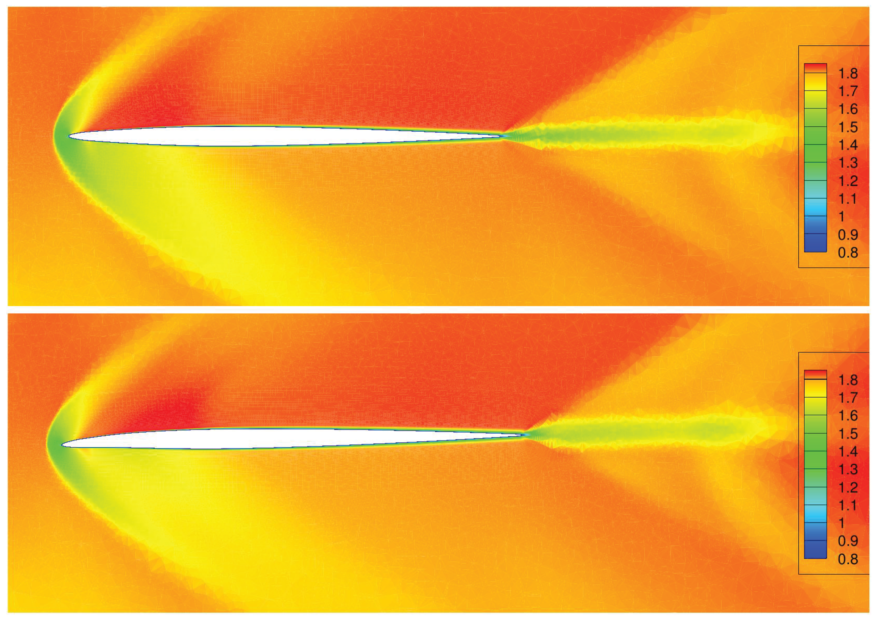
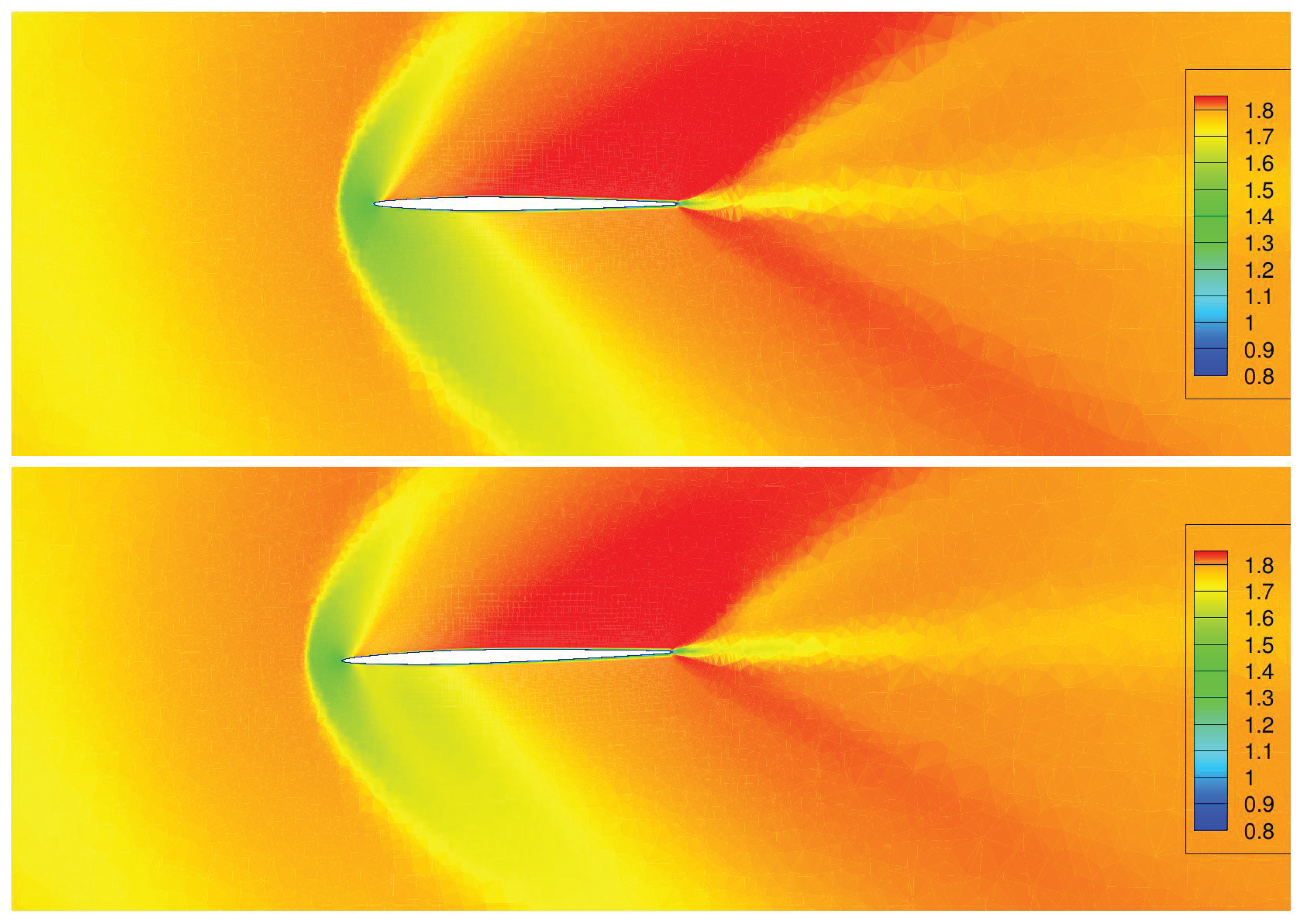
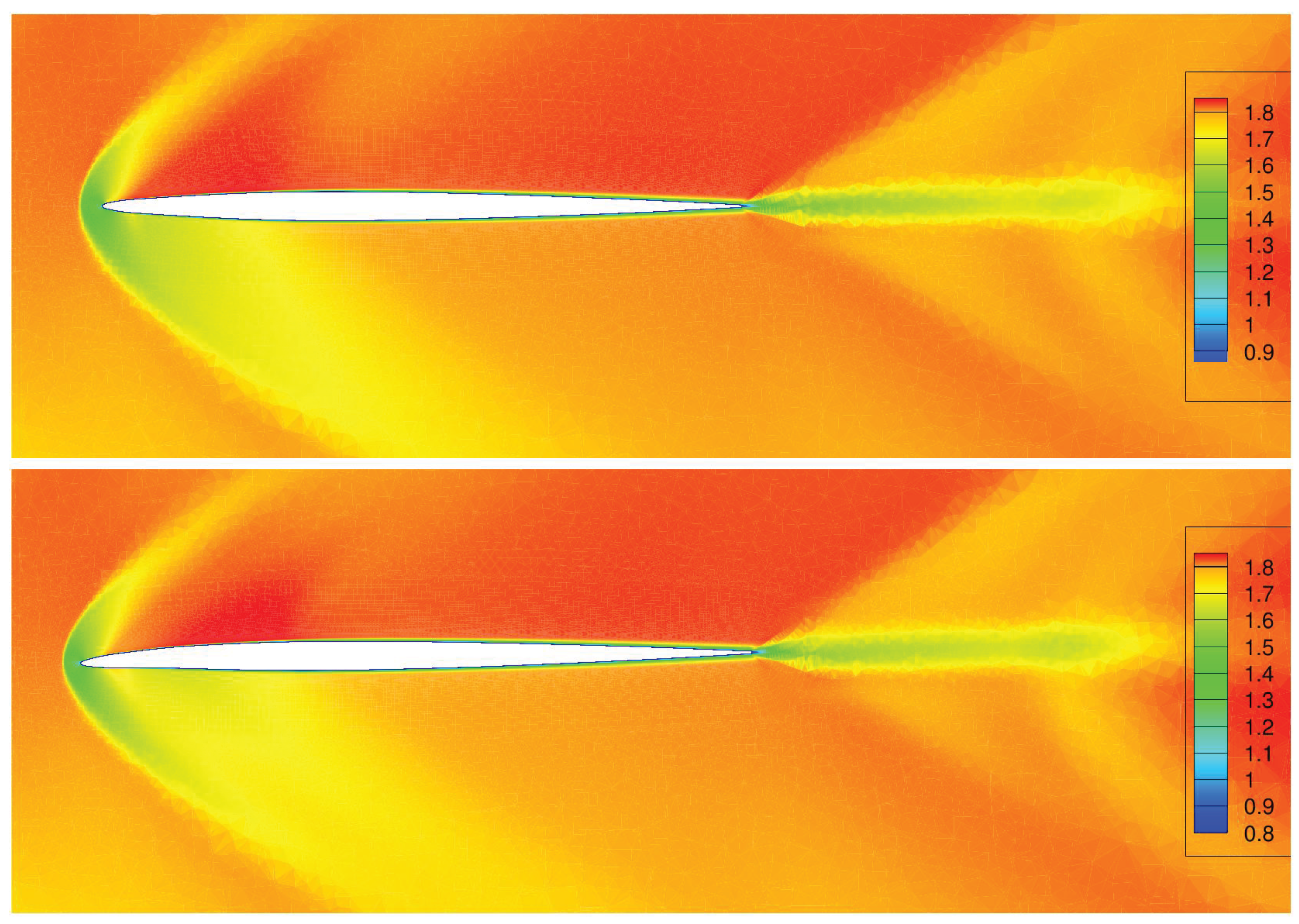
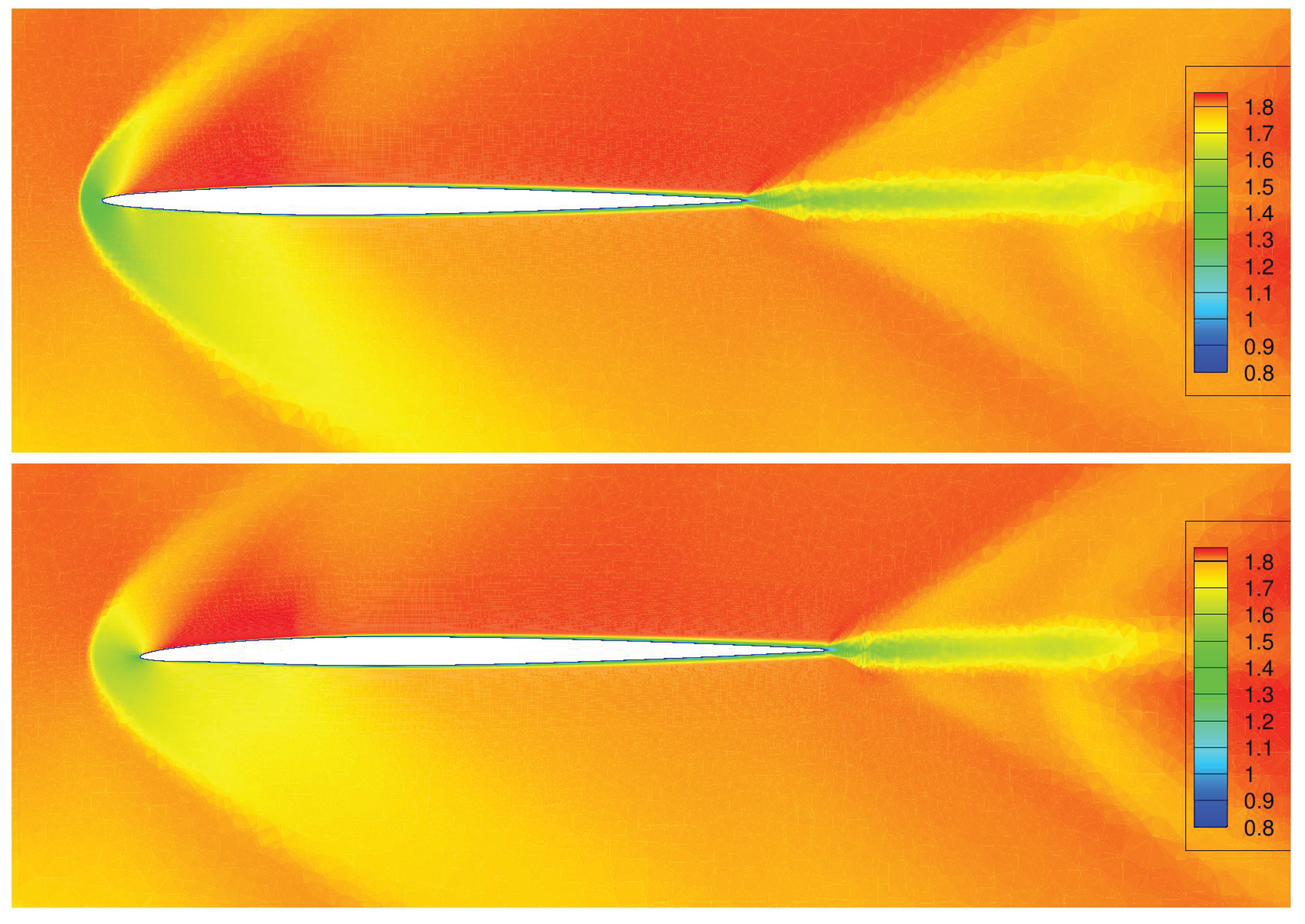
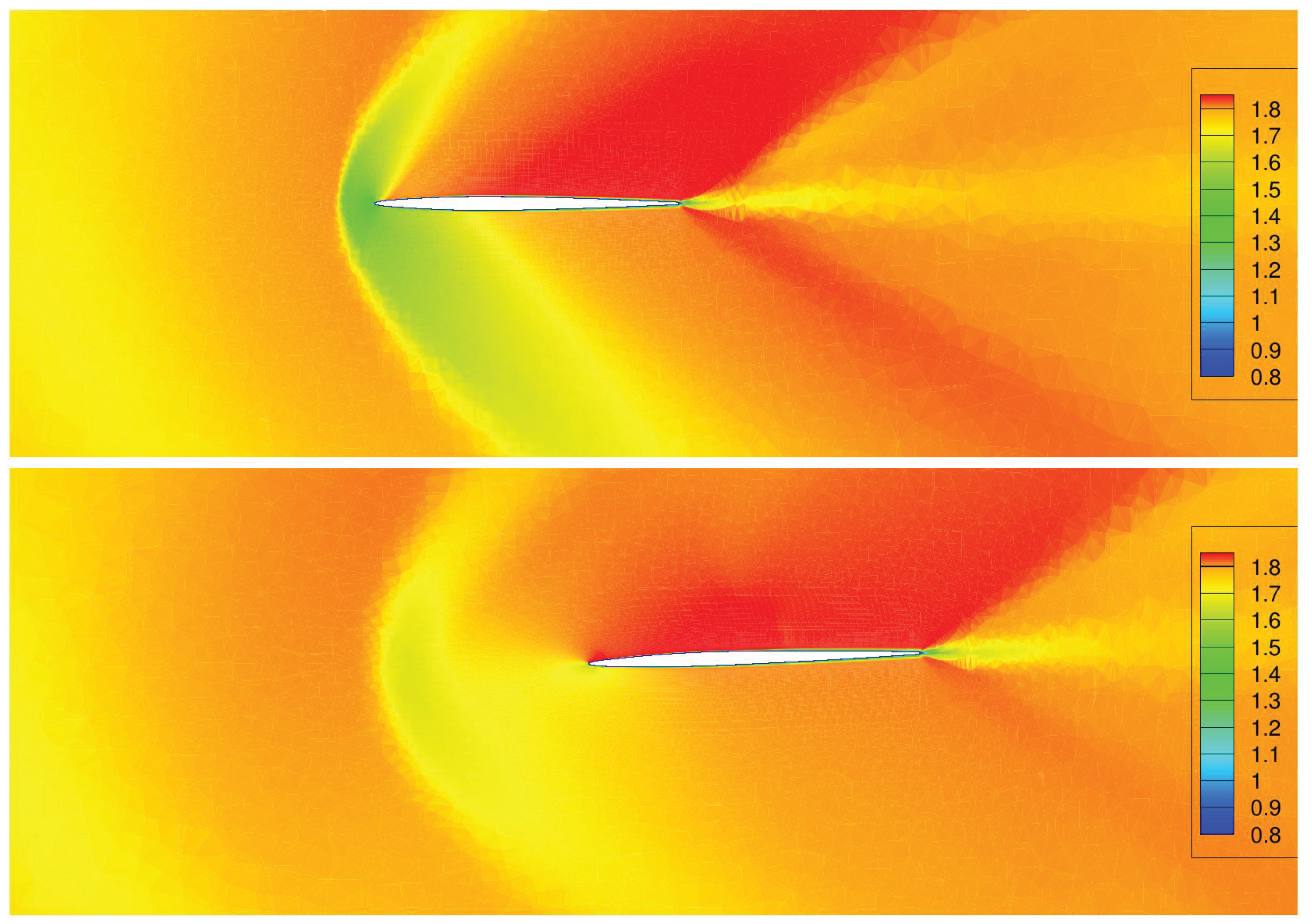
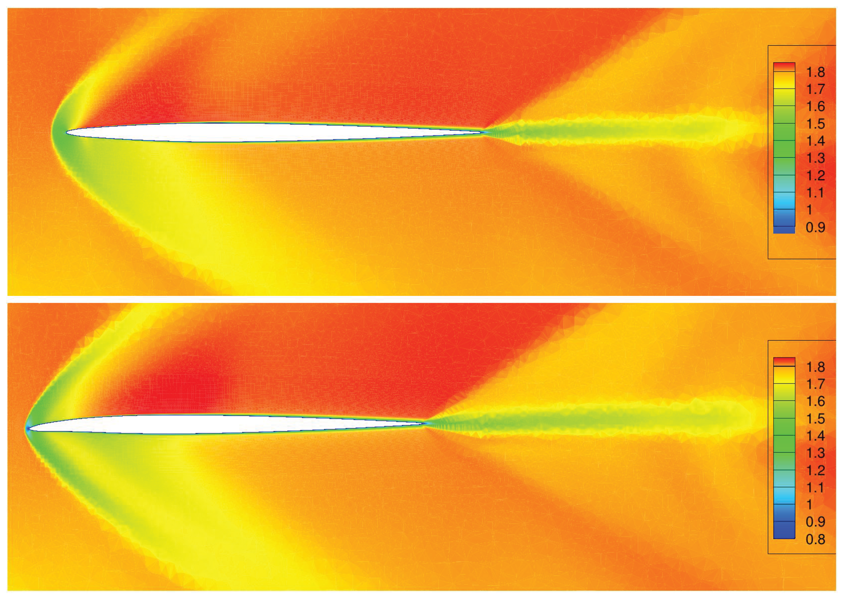
Figure 16 and Figure 17 show a comparison of the fields of local Mach number around the cross-section of the wing of the baseline (top) and the aerodynamic optimal shape (bottom) at

Y / b = 0.45

and

0.8

respectively. The decreasing strength of the bow shockwave can be clearly seen at both position.

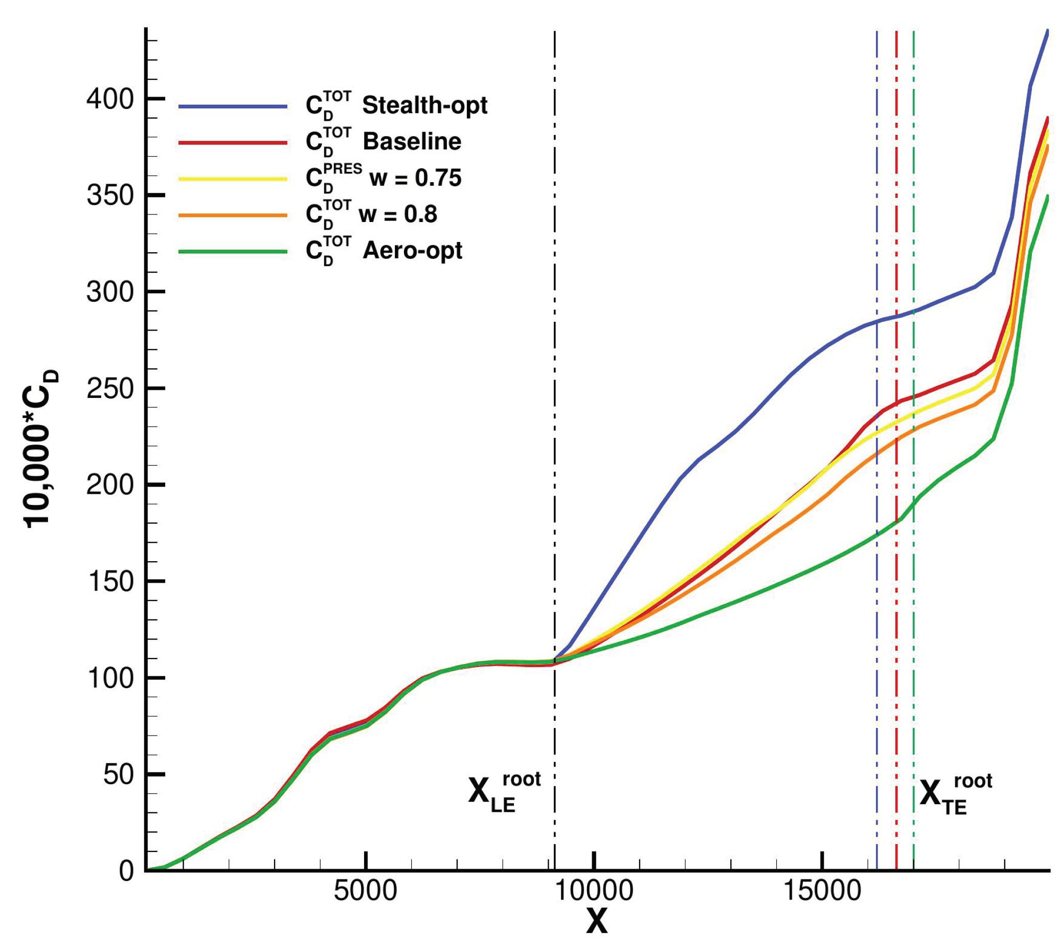
Figure 23 shows the integration of the total drag coefficients along the X axis for different shapes. The fuselage is unmodified by the optimization process so no difference can be seen for

X < X_{LE}^{root}

, but the drag of the aero optimal shape (red line) starts increasing later and more gradually than for the other shapes, which translates the gain in wave drag because of the higher leading sweep angles.

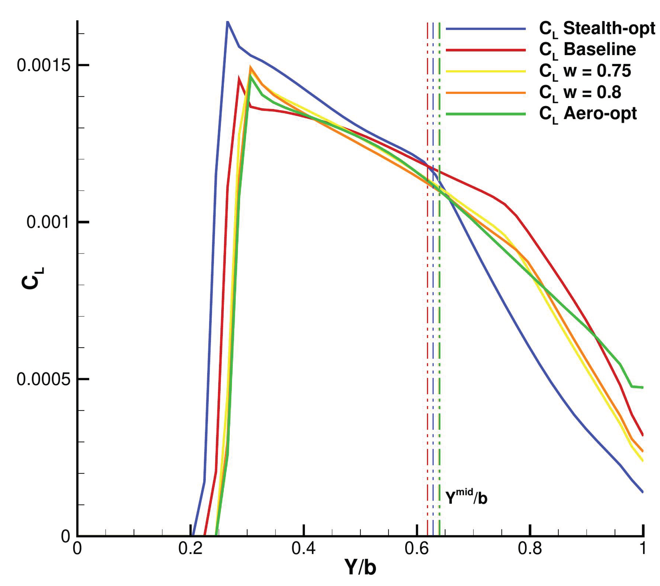
Figure 24 shows the distribution of the wing lift coefficient with respect to the normalized Y coordinate for different shapes. The lift is better distributed along the wing.

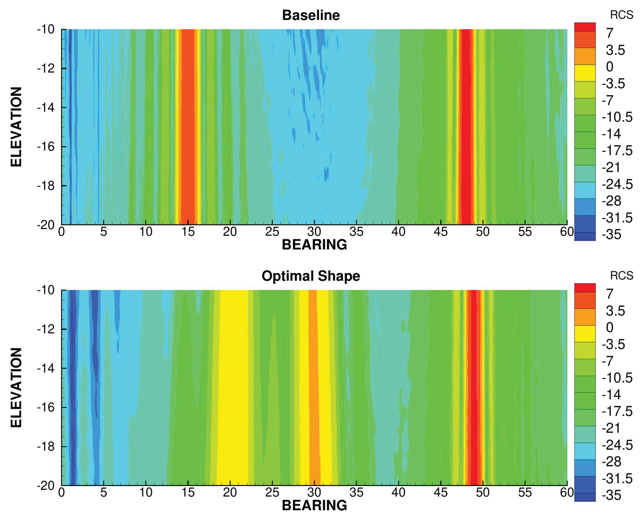
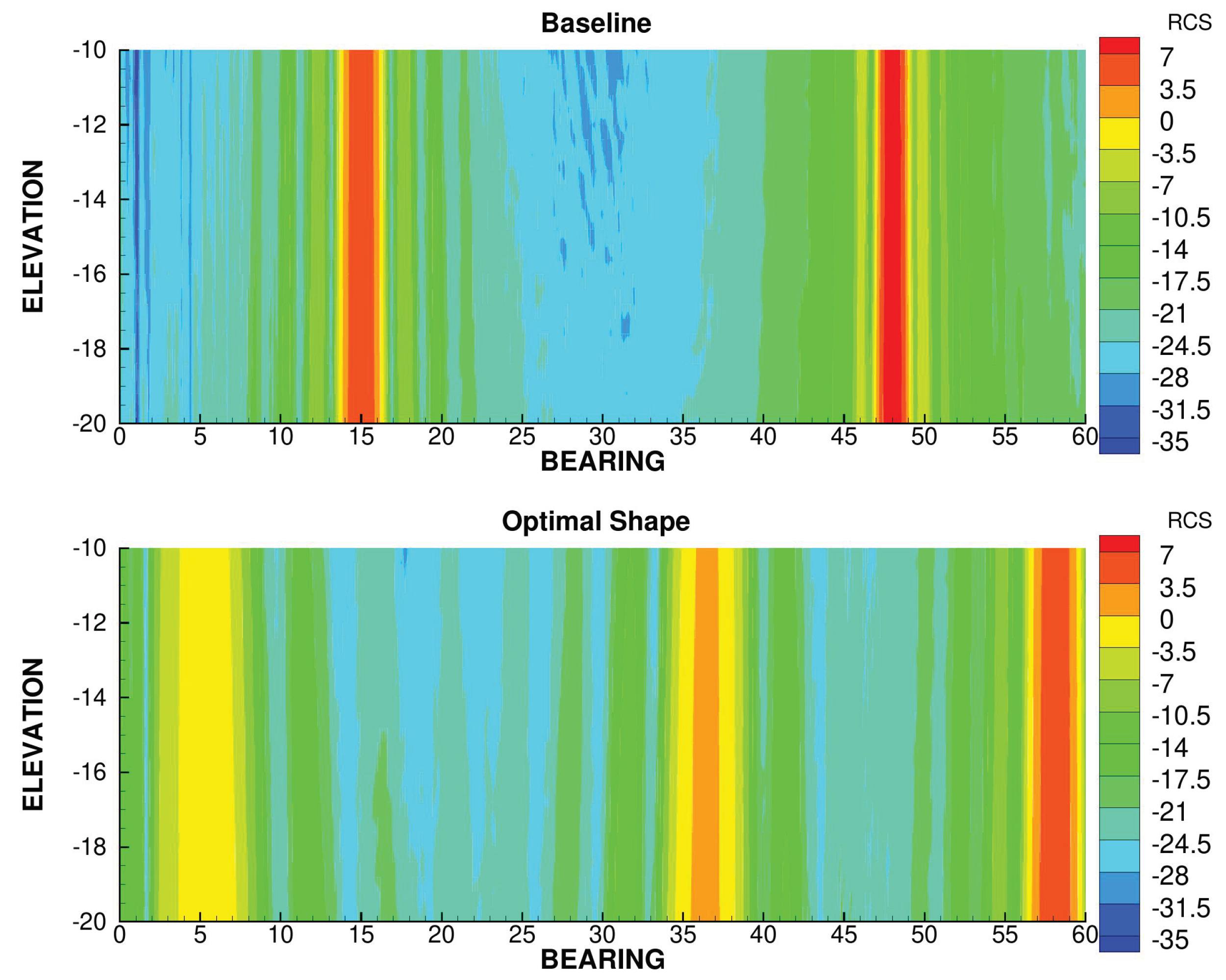
On the other hand, the multiple values of leading and trailing edge sweep angles has an adverse effect on the stealth criterion. This is because this leads to multiple RCS peaks as well as a wider spread of the RCS due to wedge diffraction, where the stealth criterion privileges a few, very sharp peaks.

In Figure 18, three peaks are visible. The very wide peak around 5

°

corresponds to the diffraction on the first section of the trailing edge wedge, and the peak around 36

°

corresponds to the second section of the trailing edge. The more intense peak around 58

°

corresponds to the specular reflection on the first section of the leading edge. The peak corresponding to the specular reflection on the second section of the leading would be in the 63

°

direction and is not visible on this figure.

7.2. Stealth Optimization

We then performed an optimization with a purely stealth cost function (

w = 0

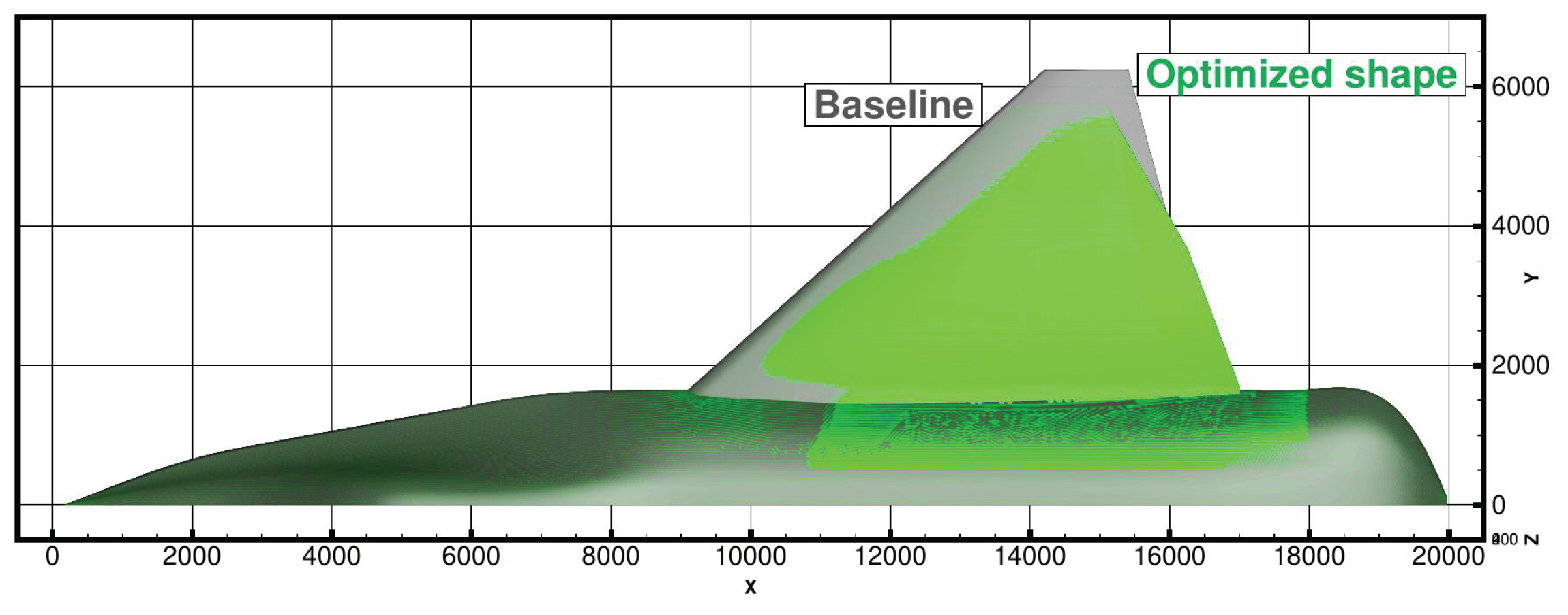
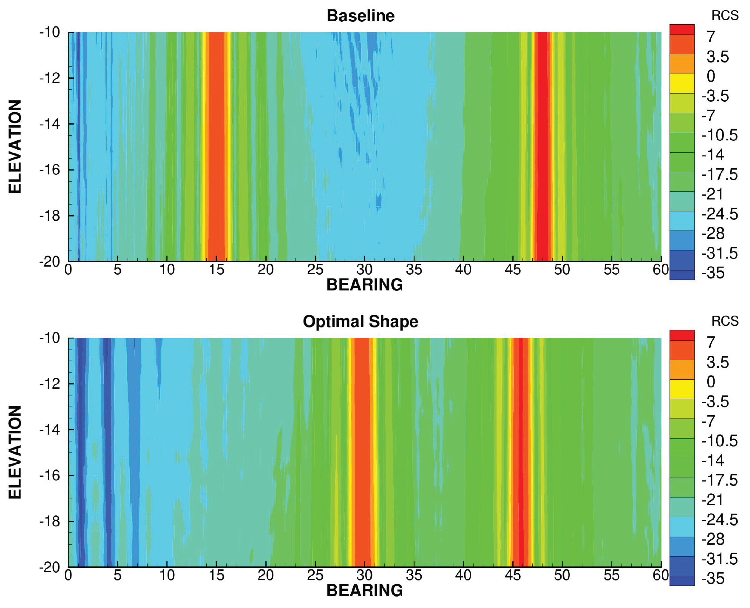
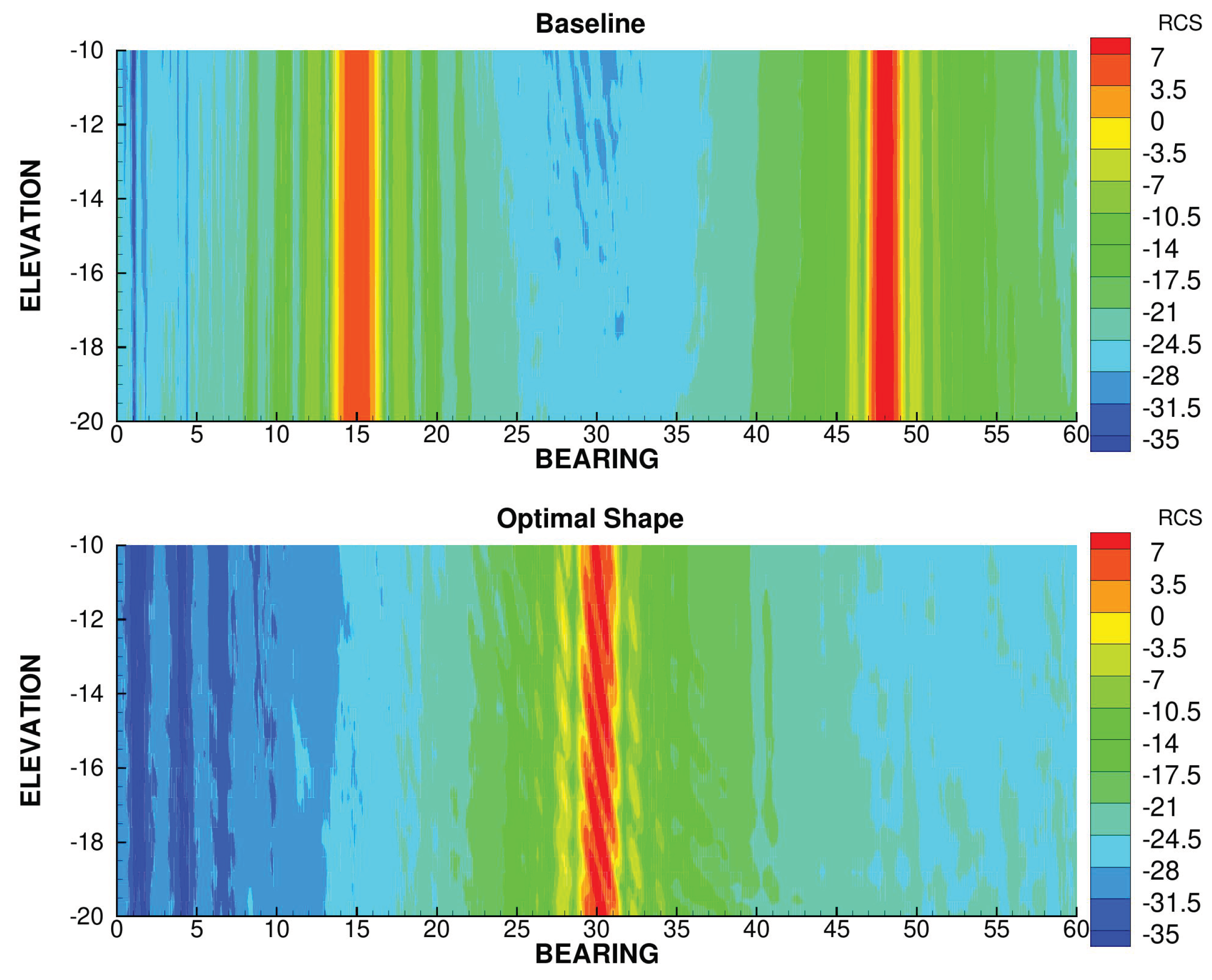
). The planform of the optimal shape compared to that of the baseline is presented of Figure 19. The leading and trailing edge are aligned with a sweep angle of

\pm 30^{°}

, which is the result expected from the choice of the stealth criterion. This allows the RCS to be concentrated in a sharp peak around a bearing angle of

30^{°}

, as seen in Figure 20.

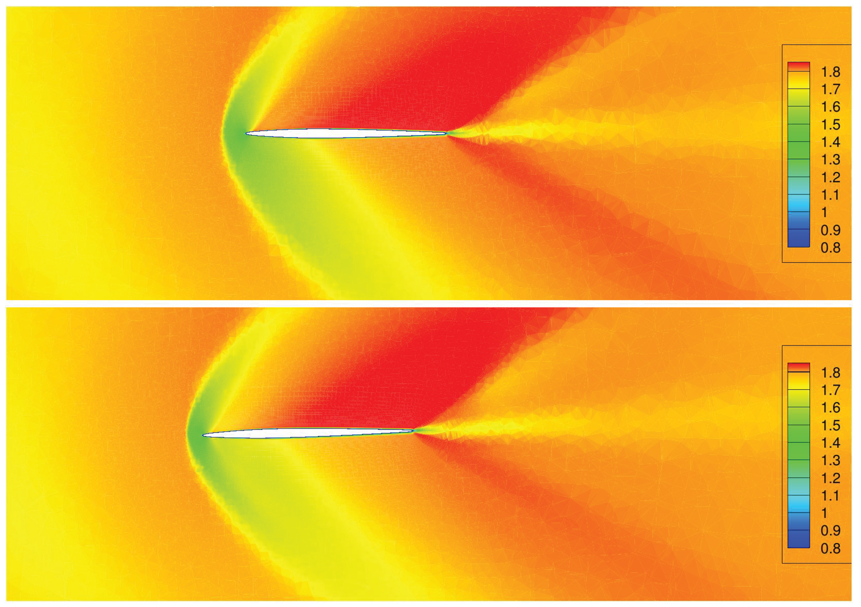
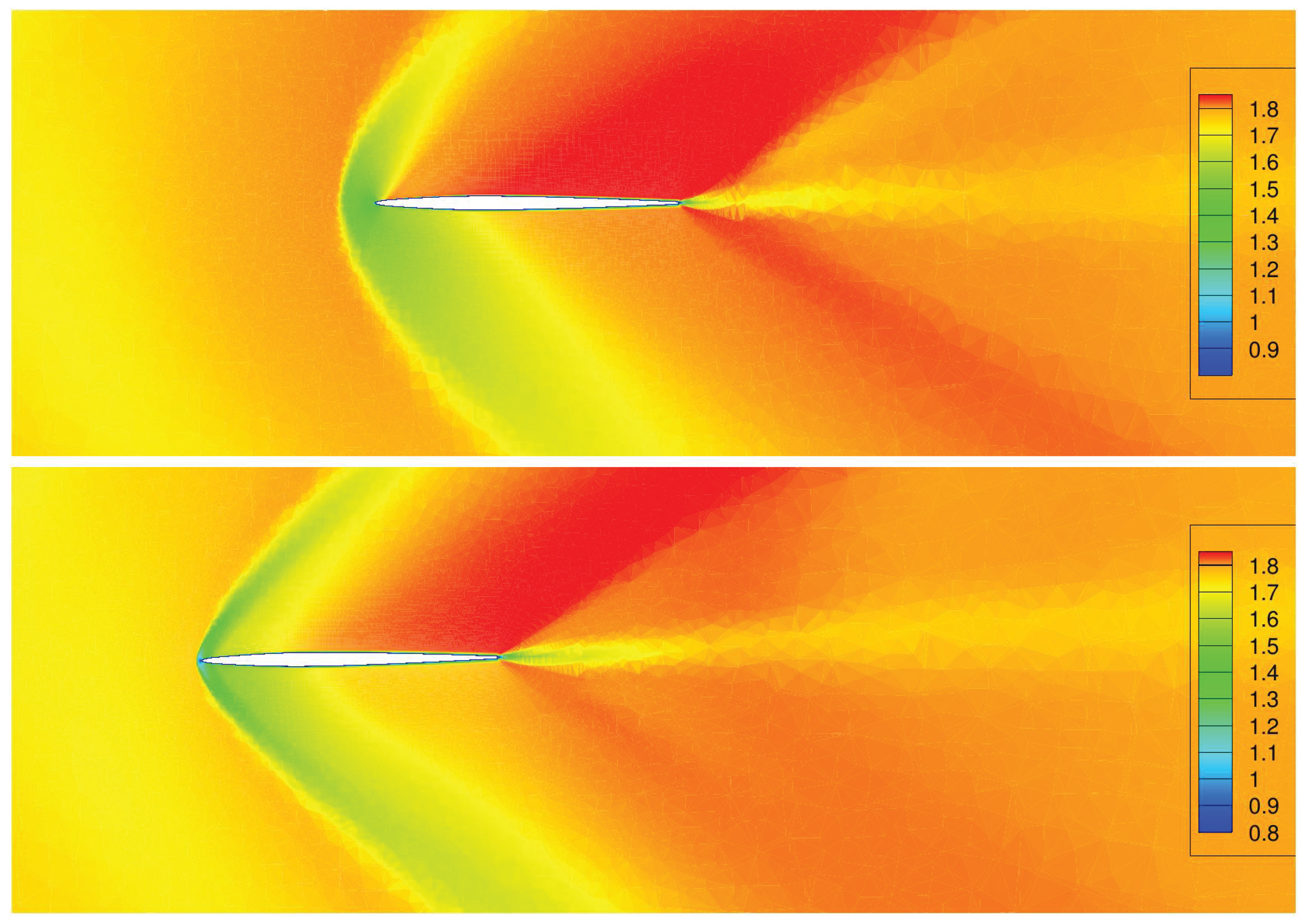
However, the decrease in leading edge sweep angle is very detrimental to the aerodynamic drag and particularly to the wave drag, as can be seen in Figure 21 and Figure 22, where a strong shock has appeared just upstream of the leading edge, which was absent from the other shapes. This is confirmed in Figure 23 which shows a much steeper and earlier increase in

C_{D}

than for the other shapes just downstream of the leading edge position. The pressure drag of the stealth-optimal shape alone is greater than the total drag on most of the baseline wing and on the totality of the aerodynamic optimal shape. The contribution of the pressure drag to the total drag is also much more important for the stealth optimal shape than the other shapes.

In Figure 24, we can see than the lift is more concentrated next to the root for the stealth-optimal shape than for the other shapes. On a realistic aircraft, such a behavior would be detrimental to stalling resistance at great AoA maneuvers for example.

Figure 23. Integration of C_D along the X axis.

Figure 24. Distribution of the wing C_L.

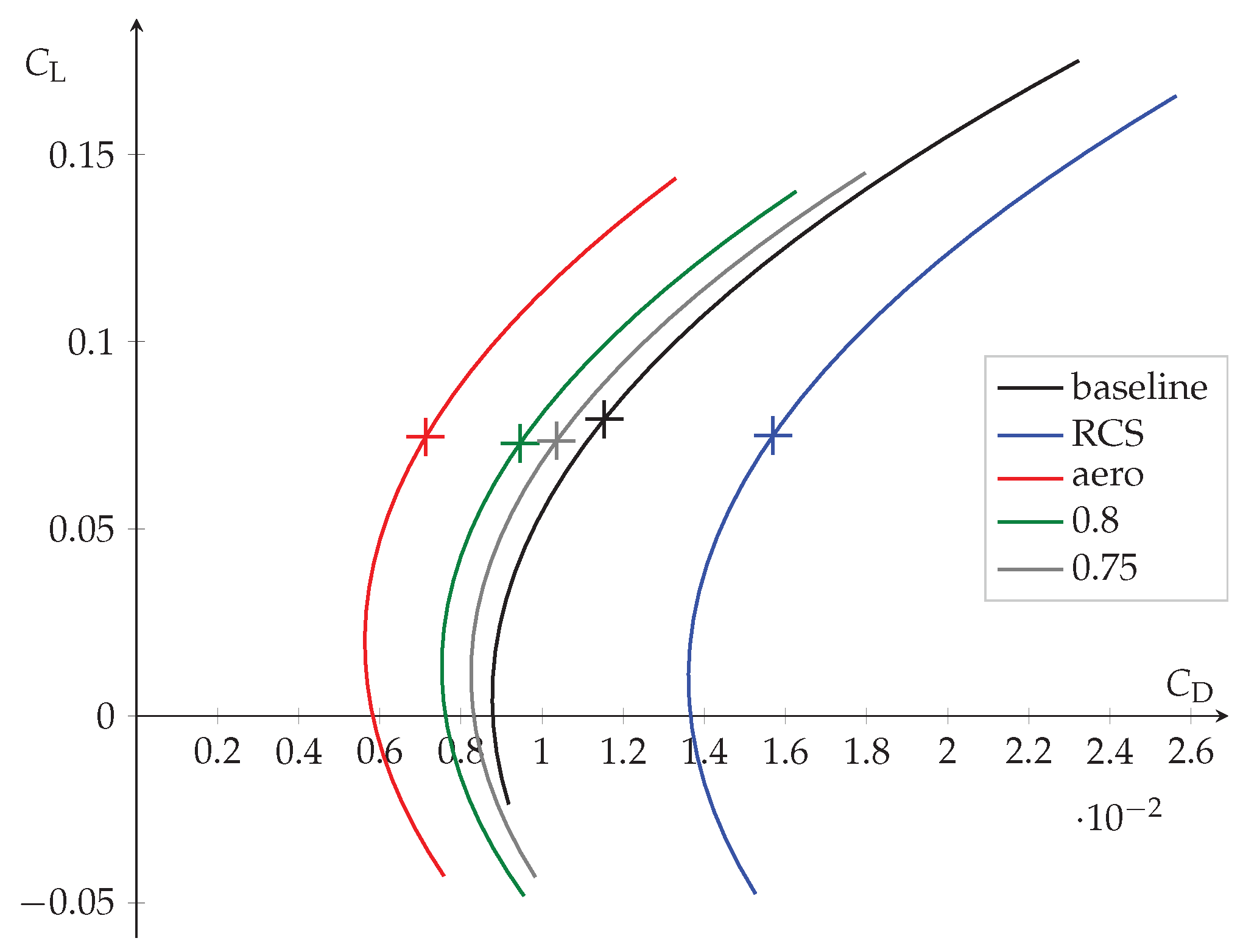
Figure 25. Comparison of the aerodynamic polars of the wings of the different shapes.

Table 2. Gradient-Based Method

7.3. Pareto Optimality

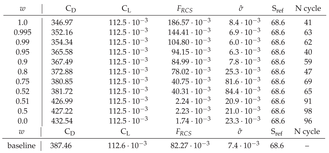
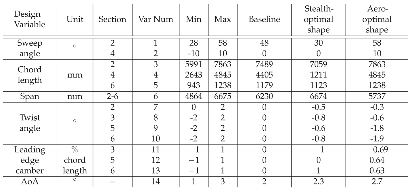
In the two previous section, we have shown that the requirements for a good aerodynamic shape and a good stealth shape are mainly in competition. Therefore, the need for compromise arise. We have explored different combination and drawn a Pareto front (Figure 34). We will present a few selected shapes. The values of the criteria and constraints for these shapes are summarized in Table 3.

Note that the Pareto front features three main attraction points, around

w = 0.9

w = 0.75

and

w \in [0, 0.5]

. Those attractors are probably due to the steepness of the weighting used in the RCS cost function (see Figure 12). The shapes around

w = 0.5

and below are essentially the same as the purely RCS optimal shape (Figure 19). The shape corresponding to

w = 0.75

and

w = 0.8

are showcased in Figure 27 and Figure 26 respectively. The drag difference between those shapes is pretty mild (8 drag count) and is largely due to the sweep angle as can be seen on the difference in pressure drag in Figure 23. The difference in RCS cost function is more notable. Though the RCS cost function is lower for the

w = 0.75

shape than the

w = 0.8

, its average RCS is higher. This is due to the secondary reflection peak at

20^{°}

aligning with the primary peak at

30^{°}

. Those two shapes are also better than the baseline both in terms of aerodynamic drag (7 and 15 drag counts lower than the baseline respectively) and RCS function, though the

w = 0.8

shape is barely better than the baseline.

Figure 26. Shape corresponding to the w = 0.8 point.

Figure 27. Shape corresponding to the w = 0.75 point.

Figure 28. Comparison of the distributions of local Mach number around the cross-section of the wing profile at Y/b = 0.45 between the baseline (top) and the w = 0.8 shape (bottom).

Figure 29. Comparison of the distributions of local Mach number around the cross-section of the wing profile at Y/b = 0.8 between the baseline (top) and the w = 0.8 shape (bottom).

Figure 30. omparison of the distributions of local Mach number around the cross-section of the wing profile at Y/b = 0.45 between the baseline (top) and the w = 0.75 shape (bottom).

Figure 31. Comparison of the distributions of local Mach number around the cross-section of the wing profile at Y/b = 0.8 between the baseline (top) and the w = 0.75 shape (bottom).

Figure 32. RCS of the w = 0.8 shape compared to that of the baseline.

Figure 33. RCS of the w = 0.75 shape compared to that of the baseline.

Figure 34. Pareto front

8. Conclusion

In this study, we presented a constrained, gradient-based aero-stealth optimization method in order to determine an optimal shape for an aircraft. For the sake of keeping computation time low, we showcased our method on a simplified shape with fifteen parameters, but it is able to deal with a more complex shape parametrized with hundreds of design variables.

We computed the aerodynamic gradient through an adjoint formulation and the RCS gradient with the help of the AD tool TAPENADE. We validated those gradients by comparing them to finite differences. The results show an acceptable difference.

After developing and validating the OP solver, we optimized a simplified aircraft geometry, with a weighted sum of the aerodynamic drag and a criterion based on the RCS repartition as the cost function. We varied the weights in order to identify a Pareto front. We extracted four of those optimal shapes and analyzed them.

The algorithm optimized the RCS mainly by tweaking the leading edge sweep angle and the chord length, which had an impact on the trailing edge sweep angle. This is because the stealth criterion depended heavily on the angular distribution of the RCS rather than merely its intensity.

When the weight is 1, the cost function is purely the aerodynamic drag. The optimal shape features a 40 drag count decrease, but at the cost of spreading the RCS across the observation window, which is detrimental to the stealth criterion. On the other hand, when the weight is 0, the cost function is purely the stealth criterion. The algorithm is able to improve the RCS of the shape across most of the observation window by concentrating the scattered wave in a single direction, but this has a dramatic impact on the wave drag of the aircraft.

With weights between 0.5 and 0.9, the optimizer was able to find trade-offs that were strictly better than the baseline shape.

Each optimization takes less than 100 cycles to reach an optimal solution, a cycle being the evaluation of either the cost function and the constraints or their gradients. This is efficient, and it allows optimizing more complex shapes or use higher fidelity methods while keeping a reasonable computation time.

Going forward, a more advanced method to identify the Pareto front, such as the one proposed by Desideri [30] would be beneficial.

Author Contributions

Conceptualization, Charles Thoulon, Gilbert Roge and Olivier Pironneau ; Methodology, Charles Thoulon and Gilbert Roge ; Software, Charles Thoulon ; Validation, Charles Thoulon ; Writing — original draft preparation, Charles Thoulon ; Writing — review, Gilbert Roge and Olivier Pironneau ; Supervision, Olivier Pironneau. All authors have read and agreed to the published version of the manuscript.

Funding

This research received no external funding

Acknowledgments:

Our thanks to Quentin Carayol, Hervé Steve and Nicolas Réau for their help to modify COPOLA, to Steven Kleinveld for his help with GANIMEDE and to Laurent Hascoët from INRIA for his help with TAPENADE. Finally, we are grateful to Sarah Julisson for maintaining and adapting the optimization system of Dassault-Aviation to our needs.

Conflicts of Interest

Authors Charles Thoulon and Gilbert Roge were employed by the company Dassault-Aviation. The remaining author declare that the research was conducted in the absence of any commercial or financial relationship that could be construed as a potential conflict of interest

References

Knott, E.F.; Schaeffer, J.F.; Tulley, M.T. Radar cross section; SciTech Publishing, 2004. [Google Scholar]
Aliaga, C.; Kopp, M.; Salui, K.B.; Mahapatra, D.; Sardesai, A. Aerodynamic and stealth studies of canard-wing Configurations at Transonic Speeds using Ansys Fluent & Ansys HFSS SBR+. AIAA AVIATION 2022 Forum, 2022, p. 3322. [CrossRef]
Lee, D.; Gonzalez, L.F.; Srinivas, K.; Auld, D.; Periaux, J. Multi-objective/multidisciplinary design optimisation of blended wing body UAV via advanced evolutionary algorithms. 45th AIAA Aerospace Sciences Meeting and Exhibit, 2007, p. 36. [CrossRef]
Wu, D.; Long, T.; Li, Y.; Jiang, M.; Huang, B. Aero-structure-stealth coupled optimization for high aspect ratio wing using adaptive metamodeling method. 15th AIAA/ISSMO Multidisciplinary Analysis and Optimization Conference, 2014, p. 2304. [CrossRef]
Jiang, X.; Zhao, Q.; Zhao, G.; Meng, C. Numerical Optimization on Aerodynamic/Stealth Characteristics of Airfoil Based on CFD/CEM Coupling Method. Transactions of Nanjing University of Aeronautics & Astronautics 2016, 33, 274–284. [Google Scholar]
Lyu, Z.; Xu, Z.; Martins, J. Benchmarking optimization algorithms for wing aerodynamic design optimization. Proceedings of the 8th International Conference on Computational Fluid Dynamics, Chengdu, Sichuan, China. Citeseer, 2014, Vol. 11, p. 585.
Martin, L. Conception aérodynamique robuste. PhD thesis, Université de Toulouse, Université Toulouse III-Paul Sabatier, 2010. [Google Scholar]
Hascoët, L.; Pascual, V. The Tapenade Automatic Differentiation tool: Principles, Model, and Specification. ACM Transactions On Mathematical Software 2013, 39. [Google Scholar] [CrossRef]
Lyu, Z.; Martins, J.R. Aerodynamic design optimization studies of a blended-wing-body aircraft. Journal of Aircraft 2014, 51, 1604–1617. [Google Scholar] [CrossRef]
Lyu, Z.; Kenway, G.K.; Martins, J.R. Aerodynamic shape optimization investigations of the common research model wing benchmark. AIAA journal 2015, 53, 968–985. [Google Scholar] [CrossRef]
Garnier, E.; Langlet, S.; Klotz, P.; Cadillon, J.; Simon, J.; Castelli, J.C.; Levadoux, D. Surrogate-based conception for aerodynamic/stealth compromise. AVT-324 Specialists’ Meeting on Multidisciplinary Design Approaches and Performance Assessment of Future Combat Aircraft, 2020.
Guerra, J. Optimisation multi-objectif sous incertitudes de phénomènes de thermique transitoire. PhD thesis, INSTITUT SUPERIEUR DE L’AERONAUTIQUE ET DE L’ESPACE (ISAE), 2016. [Google Scholar]
Liu, Z.; Song, W.; Han, Z.; Wang, Y. Multifidelity Aerodynamic/Stealth Design Optimization Method for Flying Wing Aircraft. ICAS 2021. [Google Scholar]
Zhou, Z.; Huang, J. Quantitative weight and two-particle search algorithm to optimize aero-stealth performance of a backward inclined vertical tail. Aerospace 2023, 10, 345. [Google Scholar] [CrossRef]
Pan, Y.; Huang, J.; Li, F.; Yan, C. Integrated design optimization of aerodynamic and stealthy performance for flying wing aircraft. Proceedings of the International MultiConference of Engineers and Computer Scientists 2017, 2, 15–17. [Google Scholar]
Li, M.; Bai, J.; Li, L.; Meng, X.; Liu, Q.; Chen, B. A gradient-based aero-stealth optimization design method for flying wing aircraft. Aerospace Science and Technology 2019, 92. [Google Scholar] [CrossRef]
Kleinveld, S.; Rogé, G.; Daumas, L.; Dinh, Q. Differentiated parametric CAD used within the context of automatic aerodynamic design optimization. 12th AIAA/ISSMO Multidisciplinary Analysis and Optimization Conference, 2008, p. 5952. [CrossRef]
Chalot, F. Industrial Aerodynamics. In Encyclopedia of Computational Mechanics; Fluids, chapter 12; Stein, E., de Borst, R., Hughes, T.J.R., Eds.; John Wiley & Sons, Ltd., 2004; Vol. 3. [Google Scholar]
Barclay, A. SQP methods for large-scale optimization; University of California: San Diego, 1999. [Google Scholar]
Laval, D. Application de méthodes asymptotiques à la simulation de la diffraction électromagnétique par un corps régulier. PhD thesis, Université Sciences et Technologies-Bordeaux I, 2006. [Google Scholar]
Stratton, J.A.; Chu, L. Diffraction theory of electromagnetic waves. Physical Review 1939, 56, 99. [Google Scholar] [CrossRef]
Michaeli, A. Elimination of infinities in equivalent edge currents, Part I: Fringe current components. IEEE Transactions on Antennas and Propagation 1986, 34, 912–918. [Google Scholar] [CrossRef]
Chalot, F.; Johan, Z.; Mallet, M.; Billard, F.; Martin, L.; Barré, S. Extension of methods based on the stabilized finite element formulation for the solution of the Navier–Stokes equations and application to aerodynamic design. Computer Methods in Applied Mechanics and Engineering 2023, 417, 116425. [Google Scholar] [CrossRef]
Alfonsi, G. Reynolds-averaged Navier–Stokes equations for turbulence modeling 2009.
Spalart, P.R.; Allmaras, S.R. One-equation turbulence model for aerodynamic flows. La Recherche Aerospatiale 1994, 1, 5–21. [Google Scholar]
Martin, L.; Roge, G. Calcul de la sensibilité d’ordre deux d’une observation aérodynamique. ESAIM: Proceedings. EDP Sciences 2009, 27, 138–155. [Google Scholar] [CrossRef]
Poggio, A.J.; Miller, E.K. Integral equation solutions of three-dimensional scattering problems; MB Assoc., 1970. [Google Scholar]
Carayol, Q. Développement et analyse d’une méthode multipôle multiniveau pour l’électromagnétisme. PhD thesis, Paris 6, 2002. [Google Scholar]
Jenn, D. Radar and laser cross section engineering; American Institute of Aeronautics and Astronautics, Inc., 2005. [Google Scholar]
Désidéri, J.A. MGDA Variants for Multi-Objective Optimization. 2012.

Figure 1. Flowchart of the automatic optimization process chain

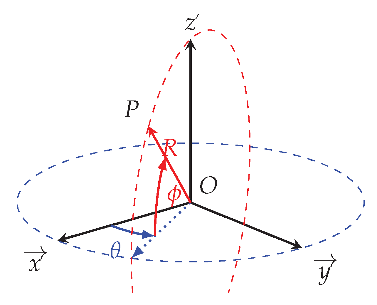
Figure 2. Definition of the bearing (θ) and elevation (ϕ) angles.

Figure 3. RCS of the sphere of radius R = 1m.

Figure 4. Comparison of the RCS function of the bearing angle predicted by COPOLA and BEM code on a GFA geometry (see Figure 5).

Figure 5. The Generic Fighter Aircraft.

Figure 6. Distribution of local Mach number around the fuselage of the GFA, in the symmetry plane.

Figure 7. istribution of local Mach number around the cross-section of the wing of the GFA, at Y/b = 0.45.

Figure 8. Distribution of local Mach number around the cross-section of the wing of the GFA, at Y/b = 0.8.

Figure 9. Profile of RCS with respect to the bearing angle on the GFA (elevation : ϕ = −20°).

Figure 10. The wing parametrized with the control sections and control points.

Figure 12. The function Γ_d(θ) with d = 30° for various values of τ.

Figure 13. Error between the gradient of the stealth cost function and the same computed by FD (both forward and central) function of the FD step size (ϵ).

Figure 14. Error between the gradient of the aerodynamic drag and the same computed by FD (both forward and centered) for the optimal step size determined for the CAD gradient.

Figure 15. Optimal shape from a purely aerodynamic standpoint.

Figure 16. Comparison of the distributions of local Mach number around the cross-section of the wing profile at Y/b = 0.45 between the baseline (top) and the aero-optimal shape (bottom).

Figure 17. Comparison of the distributions of local Mach number around the cross-section of the wing profile at Y/b = 0.8 between the baseline (top) and the aero-optimal shape (bottom).

Figure 18. RCS of the aero-optimal shape compared to that of the baseline.

Figure 19. Optimal shape from a purely low-observability standpoint.

Figure 20. RCS of the stealth-optimal shape compared to that of the baseline.

Figure 21. Comparison of the distributions of local Mach number around the cross-section of the wing profile at Y/b = 0.45 between the baseline (top) and the stealth-optimal shape (bottom).

Figure 22. Comparison of the distributions of local Mach number around the cross-section of the wing profile at Y/b = 0.8 between the baseline (top) and the stealth-optimal shape (bottom).

Table 1. Summary of the cost and contraints values for various shapes in the Pareto front.

Table 3. Summary of the values of the design variables for a few chosen optimal shapes.

Disclaimer/Publisher’s Note: The statements, opinions and data contained in all publications are solely those of the individual author(s) and contributor(s) and not of MDPI and/or the editor(s). MDPI and/or the editor(s) disclaim responsibility for any injury to people or property resulting from any ideas, methods, instructions or products referred to in the content.

© 2024 by the authors. Licensee MDPI, Basel, Switzerland. This article is an open access article distributed under the terms and conditions of the Creative Commons Attribution (CC BY) license (http://creativecommons.org/licenses/by/4.0/).

Copyright: This open access article is published under a Creative Commons CC BY 4.0 license, which permit the free download, distribution, and reuse, provided that the author and preprint are cited in any reuse.

MDPI Initiatives

Important Links

Choose an area of interest and we will send you notifications of new preprints at your preferred frequency.

Disclaimer

Gradient Based Aero-Stealth Optimization of a Simplified Aircraft

Abstract

1. Introduction

1.1. Gradient-Based Method

1.2. Aero-Stealth Optimization

1.3. Contribution

2. Methodology

2.1. The Physical Optics Approximation

2.2. Automatic Differentiation of Physical Optics

2.3. The aerodynamic solver

2.4. Adjoint Approach for CFD

2.4.1. Gradient with Respect to Aerodynamic Variables

2.4.2. Gradient with Respect to Geometric Variables

2.4.3. Summary

3. Validation

3.1. Validation of the COPOLA Code

4. Baseline Description

4.1. The CAD Modeler

4.2. Aerodynamic Analysis of the Baseline

4.3. Stealth Analysis of the Baseline

4.4. Optimization Parameters

5. Cost and Constraints

5.1. Aerodynamic Criterion

5.2. Stealth Criterion

5.3. Constraints

6. Sensitivity Validation

6.1. RCS with Respect to Geometric Variables

6.2. C D with Respect to Geometric and Aerodynamic Variables

7. Optimization Results

7.1. Aerodynamic Optimization

7.2. Stealth Optimization

7.3. Pareto Optimality

8. Conclusion

Author Contributions

Funding

Acknowledgments:

Conflicts of Interest

References

MDPI Initiatives

Important Links

Subscribe

6.2. $C_{D}$ with Respect to Geometric and Aerodynamic Variables