Submitted:
29 May 2024
Posted:
30 May 2024
You are already at the latest version
Abstract
Ranked Set Sampling (RSS) is a useful technique for improving the estimator of population mean when the sampling units in a study can be easily ranked than the actual measurement. RSS performs better than simple random sampling (SRS) when the mean of units corresponding to each rank is used. The performance of RSS can be increased further by assigning weights to the ranked observations. In this paper, we propose weighted RSS procedures to estimate the population mean of positively skew distributions. It is shown that the gain in the relative precisions of the population mean for chosen distributions are uniformly higher than those based on RSS. The gains in relative precisions are substantially high. Further, the relative precisions of our estimator are slightly higher than the ones based on Neyman’s optimal allocation model for small sample sizes. Moreover, it is shown that, the performance of the proposed estimator increases as the skewness increases by using the example of lognormal family of distributions.
Keywords:
rdered observations
; Neyman’s allocation
; Relative precision
; Skewness
; Unbiased estimator
; Weight
MSC: 62D05; 62G09; 94A20
1. Introduction
The Ranked Set Sampling (RSS) procedure has been used advantageously in agriculture, forestry, environmental, ecological and recently in human studies where the exact measurement of units is either difficult or expensive. For example, in forestry, the measurement of stem volume of standing trees is difficult but the ranking of the trees using their height and diameter at breast height is rather easy. For such situations, McIntyre (1952) introduced RSS to estimate the population mean. The RSS is a cost-efficient alternative to simple random sampling (SRS) if observations can be ranked according to the characteristic under investigation by means of visual inspection or other methods not requiring actual measurements. McIntyre (1952) indicated that the RSS procedure is superior to SRS procedure to estimate the population mean. However, Dell and Clutter (1972) and Takahasi and Wakimoto (1968) provided mathematical foundation for RSS. Dell and Clutter (1972) also showed that the estimator for population mean based on RSS is at least as efficient as the estimator based on SRS with the same number of measurements even though when there are ranking errors. Bhoj (2001) introduced RSS with unequal samples. Bhoj and Kushary (2016) proposed RSS with unequal samples for positively skew distributions with heavy right tails. RSS is a nonparametric procedure. However, recently, RSS has also been used in the parametric setup (see Bhoj and Ahsanullah (1996); Bhoj (1997a, 1997b); Lam et al. (1994); Stokes (1995).
The selection of ranked set sample of size k involves drawing k random samples with k units in each sample. The units in each sample are ranked by using judgment or other methods not requiring actual measurements. The unit with lowest rank is measured from the first sample, the unit with second lowest rank is measured from the second sample, and the procedure is continued until the unit with the highest rank is measured from the last sample. The k2 ordered observations in k samples can be displayed in the matrix form as:
We measure only k diagonal observations, and they constitute the RSS. We note that these k observations are independently but not identically distributed. In RSS, k is usually small to reduce the ranking errors and therefore, to increase the sample size, the above procedure is repeatedtimes to get the sample of size . In this paper, we assume m=1.
In the present paper, our main interest is to estimate the population mean for positively skew distributions with longer right tail. We propose estimators based on weighted ranked set sampling (WRSS) and compare their performance with the ones based on the usual RSS procedure and Neyman’s optimal allocation model. In section 2, we summarize the estimators of population mean based on RSS procedure and Neyman’s optimal solution. In section 3, we propose our WRSS procedure to estimate the population mean of skew distributions. First, we introduce WRSS procedure where we assign one low weight to the highest order statistics and calculated the relative precisions of the estimator based on WRSS, RSS and Neyman’s optimal procedure with respect to the estimator based on SRS. The procedures are used to obtain the relative precisions by using the four positively skew distributions. We also computed one set of weights for all four distributions for each k. In section 4, we derived optimal weights for the lowest and highest order statistics for the chosen distributions for each k. We then obtained one set of weights for the lowest and highest order statistics for each k which will maximize the sum of relative precisions of four distributions. In section 5, we generalize the use of all optimal weights for all order statistics for k=4 and k=5 for each distribution. We also obtained one set of weights for each k for the four chosen distributions. In section 6, to see the effect of increasing skewness, the relative precisions of estimators for lognormal family of distributions have been compared. In section 7, we summarize the results with recommendations.
2. Estimation of Mean
We consider first the usual RSS to estimate the population mean. Let denote the value of characteristic under study of order statistic. The mean and variance of the rank order statistic for set size k are denoted by and , respectively. We denote the population mean and variance by and , respectively. Then the unbiased estimator for based on RSS is given by
with the variance
The relative precision of compared to the estimator based on SRS with the same number of observations k (Bhoj and Chandra, 2019) is
where is the average within-rank variance.
For the skewed distribution, Neyman’s allocation provides the optimal allocation and the relative precision of the unbiased estimator of based on this model with respect of SRS with the same number of observations n and is given by (Bhoj and Chandra, 2019).
where, is the average within-rank standard deviation.
There are some unequal allocation models for the skew distributions in the literature (see, ‘t’ and ‘s, t’ model (Kaur et al., 1997); Systematic model (Tiwari and Chandra, 2011) and simple model (Chandra et al., 2018 and Bhoj and Chandra, 2019)). The Neyman’s allocation does not provide the integer values of which are necessary for any application. The procedure of making them integer is shown in Bhoj and Chandra (2019) and used in this paper. It is noted that the inequality always holds for the skew distributions.
3. WRSS with One Optimal Weight
In this section, we propose a weighted ranked set sampling (WRSS) with the optimal weight for the largest order statistic since the largest order statistic has the highest variance and higher bias of the estimator for the mean when we deal with the positively skew distributions. We define that the weights as,
The exact values of weights are proposed as follows:
Our weighted estimator for the population mean is
The relative precision of our biased estimator with respect to the estimator based on SRS is
The value of is to be chosen such that the is maximum. To find the optimum value of (for each k), the excel program of was developed and using the different iterations on , the values of was tested until it gets maximum. All the other values above and below from this optimal , starts decreasing.
We computed for all four chosen distributions lognormal (LN(0, 1)), Pareto (P(3.5) and P(4.5)) and Weibull (W(0.5)) and k=2(1)5. The values of , , and for these distributions and k=2(1)5 are presented in Table 1. The values of are much higher than , i.e., the relative precisions of the estimator based on RSS procedure. Furthermore, the are higher than , i.e., those based on Neyman’s optimal allocation model for all four distributions when . All relative precisions increase as k increases for LN(0,1), P(3.5) and P(4.5). However, for W(0.5), decreases as k increases. This may be because the distribution W(0.5) has extremely large skewness and kurtosis.
Now we attempt to compute one set of values of for four values of sample sizes, which will work well for all chosen four distributions. In these computations, was determined so that the sum of for the four distributions is close to the maximum. This optimum value of was found using the same iteration procedure in the developed excel program.
4. WRSS with Two Optimal Weights
In this Section, we propose a WRSS with two optimal weights for the two extreme order statistics. Here the weights for k>2 are defined as
The proposed exact weights are as follows:
where .
Our estimator of population mean is
The relative precision of with respect to the estimator based on SRS is
We calculate the optimal values of and using the iteration method. Based on these values, we computed along with and for chosen four distributions and sample sizes k=3, 4 and 5 are presented in Table 3. The gains in precisions of the estimator over are marginal. The gains of based on are substantially higher than the estimator based on RSS. is superior to the estimator based on Neyman’s optimal allocation model for all k for the LN(0,1) and P(3.5) distributions. The values of are higher than those of for the other two distributions for k=3 and 4. The gains of over for k=5 for these two distributions are marginal.
As we did in case of we attempt to compute one set of values of and for three values of sample sizes which will work well for all chosen four distributions. In these computations, and were determined so that the sum of relative precisions of for the four distributions is close to the maximum relative precision. The values of and , ,and for three sample sizes and four chosen distributions are presented in Table 4. The relative precisions of in Table 4 are higher than those of for each k in Table 2. The pattern of relative precisions are same as seen in Table 3.
5. WRSS with All Optimal Weights
Now, we extend WRSS with optimal weights for all order statistics for k=4 and 5. We take , and determine the optimal values of C and by minimizing MSE of the estimator by using , .
In the next step we use
The values of are chosen so that the value of is maximized. Then we repeat the procedure of computing the optimal values of C and with these new . The procedure is repeated until the value of achieves the maximum value. We did this by using the developed computer program in Excel.
The values of are presented in Table 5. We observe that the values of presented in Table 4 are higher than the values of based on one or two optimal weights which are given in Table 1 and Table 3.
As we did in section 3 and 4, we computed one set of values of C, and different fractions for k=4 and k=5 which work well for all chosen four distributions. In these computations, these values were determined so that the sum of for the four distributions is close to the maximum relative precision. These values along with ,and for k=4 and k=5 and four chosen distributions are presented in Table 6. As we expected the values of are smaller in Table 6 when compared to the values of in Table 5. However, the pattern of relative precisions remains the same.
6. WRSS with Increasing Skewness
In this section, we wish to study the performance of the three methods, RSS, WRSS and Neyman’s optimum allocation model with increasing values of skewness of a family of distributions. For this purpose, the lognormal distribution, has been considered. The pdf of is given by
Then skewness (Sk) and shape parameter (p) are given by
The performance of these three methods relative to SRS with k=4 is presented in Table 7 for lognormal family of distributions for a range of values of population standard deviation. The variances of the order statistics of the family of distributions were computed by using the variances of order statistics for different values of shape parameter (p) which are readily available in Balakrishnan and Chen (1999). From Table 7, we observe that as skewness increases the performance of (i) RSS method decreases, and (ii) Neyman’s and WRSS methods increases. The values of based on all and two optimal weights are higher than for all values of shape parameters, However, based on one optimal weight is higher than for all p>1.9. The rate of increase of relative precisions of the proposed estimators based on WRSS are more than that of estimator based on Neyman’s method (See Figure 1).
7. Conclusions and Discussion
In this paper, we proposed weighted ranked set sampling procedure to estimate the population mean of the distributions which are positively skew with heavy right tail. We chose four distributions: lognormal (LN(0, 1)), Pareto (P(3.5) and P(4.5)) and Weibull (W(0.5)). The means and variances of order statistics for these distributions are readily available in Harter and Balakrishnan (1996). We proposed three weighted ranked set sampling procedures. The first procedure is based on one optimal weight for the largest order statistics, the second procedure is to use the two optimal weights for the two extreme order statistics, and the third is the one which is based on k optimal weights. We calculated the relative precisions for each of these four distributions by using the WRSS procedure for each sample size. These relative precisions are much higher than the relative precisions of RSS estimator of mean. Furthermore, relative precisions of our estimators are higher than those which are based on Neyman’s optimal procedures for . The relative precisions of our estimator are even higher than Neyman’s procedure for k=5 for some distributions. Furthermore, we attempted to compute one set of weight(s) for each k for all the distributions and compared the relative precisions of our estimator with those of RSS and Neyman’s estimators. Although there is slight loss in the values of relative precisions, they are still higher than those of Neyman’s model for for all four distributions and either more than or very close to Neyman’s model for k=5. In general, as is expected, the relative precisions of our estimator based on all optimal weights are higher than the relative precisions of our estimator based on two and one optimal weight(s). The gain in relative precisions is however marginal.
We studied the performance of our proposed estimators for increasing skewness of a family of lognormal distributions. The relative precision of our estimator based on one optimal weight is higher than those of Neyman’s estimator when the shape parameter exceeds 1.9. The relative precisions of our estimator based on two and k optimal weights is uniformly higher than those of Neyman’s estimator for all values of shape parameter considered in Table 7. From Figure 1, we see that with the increasing values of skewness, the rate of increase of relative precisions of our proposed estimators based on WRSS are more than that of estimator based on Neyman’s method.
Based on the numerical computations of relative precisions, we recommend our estimator based on WRSS procedures for estimator of population mean of skew distributions with heavy right tail for small values of set sizes.
Conflict of Interest
There is no conflict of interest.
References
- Balakrishnan, N. and Chen, W. S. Handbook of Tables of order statistics from lognormal distribution with applications, Springer, U. S. A. 1999.
- Bhoj, D.S. New parametric ranked set sampling. Journal of Applied Statistical Sciences 1997, 6, 275-289.
- Bhoj, D.S. Estimation of parameters of extreme value distributions with ranked set samplingCommunication of Statistics: Theory and Methods 1997, 26(3), 653-667. [CrossRef]
- Bhoj, D. S. Ranked set sampling with unequal samples. Biometrics 2001, 57(3), 957-962. [CrossRef]
- Bhoj, D.S. and Ahsanullah, M. Estimation of the parameters of the generalized geometric distribution using ranked set sampling, Biometrics 1996, 52, 685-694. [CrossRef]
- Bhoj, D.S. and Chandra, G. Simple unequal allocation procedure for ranked set sampling with skew distributions. Journal of Modern Applied Statistical Methods 2019, 18(2), eP2811. [CrossRef]
- Bhoj, D.S. and Kushary, D. Ranked set sampling with unequal samples for skew distributions. Journal of Statistical computations and simulations 2016, 86(4), 676-681. [CrossRef]
- Chandra, G., Bhoj, D.S. and Pandey, R. Simple unbalanced ranked set sampling for mean estimation of response variable of developmental programs, Journal of Modern Applied Statistical Methods 2018, 17, 28. [CrossRef]
- Dell, T.R. and Clutter, J.L. Ranked set sampling theory with order statistics background. Biometrics, 1972, 28, 545–555. [CrossRef]
- Harter, H.L. and Balakrishnan, N. CRC handbook of tables for the use of order statistics in estimation, CRC Press, Boca Raton, New York, 1996.
- Kaur, A., Patil, G. P. and Taillie, C. Unequal allocation models for ranked set sampling with skew distributions. Biometrics 1997, 53, 123-130. [CrossRef]
- Lam, K., Sinha, B.K. and Wu, Z. Estimation of parameters of the two-parameter exponential distribution using ranked set sample. Annals of the Institute Statistical Mathematics 1994, 46, 723-736. [CrossRef]
- McIntyre, G. A. A method for unbiased selective sampling using ranked sets. Australian Journal of Agricultural Research 1952, 3, 385-390. [CrossRef]
- Stokes, S. L. Parametric ranked set sampling. Annals of the Institute of Statistical Mathematics 1952, 47, 465-482. [CrossRef]
- Takahasi, K. and Wakimoto, K. On unbiased estimates of the population mean based on the sample stratified by means of ordering. Annals of the Institute of Statistical Mathematics 1968, 20, 1-31.
- Tiwari, N. and Chandra, G. A systematic procedure for unequal allocation for skewed Distributions in Ranked Set Sampling. Journal of the Society of Agricultural Statistics 2011, 65(3), 331-338.
Figure 1.
Comparison of rate of relative precisions with increasing skewness.
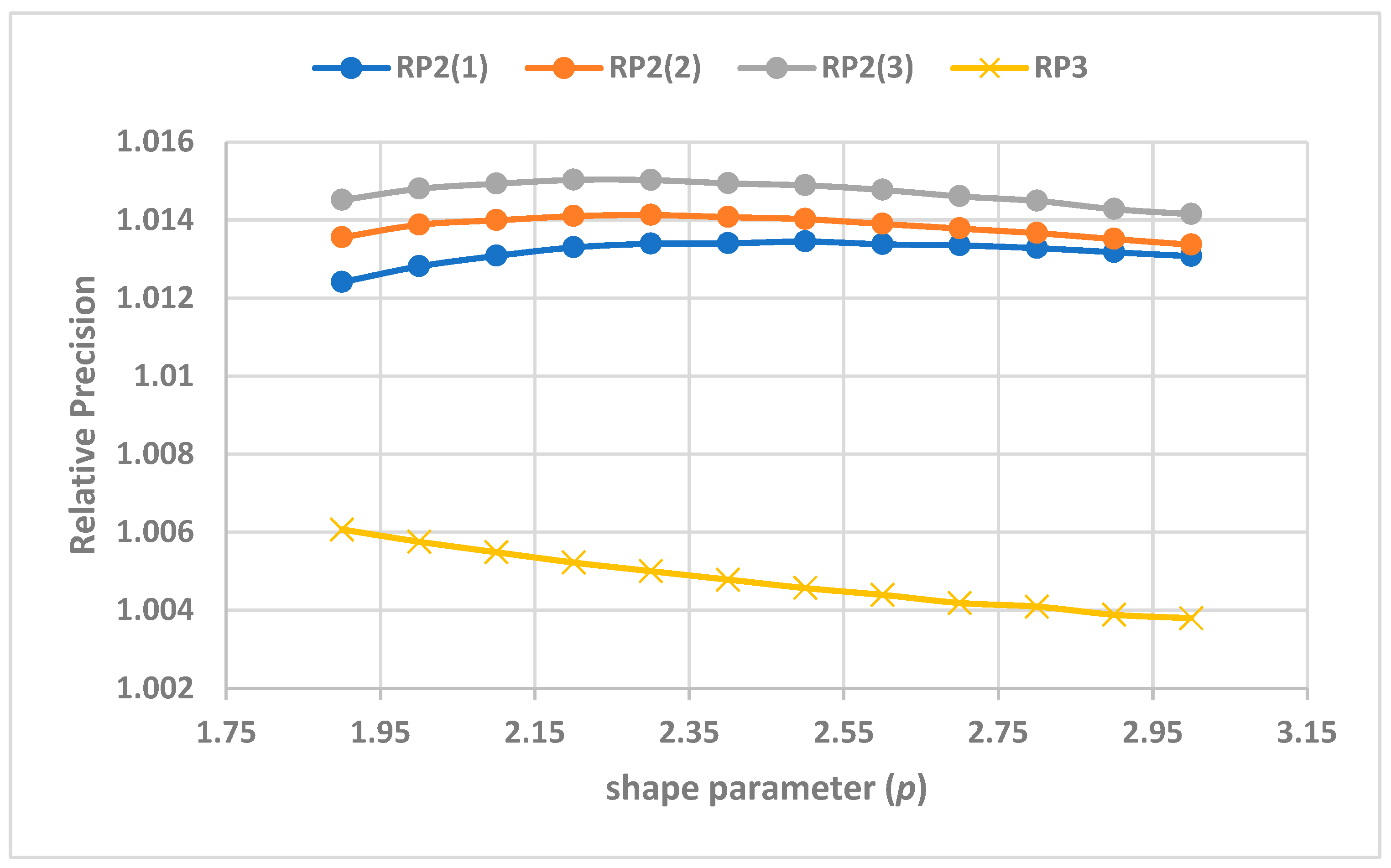

Table 1.
The RPs (, , ) at an individual optimal of each distribution for k = 2(1)5.
| Set size (k) | 2 | 3 | 4 | 5 | |
| LN(0,1) | 4.3798 | 3.2859 | 2.8028 | 2.5263 | |
| 1.1872 | 1.3393 | 1.4711 | 1.5891 | ||
| 2.5946 | 2.7278 | 2.8083 | 2.8845 | ||
| 1.5765 | 2.1182 | 2.6219 | 3.1347 | ||
| P(3.5) | 4.7900 | 3.5693 | 3.0417 | 2.7427 | |
| 1.1707 | 1.3073 | 1.4238 | 1.5269 | ||
| 2.7528 | 2.8579 | 2.9189 | 2.9805 | ||
| 1.5834 | 2.1273 | 2.6370 | 3.1434 | ||
| P(4.5) | 3.8151 | 2.8990 | 2.4962 | 2.2678 | |
| 1.2134 | 1.3901 | 1.5451 | 1.6847 | ||
| 2.3679 | 2.5338 | 2.6535 | 2.7676 | ||
| 1.5544 | 2.0810 | 2.5995 | 3.0878 | ||
| W(0.5) | 6.7391 | 4.4803 | 3.5837 | 3.0972 | |
| 1.1268 | 1.2362 | 1.3345 | 1.4250 | ||
| 3.6271 | 3.3698 | 3.2166 | 3.1379 | ||
| 1.6306 | 2.2105 | 2.7913 | 3.3840 | ||
Table 2.
The RP values (,, and total ) at combined optimal for k = 2(1)5.
| Set size (k) | 2 | 3 | 4 | 5 | |
| 5.0655 | 3.6004 | 2.9955 | 2.6618 | ||
| Total | 11.2063 | 11.3956 | 11.5215 | 11.7050 | |
| Total Maximum * | 11.3424 | 11.4893 | 11.5973 | 11.7705 | |
| LN(0,1) | 1.1872 | 1.3393 | 1.4711 | 1.5891 | |
| 2.5809 | 2.7207 | 2.8036 | 2.8811 | ||
| 1.5765 | 2.1182 | 2.6219 | 3.1347 | ||
| P(3.5) | 1.1707 | 1.3073 | 1.4238 | 1.5269 | |
| 2.7507 | 2.8578 | 2.9186 | 2.9794 | ||
| 1.5834 | 2.1273 | 2.6370 | 3.1434 | ||
| P(4.5) | 1.2134 | 1.3901 | 1.5451 | 1.6847 | |
| 2.3205 | 2.4963 | 2.6199 | 2.7363 | ||
| 1.5544 | 2.0810 | 2.5995 | 3.0878 | ||
| W(0.5) | 1.1268 | 1.23617 | 1.3345 | 1.4250 | |
| 3.5542 | 3.3208 | 3.1793 | 3.1082 | ||
| 1.6306 | 2.2105 | 2.7913 | 3.3840 | ||
*Total Maximum is the sum of of all the distributions at their respective optimum .
Table 3.
The RPs (, ) at individual optimal , of each distribution for k = 3(1)5.
| Set size (k) | 3 | 4 | 5 | |
| LN(0,1) | 3.3322 | 3.8383 | 4.3430 | |
| 1.0217 | 1.9580 | 6.9907 | ||
| 1.3393 | 1.4711 | 1.5891 | ||
| 2.7280 | 2.8982 | 3.1621 | ||
| 2.1182 | 2.6219 | 3.1347 | ||
| P(3.5) | 3.6003 | 4.1931 | 4.8037 | |
| 1.0134 | 2.0183 | 9.4583 | ||
| 1.3073 | 1.4238 | 1.5269 | ||
| 2.8579 | 3.0154 | 3.2847 | ||
| 2.1273 | 2.6370 | 3.1434 | ||
| P(4.5) | 2.8188 | 3.2036 | 3.6176 | |
| 0.9587 | 1.6485 | 3.9315 | ||
| 1.3901 | 1.5451 | 1.6847 | ||
| 2.5344 | 2.7072 | 2.9638 | ||
| 2.0810 | 2.5995 | 3.0878 | ||
| W(0.5) | 3.3947 | 3.7117 | 3.9996 | |
| 0.6463 | 1.0814 | 2.4127 | ||
| 1.2362 | 1.3345 | 1.4250 | ||
| 3.4286 | 3.2176 | 3.1936 | ||
| 2.2105 | 2.7913 | 3.3840 | ||
Table 4.
The RPs (,, and total ) at combined optimal , for k = 3(1)5.
| Set size (k) | 3 | 4 | 5 | |
| 3.4245 | 3.8499 | 4.2613 | ||
| 0.9241 | 1.7370 | 5.3284 | ||
| Total | 11.4036 | 11.7566 | 12.5655 | |
| Total Maximum * | 11.5489 | 11.8384 | 12.6042 | |
| LN(0,1) | 1.3393 | 1.4711 | 1.5891 | |
| 2.7169 | 2.8937 | 3.1605 | ||
| 2.1182 | 2.6219 | 3.1347 | ||
| P(3.5) | 1.3073 | 1.4238 | 1.5269 | |
| 2.8549 | 3.0112 | 3.2772 | ||
| 2.1273 | 2.6370 | 3.1434 | ||
| P(4.5) | 1.3901 | 1.5451 | 1.6847 | |
| 2.4947 | 2.6841 | 2.9504 | ||
| 2.0810 | 2.5995 | 3.0878 | ||
| W(0.5) | 1.2362 | 1.3345 | 1.4250 | |
| 3.3371 | 3.1677 | 3.1773 | ||
| 2.2105 | 2.7913 | 3.3840 | ||
*Total Maximum is the sum of of all the distributions at their respective and .
Table 5.
The RPs (,and ) at individual optimal C, and of each distribution for k = 4 and 5.
| LN(0,1) | P(3.5) | P(4.5) | W(0.5) | ||
| k=4 | 0.2136 | 0.2070 | 0.2693 | 0.2191 | |
| 0.0937 | 0.0870 | 0.1069 | 0.0830 | ||
| 0.5902 | 0.5827 | 0.5704 | 0.6484 | ||
| 0.4098 | 0.4173 | 0.4296 | 0.3516 | ||
| 1.4711 | 1.4238 | 1.5451 | 1.3345 | ||
| 2.9401 | 3.0510 | 2.7304 | 3.2862 | ||
| 2.6219 | 2.7913 | 2.6370 | 2.5995 | ||
| k=5 | 0.0827 | 0.0767 | 0.0905 | 0.0799 | |
| 0.0702 | 0.0648 | 0.0785 | 0.0686 | ||
| 0.3346 | 0.3260 | 0.3590 | 0.3491 | ||
| 0.4011 | 0.4013 | 0.3774 | 0.4143 | ||
| 0.2643 | 0.2727 | 0.2636 | 0.23660 | ||
| 1.5891 | 1.5269 | 1.6847 | 1.4250 | ||
| 3.2583 | 3.3652 | 3.0329 | 3.3215 | ||
| 3.1347 | 3.1434 | 3.0878 | 3.3840 | ||
Table 6.
The values of and total at combined optimal values of , and for k = 4 and 5.
| Set size | Total | Total Max * | |||||||||
| LN(0,1) | P(3.5) | P(4.5) | W(0.5) | ||||||||
| k=4 | 0.2210 | 0.0911 | 0.5967 | 0.4033 | 2.9367 | 3.0467 | 2.7018 | 3.2452 | |||
| k=5 | 0.0824 | 0.0700 | 0.3397 | 0.3992 | 0.2611 | 3.2577 | 3.3587 | 3.0164 | 3.3078 | 11.9303 | 12.0077 |
*Total Maximum is the sum of of all the distributions at their respective , and .
Table 7.
The values of , and for Lognormal distributions for k=4.
| p | for | For | For | ||||||||||
| C | |||||||||||||
| 1.8 | 3.40 | 2.07 | 2.715 | 1.633 | 0.301 | 0.124 | 0.556 | 0.444 | 1.702 | 2.490 | 2.552 | 2.568 | 2.520 |
| 1.9 | 3.70 | 2.16 | 2.848 | 1.674 | 0.289 | 0.119 | 0.561 | 0.439 | 1.665 | 2.521 | 2.587 | 2.606 | 2.535 |
| 2.0 | 4.00 | 2.24 | 2.978 | 1.714 | 0.279 | 0.115 | 0.565 | 0.435 | 1.632 | 2.553 | 2.623 | 2.644 | 2.550 |
| 2.1 | 4.30 | 2.33 | 3.105 | 1.753 | 0.268 | 0.112 | 0.569 | 0.431 | 1.603 | 2.587 | 2.660 | 2.684 | 2.564 |
| 2.2 | 4.60 | 2.41 | 3.229 | 1.790 | 0.258 | 0.108 | 0.573 | 0.427 | 1.576 | 2.621 | 2.697 | 2.724 | 2.577 |
| 2.3 | 4.90 | 2.48 | 3.351 | 1.825 | 0.249 | 0.105 | 0.577 | 0.424 | 1.552 | 2.656 | 2.735 | 2.765 | 2.590 |
| 2.4 | 5.21 | 2.56 | 3.471 | 1.859 | 0.240 | 0.102 | 0.580 | 0.420 | 1.530 | 2.692 | 2.774 | 2.806 | 2.603 |
| 2.5 | 5.51 | 2.64 | 3.588 | 1.891 | 0.231 | 0.099 | 0.583 | 0.417 | 1.510 | 2.728 | 2.813 | 2.848 | 2.615 |
| 2.6 | 5.82 | 2.71 | 3.704 | 1.923 | 0.223 | 0.097 | 0.587 | 0.413 | 1.491 | 2.765 | 2.852 | 2.890 | 2.626 |
| 2.7 | 6.13 | 2.79 | 3.818 | 1.953 | 0.215 | 0.094 | 0.590 | 0.410 | 1.474 | 2.802 | 2.891 | 2.932 | 2.637 |
| 2.8 | 6.44 | 2.86 | 3.930 | 1.981 | 0.207 | 0.092 | 0.593 | 0.407 | 1.458 | 2.839 | 2.931 | 2.975 | 2.648 |
| 2.9 | 6.75 | 2.94 | 4.040 | 2.009 | 0.200 | 0.090 | 0.595 | 0.405 | 1.444 | 2.876 | 2.970 | 3.017 | 2.658 |
| 3.0 | 7.07 | 3.01 | 4.149 | 2.035 | 0.193 | 0.088 | 0.598 | 0.402 | 1.430 | 2.914 | 3.010 | 3.060 | 2.668 |
Note: Here represents the proposed estimator based on all optimal weights and are the based on one, two and all optimal weights, respectively.
Disclaimer/Publisher’s Note: The statements, opinions and data contained in all publications are solely those of the individual author(s) and contributor(s) and not of MDPI and/or the editor(s). MDPI and/or the editor(s) disclaim responsibility for any injury to people or property resulting from any ideas, methods, instructions or products referred to in the content. |
© 2024 by the authors. Licensee MDPI, Basel, Switzerland. This article is an open access article distributed under the terms and conditions of the Creative Commons Attribution (CC BY) license (http://creativecommons.org/licenses/by/4.0/).
Copyright: This open access article is published under a Creative Commons CC BY 4.0 license, which permit the free download, distribution, and reuse, provided that the author and preprint are cited in any reuse.


