1. Introduction
The rapid urbanization in China has led to notable alterations in both urban and rural spatial structures, marked expansion of construction land, and the gradual depletion of surrounding natural resources such as cropland, woodland, grassland, and wetlands (López et al., 2001; Mao et al., 2018; Van Vliet, 2019). This phenomenon has resulted in various environmental issues (Bhatta, 2010).The mountainous areas of southwest China are characterized by high forest coverage and rich biodiversity (Qian et al., 2020), eroded by urban sprawl, fragmented rural settlements and agroforestry patches that themselves are affected by mountain topography and distribution systems (Tan et al., 2006), after urban construction and expansion, it becomes more fragmented by roads, public services, buildings and so on, and gradually suffers erosion (Su et al., 2014). However, these small and fragmented patches of agriculture and forestry do highlight the characteristics of mountainous regions, because of their complex terrain, it is difficult to scale single crop cultivation like plain areas, and because of their unique mountain environmental characteristics, local supplies of wild food and medicinal plants (Abdullah et al., 2021; Farina, 2000; Halada et al., 2011) , habitat maintenance and biodiversity conservation (Körner, 2004) , hand-planted cultural preservation (Xu et al., 2005) , urban green infrastructure (Sanesi et al., 2017) , therefore, small-scale agroforestry patches (Later referred to as SAP) can be of great concern in Europe (Plieninger and Bieling, 2013) .
In land use of China, SAP are small-scale and scattered agricultural and forestry land, which are not included in the protection zone. According to China’s national and local laws and policies, the occupation of arable land, garden land and Woodland of less than 3.3 hectare is not strictly controlled by law, only more than 3.3 hectares of agricultural and forestry land are subject to specific regulatory requirements (Chongqing municipality stipulates that more than 3.3 hectares of Cultivated land and garden land will be treated as high-standard cultivated land, while Cultivated land and garden land below this area, although still can not be occupied, has strict protection rules and is difficult to be occupied), however, this part of agricultural and forestry land is easy to be swallowed up by construction land in the area of urban planning/impact area, and the impact outside the urban planning area is relatively small. The definition of fragmented agroforestry land in this paper refers to the portion below 3.3. This part of the agricultural and forestry land in the mountain environment, the total area of the agricultural and forestry land will not be less than 3.3 hectares, the value of its comprehensive services is extremely significant, without a protection umbrella, they are extremely vulnerable to erosion. Hence, investigating the conservation and utilization of agricultural and forestry lands is of paramount importance. The protection and utilization of Small Agricultural and Forestry Patches (SAP) in mountainous cities are particularly significant as they contribute to essential ecological processes.
To prevent further degradation due to urban expansion and effectively safeguard small agricultural and forest patches, understanding the transformation dynamics of Small Agricultural and Forestry Patches (SAP) along the urban-rural gradient is crucial for devising scientifically sound protection and planning strategies. The concept of the Urban-to-Rural Gradient, introduced by McDonnel, examines the ecological processes in complex urban-rural spatial environments and the impact of urbanization on such spaces. McDonnel extensively investigated urban-rural gradients from downtown New York to rural Litchfield County, Connecticut (along a 140 × 20 km research transect), unveiling the characteristics and causes of forest ecosystem structure, soil composition, climate, impermeability, land cover, and cultural composition along the gradient. This research aimed to develop a rational conservation strategy for natural resources along this trajectory (McDonnell et al., 2008). Additionally, various studies have explored woodlands (Burton et al., 2005; Carreiro and Tripler, 2005), cultivated land (Li et al., 2015), insects (Niemelä et al., 2002), birds (Clergeau et al., 1998; Garaffa et al., 2009), changes in heat island intensity (Yang et al., 2022), water quality transformation (Wear et al., 1998), and landscape index transformation (Kaminski et al., 2021) based on urban-rural gradients. Analyzing the changing characteristics of each factor along the urban-rural gradient provides a scientific foundation for planning and adaptive strategies.
Therefore, based on the urban-rural gradients, the study of small agricultural and forest patches in mountain cities is also applicable, and some studies have been done to divide the urban-rural gradients by the landscape index, the landscape characteristics of different gradient spaces (Kaminski et al. , 2021) , Land Use Change Trends (Cifaldi et al. , 2004) and biodiversity status (Walz, 2011) are described, any spatial and temporal changes in landscape structure affect processes of energy and material flow, ecological stability and other properties and characteristics (Tlapáková et al. , 2013) . Similarly, the transformation of SAP can also be described based on the calculation of Landscape Index. At present, there are various types of landscape indices (Cardille and Turner, 2017) , and there are many different choices of landscape indices that can reflect the transformation characteristics of SAP in mountain regions, the transformation characteristics of SAP are usually discussed in terms of its scale change, fragmentation and dispersion, connectivity, shape complexity, proportion of dominant landscape, etc. , the landscape indices included Patch area (PA), Patch density (PD), Edge density (ED), Dispersion index (DI), Landscape separation index (LSI), Landscape connectivity index (LCI), Aggregation Index (AI), Fractal dimension (FD) and Largest patch index (LPI)(Li and Reynolds, 1994) , to reflect their existence and changing characteristics.
Furthermore, there is a need for a more comprehensive understanding of the specific factors influencing the transformation of Small Agricultural and Forestry Patches (SAP), providing a foundation for tailoring specific control measures for SAP in distinct regions. It is widely acknowledged that the transformation is influenced by a combination of natural and artificial factors (Forman, 1995), encompassing natural disturbances such as landforms, hurricanes, and geological disasters (Lin et al., 2006), and human factors, including aspects of the urbanization process such as construction intensity, road size and density, and economic activities (UUEMAA et al., 2009; Yang and Liu, 2005). A thorough comprehension of the impact of these drivers on SAP is essential for formulating differentiated and targeted management rules for various SAP segments.
To sum up, this paper includes three research objectives:
1) landscape pattern transformation characteristics of SAP on urban-rural gradient in mountainous urban planning area?
2) the transformation characteristics of small-scale agroforestry elements (Cultivated land, garden land, woodland) on the urban-rural gradient in mountain urban planning area?
3) the relationship between geomorphologic and human factors and SAP and factor transformation?
2. Materials and Methods
2.1. Study Area
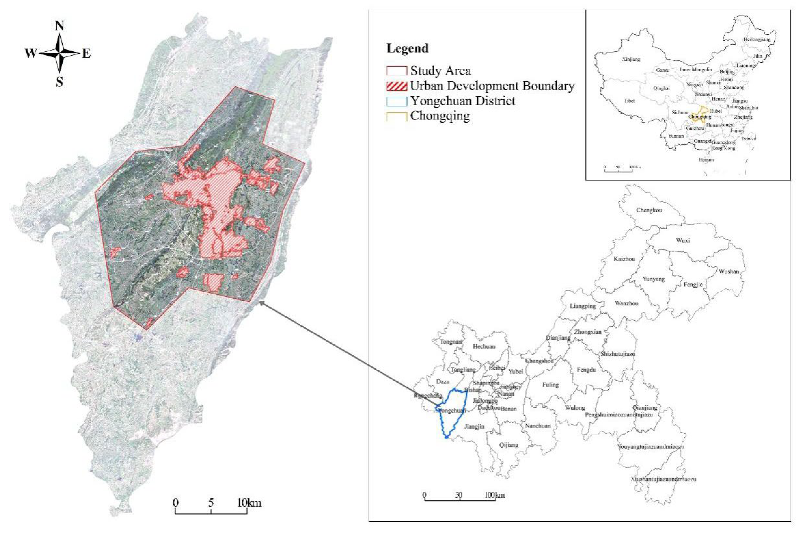
For the present case study, we selected Yongchuan District in Chongqing City, located in Southwest China. Chongqing stands out as one of the most developed cities in China, serving as a core city within the Cheng-Yu economic circle. Characterized by diverse topography and challenging landforms, Chongqing is a representative mountainous city, posing difficulties in construction (Huang, 2005). By visiting the districts of Chongqing, it is found that there are a lot of SAP existing in the urban planning area, which form the special landscape features of mountainous areas and are the potential resource elements of mountainous areas, as a part of urban and rural green infrastructure, it can play a social, economic, ecological and other composite functions. These fragmented agricultural and forestry lands show different morphological characteristics along the urban-rural gradients, especially in the area of urban planning area/affected area, and these SAP will gradually disappear as the city expands, planning areas are therefore considered as study areas. This selection of Chongqing Yongchuan Urban Planning Area (
Figure 1), an area of 175 square kilometers.
2.2. Research Framework
The study is divided into four steps: first, through the introduction part of the status of Agriculture and forestry in the Southwest Mountain region of policy analysis, select 3.3 hectares of unprotected agricultural and forestry land. Secondly, the samples were randomly selected from four different directions from rural to urban center, and divided into equal-distance grid of sample points. Thirdly, through the analysis of the data, the agricultural and forest patch and each element landscape index were calculated by Fragstats4.3. At the same time, the gradient change of the related factors was calculated, SPSS Spearman correlation analysis was used to study the relationship between small-scale agroforestry patch and its influencing factors, and to determine which factors are the main driving forces to promote the segmentation, fragmentation and even disappearance of agroforestry patch. Through the above research process, on the one hand, we can grasp the change characteristics of small-scale agricultural and forest patches, and provide scientific basis for the protection and utilization of small-scale agricultural and forest patches in urban planning area, on the other hand, we know the factors that affect the characteristics of the patch pattern, which can provide the basis for the management and control of the small-scale patch.
2.3. Study Object Selection
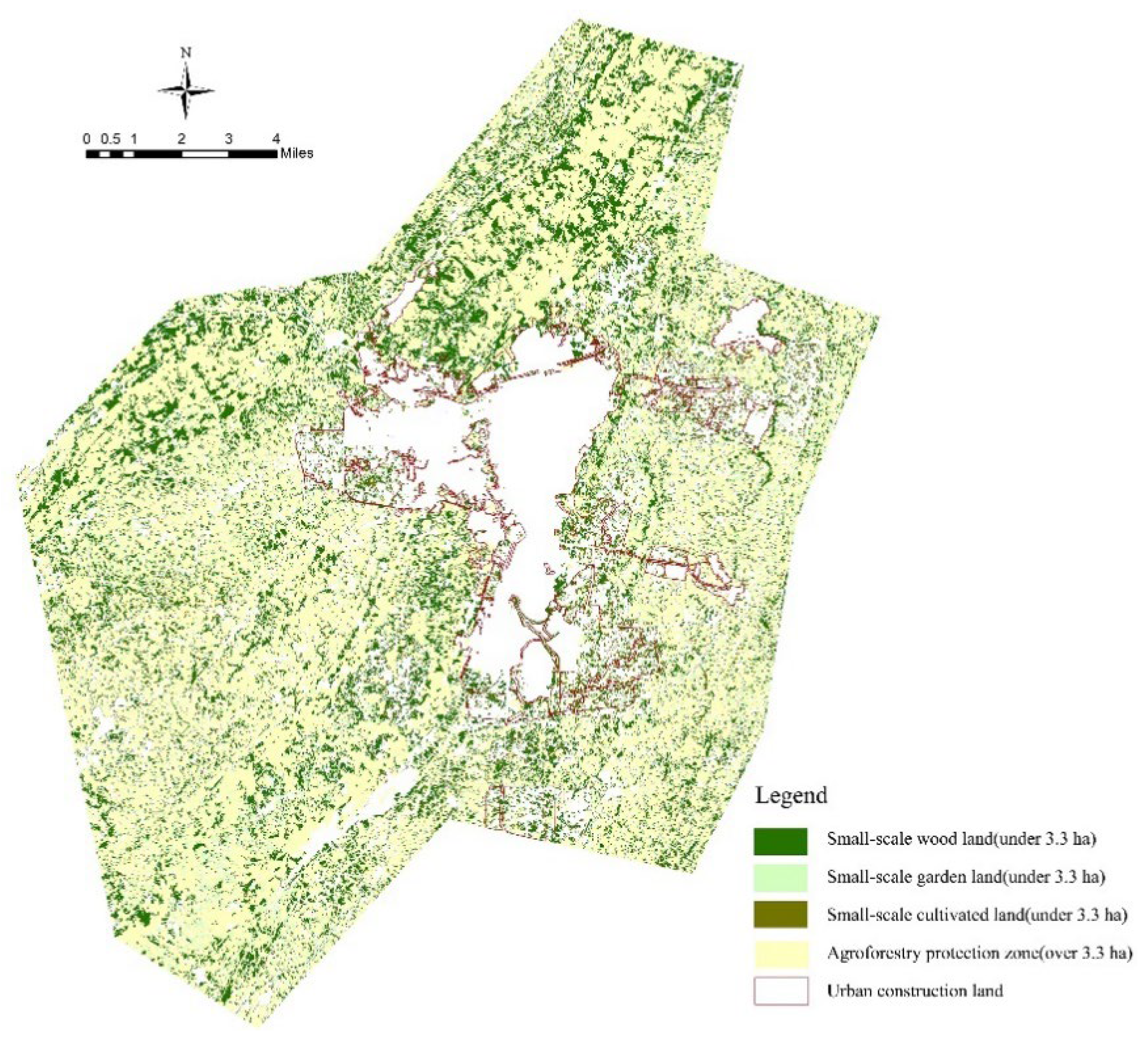
In the first chapter, the object of study has been clearly defined and determined in accordance with laws and regulations and the requirements for the protection of Agricultural and forestry land, it refers to small-scale agroforestry land with an area of less than 3.3 hectares. Therefore, this part of the land use should be statistically screened (
Figure 2).
Through GIS, the space of agriculture and forestry under 3.3 ha is 8694.27 ha, accounting for 75.60% of the total area, and the space of agriculture and forestry over 3.3 ha is 2805.77 ha, accounting for 24.40% of these, 5157.88 hectares (73.4%), 1268.29 hectares (91.1%) and 2268.13 hectares (73.5%) are under 3.3 hectares of arable land, garden land and Woodland respectively (
Table 1). And through the analysis of land use characteristics, SAP spatial gradient of the transformation of the status analysis.
2.4. Sample Selection
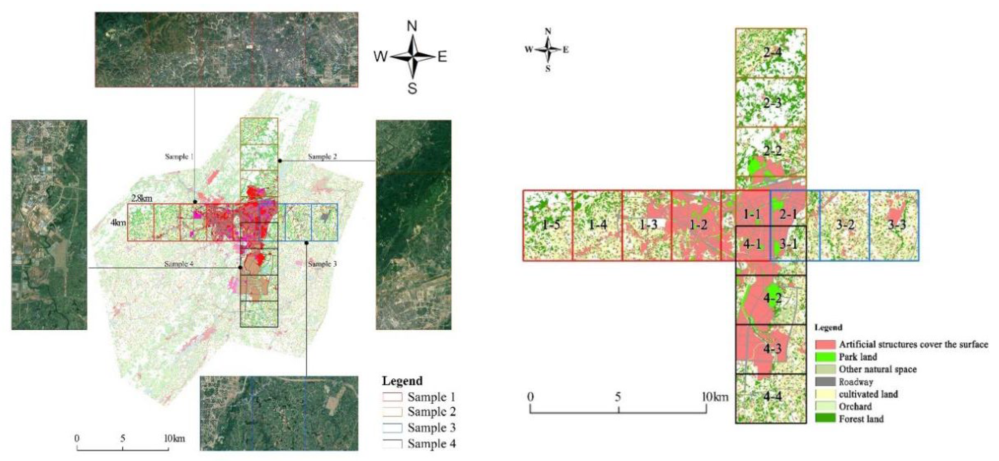
To accurately depict the landscape pattern characteristics of SAP across diverse gradients, a spatially informed approach was adopted. Commencing from the city center area, defined as the starting point of the city’s administrative office space, the investigation extended in four directions within the planning area. Samples were selected with dimensions of 22.4 km × 4 km along both horizontal and vertical axes. These samples were evenly divided into eight squares, each measuring 2.8 km × 4 km (
Figure 3).
2.5. Data Analysis
2.5.1. Calculation of SAP and Agroforestry Elements Landscape Index
Sap is classified according to Chinese land use standards, agricultural and forestry land can be divided into arable land (dryland, paddy field, irrigated land) , garden land(orchard, tea garden land, Oak Garden land, other garden land) , Woodland (arbor Woodland, bamboo Woodland, shrub Woodland, other Woodland) (
Table 2), the change of SAP Landscape Index and the change of various factors were calculated to reflect their transformation characteristics.
Landscape Index can not only simplify the landscape information, but also reflect the structure and spatial configuration of landscape information. It is a simple and applicable quantitative index. In this study, FRAGSTATS4.3 software was used to analyze the spatial landscape pattern of agriculture and forestry in the study area. In this study, the neighborhood search radius was set to 500 m, and the most landscape types were set to 3 types. Based on this, the study divided the agroforestry space into 3M × 3m grids, and calculated the landscape pattern index of Cultivated land, garden land and Woodland within each 2.8 km × 4km plot, three levels of analysis were included: patch, class and landscape. For the need of calculation, the parameters of landscape type, depth effect distance of landscape edge, difference weight of adjacent landscape type and similarity of adjacent landscape type were set. Within this context, the term “landscape type” encompasses arable land, garden land, and woodland. The “landscape edge depth effect distance” denotes the extent of influence exerted by the edge effect of one patch on adjacent patches. The “difference weight of adjacent landscape type” signifies the extent of dissimilarity between two neighboring patches, while the “similarity of adjacent landscape type” quantifies the degree of resemblance between two adjacent patches..
Utilizing the tripartite data, Fragstats 4.3 was employed to compute landscape index characteristics for agroforestry spaces, yielding the Small Agricultural and Forestry Patches (SAP) landscape pattern indices for each segment. The indices encompass patch area (PA), patch density (PD), edge density (ED), largest patch index (LPI), fractal dimension, and aggregation index (AI). These metrics collectively capture the scale, fragmentation, segmentation (spatial distribution), predominant types of agroforestry elements, shape complexity, and connectivity of agroforestry patches (
Table 3).
2.5.2. Statistical Analysis of Natural and Artificial Factors
1). Analysis of topographic and geomorphological factors
The natural succession and disturbance have relatively little influence on the change of the whole agroforestry patch, and the key factor in the mountainous environment is its complex topography, elevation, slope and undulation determine the spatial pattern of agroforestry. Therefore, this paper chooses topography as a natural factor for analysis.
Based on the DEM data of 12.5 m, the elevation, slope and undulation (
Figure 4) were analyzed and calculated by Arcgis 10.2. The slope calculation was obtained by 3D Analyst, relief was calculated by Spatial Analyst Tool-neighborhood analysis-focus statistics. Then, the average values of elevation, slope and fluctuation of each subarea were calculated by Spatial Analyst Tool-regional analysis-regional statistics (
Table 4).
2). Artificial factor analysis
Artificial factors include impervious area, population density, road density, building coverage and so on. The population density can be characterized by the scale of the building’s surface coverage, and the impervious area is actually the superposition of the building’s surface coverage and the road area. In addition, other factors affecting SAP distribution are the construction of existing parks and the excavation of artificial ponds and lakes. First of all, the construction of the park will be combined with the existing distribution of agricultural and forestry resources, choose to occupy these resources to build the park, so it will affect the transformation of SAP status quo, at the same time, artificial pit pond lakes are usually used to irrigate Cultivated land, garden land and part of forestland, and their spatial distribution and scale are likely to affect the spatial pattern of SAP. Therefore, the selection of artificial factors include: building surface coverage, roads, parks, artificial excavation of the pit pond lake.
Based on the data of the third survey, the area scale of road, park, building surface and Artificial pond and lake surface on the urban-rural gradient is calculated (
Table 5).
2.5.3. Correlation Analysis
Due to the small sample size, Spearman correlation analysis was used in this study. Spearman correlation analysis is a nonparametric test proposed by the psychologist Spearman by calculating the Spearman rank correlation coefficient Rs (XI, Yi) and judging the strength of the relationship between two random variables based on the magnitude of the coefficient (Spearman, 2010). Compared with traditional Pearson correlation analysis method, Spearman correlation analysis method is more universal and has been widely used in the study of trade-offs and synergies of ecosystem services (Zhu et al., 2018). Based on the non-linear and non-normal characteristics of geospatial data, the correlation and driving factors of patch landscape index were tested. The mathematical principle is: Let {(XI, Yi)} denote n pairs of data pairs with independent and identical distribution whose parent body is a binary continuous distribution. To arrange XI from small to large, a new set of data pair X (1) < x (2) < x (3) ... < x (N). Where the Yi corresponding to the order statistic of X is called an adjoint of XI. The formula is as follows:
In the formula: Pi Means XI is the K position in the sequence {(XI)} ; K is the rank of XI; similarly, Qi is the rank of Yi. The positive (negative) correlation coefficient indicated that there was an influence relationship among the factors. Rs < 0.7 was a low correlation, 0.7-0.9 was a moderate correlation, and > 0.9 was a high correlation. If P > 0.05, the two functions were independent. The effect of each factor on patch transformation was estimated by Spearman coefficient.
3. Results and Discussion
3.1. The Transformation Characteristics of Agricultural and Forestry Landscape Pattern Gradients
3.1.1. Overall Transformation Characteristics of Agroforestry Patches
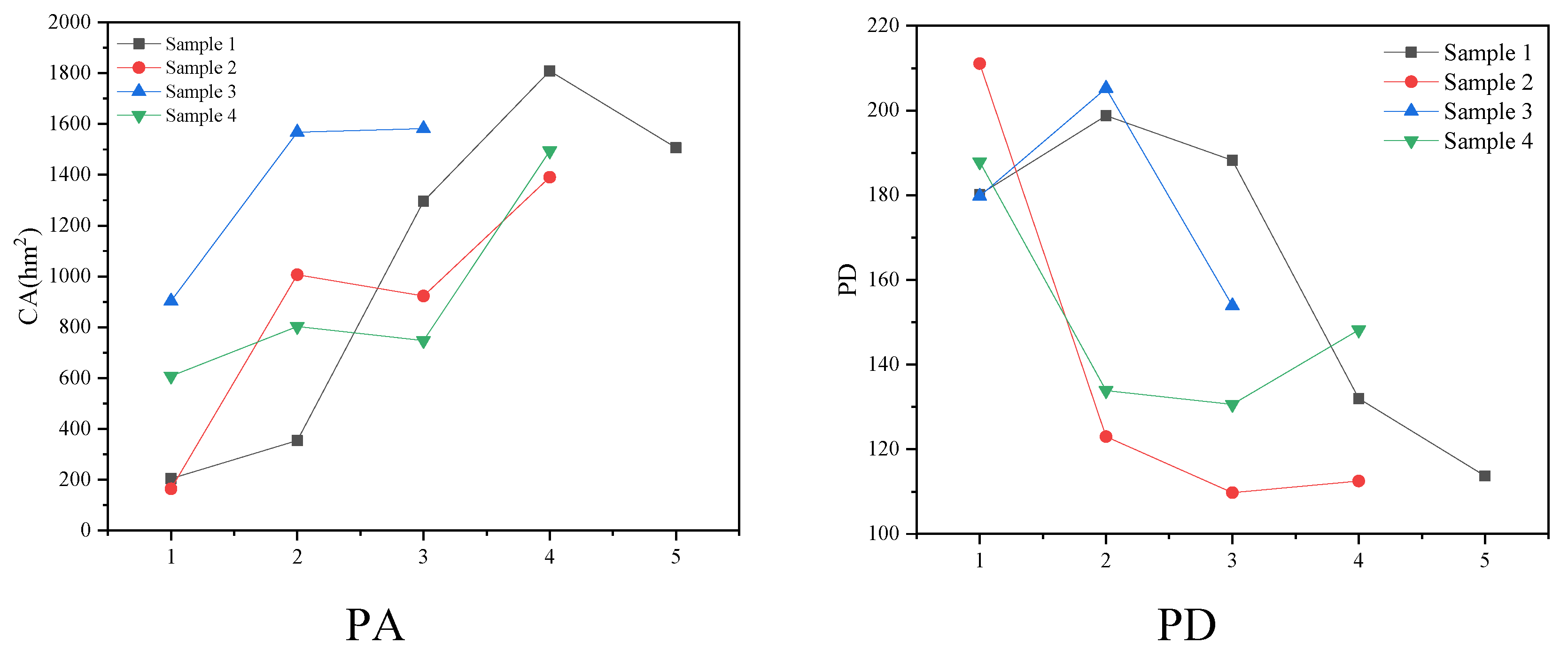
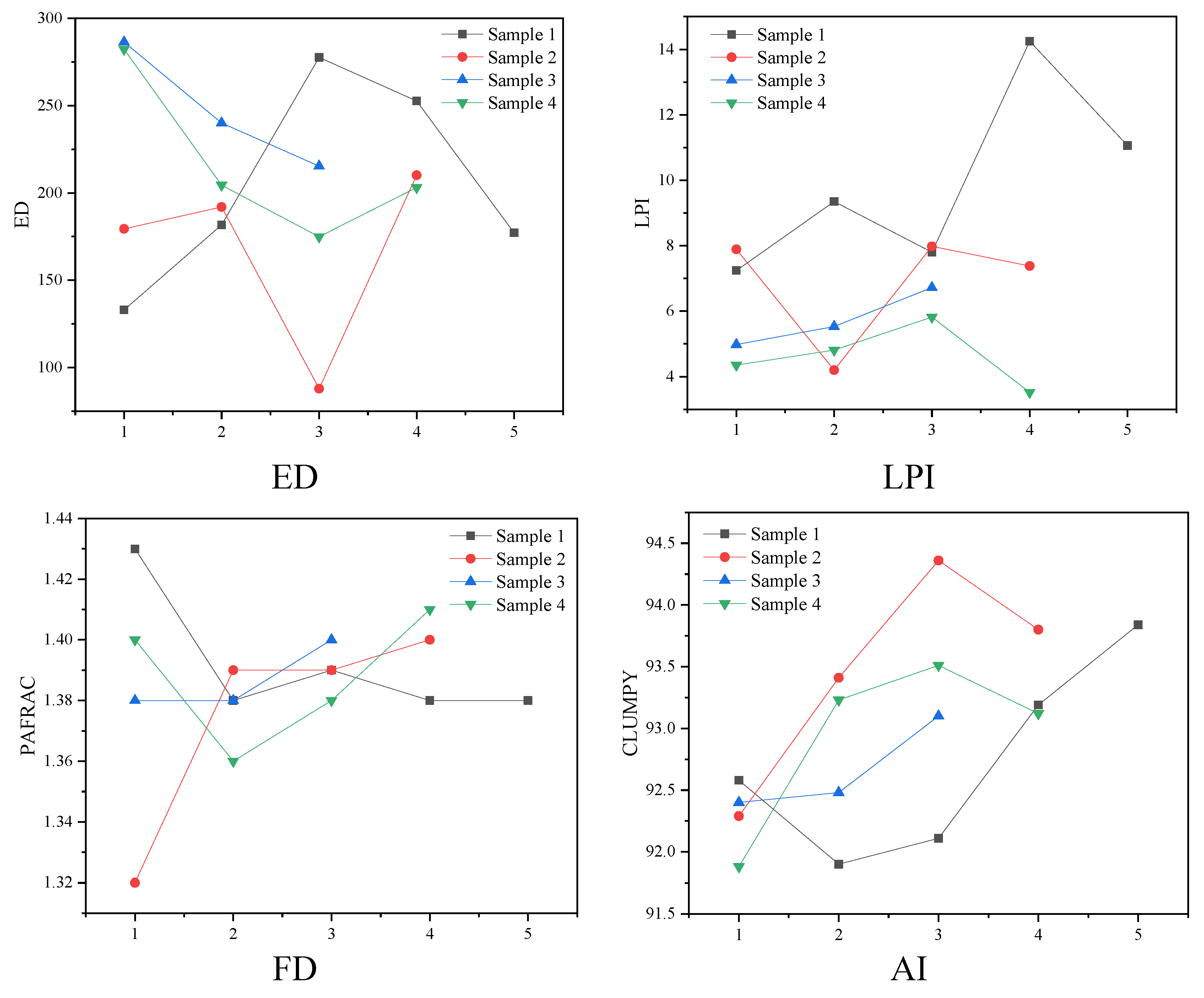
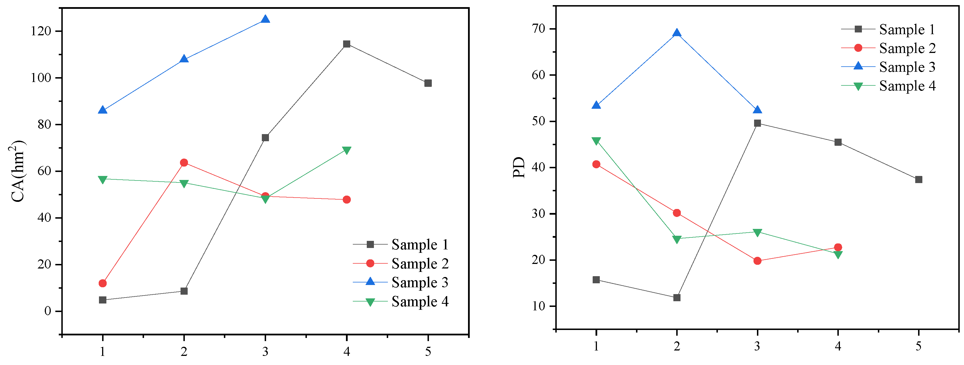
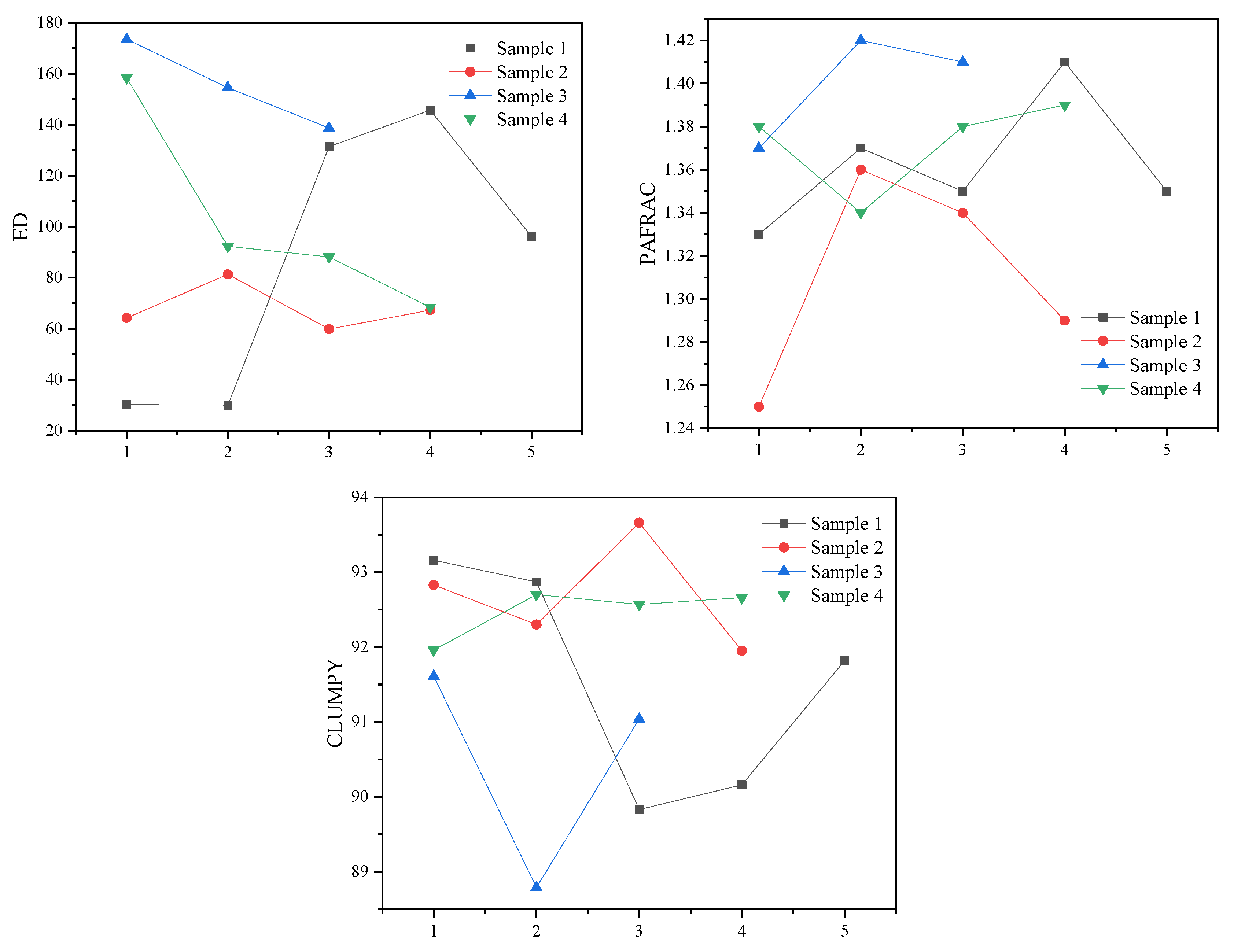
Through the calculation of four samples of landscape index, it is found that there are great differences in different directions of the changes in the agro-forestry landscape index, the overall non-linear changes. The dominant species of landscape in sample 2 were Cultivated land except Woodland. In terms of patch area, density and aggregation index, the four samples showed a similar rule, that is, patch area and aggregation index increased with the increase of the distance from the city, while patch density was opposite, the clustering index was highly negatively correlated with patch density, indicating that the greater the patch area and the lower the fragmentation, the higher the connectivity, which may be due to the increasing distance from the city, the patch of agriculture and forest is less disturbed by human, the intensity of segmentation is less, and the integrity of landscape is higher.
As far as the boundary density is concerned, samples 1 and 2 exhibit curvilinear changes with the increase of urban distance, and the sudden increase of the boundary density of sample 1 in 1-3 may be related to the land-use nature of this section, rural Settlement of Russia is the main area in this area, and arable land is the dominant landscape, which may be due to the complex topography and landform and the local arable land management system. The edge density of sample 2 was also mutated in 2-3. According to the field investigation, 2-3 was distributed in large contiguous and high-lying mountain forests, the distribution was more concentrated. The ED of samples 3 and 4 decreased as the distance between cities increased, that is, the dispersion became smaller and smaller. The ED has a low negative correlation with the aggregation index, that is, the higher the dispersion, the lower the connectivity (
Table 6). This also reflected the higher patch integrity with increasing distance. As for LPI, the landscape dominance of samples 1,3 and 4 were Cultivated land. With the increase of distance from cities, LPI first increased and then decreased, which may be because the proportion of Cultivated land was higher in the rural areas, the closer to the mountains, the greater the proportion of Woodland, leading to a decrease in LPI. The LPI coefficient of sample 2 was the lowest in 2-2, and then increased because of the large proportion of arable land and construction land in this region. The fractal dimension is basically the same in the whole transformation process of small-scale agroforestry patch, but the fractal dimension is smaller in the 2-1 section of Sample 2, the possible reason is that a large area of agricultural and forest patch is kept as an open space in the urban area, which is not occupied by force, thus it can be effectively protected (
Figure 5).
From the above results, we can see that with the increase of the distance between SAP and cities, the landscape index shows the characteristics of different transformation, however, the specific reasons for this are explained in more detail.
3.1.2. Transformation Characteristics of Agricultural and Forestry Elements
1). Transformation characteristics of landscape index of wood land
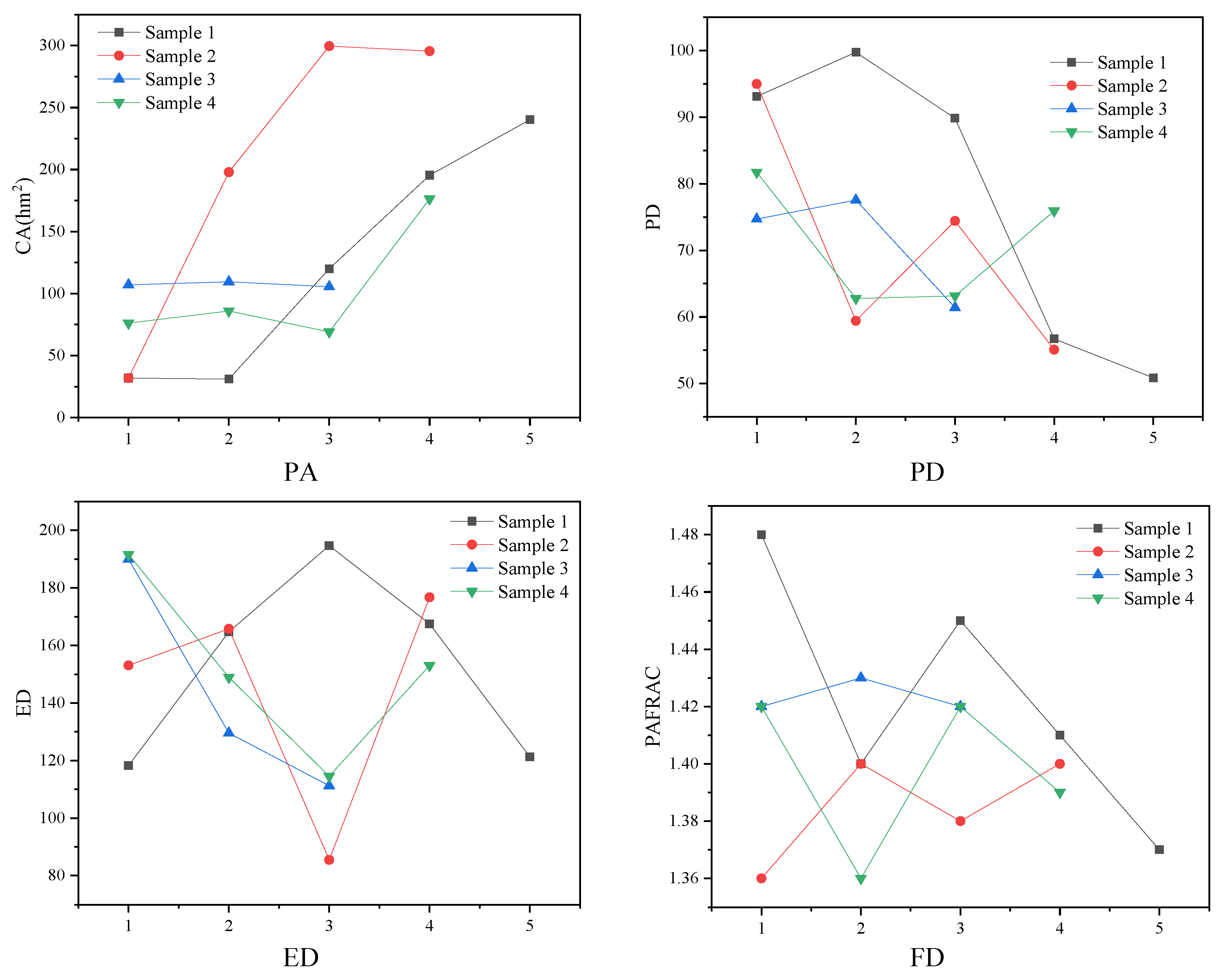
The Woodland patch area, density, and aggregation index exhibited a convoluted transformation along the gradient. Specifically, patch area (PA) and patch density (PD) displayed a negative correlation, while the aggregation index showed a positive correlation. This implies that, as the distance from the city increases, the patch area enlarges, fragmentation diminishes, and connectivity intensifies. Additionally, there exists a negative correlation between the aggregation index and fractal dimension, signifying that higher connectivity corresponds to lower shape complexity (
Table 7). Other landscape indices displayed irregular transformation characteristics. Firstly, the edge density (ED) analysis revealed that the transformation characteristics of sample 1 initially increased, then decreased, reaching a peak between 1-1 and 1-3, and subsequently decreased to a trough. This pattern suggests that urban fringe areas and affected rural zones, characterized by intense human activity, experience irregular woodland erosion, resulting in heightened fragmentation. A similar trend was observed for Sample 2, where dense mountain forest distribution in segment 2-3 initially decreased sharply, then increased. Conversely, Samples 3 and 4 exhibited a relatively regular decreasing transformation, with dispersion decreasing as the distance from the city increased. Secondly, the fractal dimension of Samples 1 and 4 decreased, indicating simpler shapes and less artificial interference. In contrast, the fractal dimension of Sample 2 increased, suggesting more complex shapes and greater artificial interference. Notably, in urban areas, the fractal dimension of woodland patches was the smallest, possibly because urban woodlands are considered natural and recreational parks, subject to less intensive development. Conversely, in rural areas, the likelihood of erosion and disturbance increases (
Figure 6).
The transformation rule of forest patch is similar to SAP. With the increase of the distance from the city, the bigger the patch area, the smaller the fragmentation and dispersion, the higher the connectivity, the lower the shape complexity, and the higher the LPI. From the characteristics of Woodland transformation, it can be seen that the intensity of Woodland disturbance changes with the increase of the distance from the city, for example, the conversion of Woodland from flat land to construction land or arable land, leaving behind a complex terrain, difficult to develop the remaining Woodland, therefore, in order to avoid further erosion of Woodland outside the city, to avoid further erosion.
2). Transformation characteristics of patch landscape index of Cultivated land
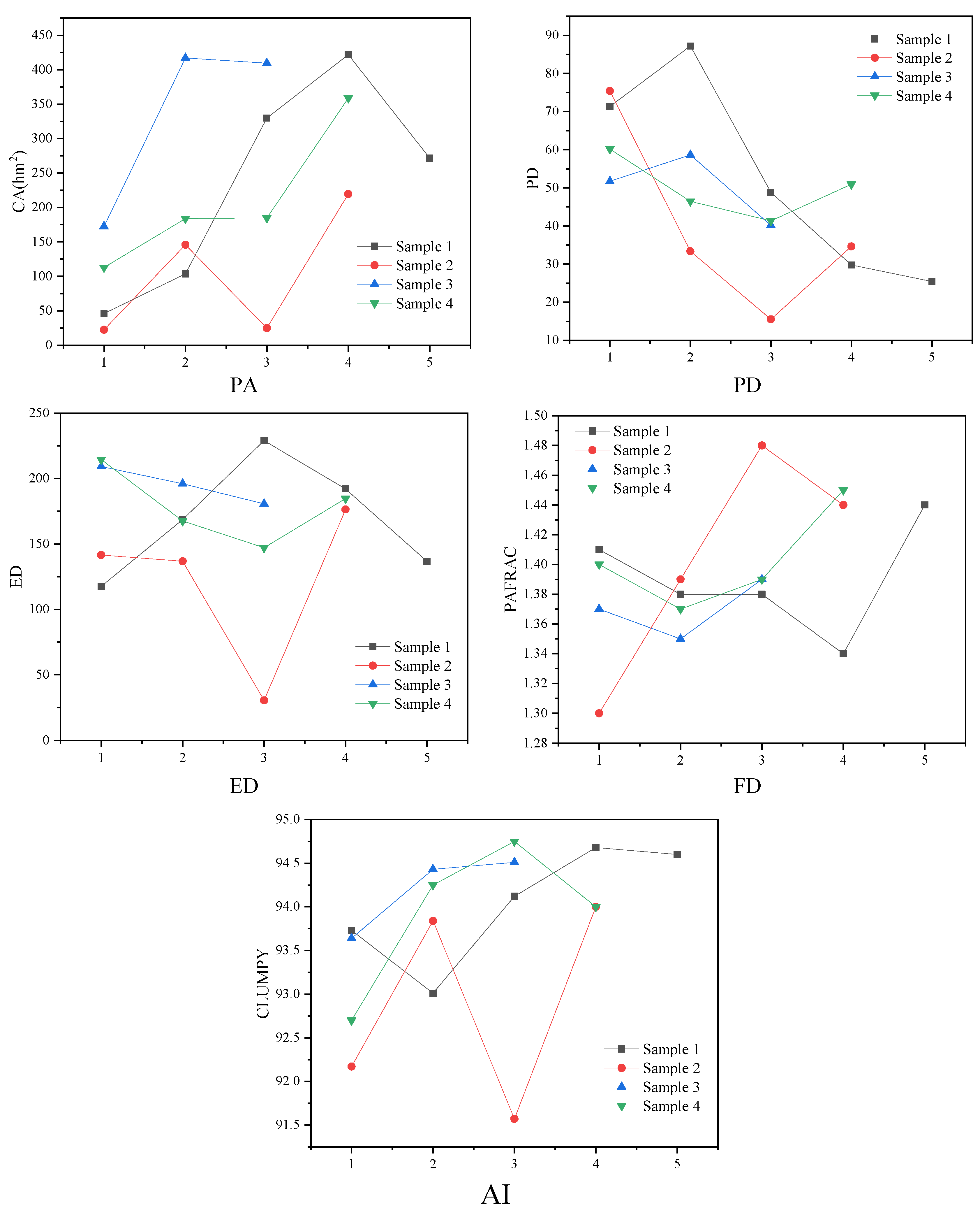
The patch area, density and aggregation index of Cultivated land showed a zigzag pattern, and the patch area as a whole changed irregularly with the increase of the distance from the city, it conforms to the normal law of change, because of the surrounding countryside cultivated land, across the city is rural land, and then to the primary natural forest-based. Sample 2 rises first, then falls and rises again, which may be related to topography and topography. As analyzed above, 2-3 is a large area of mountain forest, which is difficult to be cultivated. Therefore, the Cultivated land is smaller, and the cross-mountain forest enters the rural section, the scale of cropland increased. Sample 4 is rising slowly and then increasing rapidly, which may be related to the direction of urban development. If the distance of sample selection is further expanded, the Cultivated land will decrease while the distance between the Cultivated land and the city is further increased (
Figure 7).
Moreover, the patch area exhibited a positive correlation with the aggregation index and a negative correlation with Edge Density (ED). Specifically, larger patch areas were associated with higher connectivity and lower dispersion (
Table 8). This reveals distinctions in the transformation characteristics between Cultivated Land patches and Woodland patches. In the case of Cultivated Land patches, the patch area may not undergo significant changes, but the increase in the total scale could be attributed to topography impeding the concentration of cultivated land. Consequently, larger scales were linked to higher dispersion. Connectivity, on the other hand, increased through connections via field roads and water system corridors. In the landscape index of Cultivated Land patches, the fractal dimension exhibited a rising trend, indicating that as one moves farther from the city, the shape becomes more complex. This trend may be attributed to inherent characteristics of Cultivated Land, resulting in increasingly intricate shapes.
According to the gradient transformation characteristics of Cultivated land patch, Cultivated land shows the trend of increasing first and then decreasing, except for the irregular changes caused by topography and geomorphology. The characteristics of patch transformation in SAP are more obvious because of human factors. The concentrated patches have been designated as protected areas, and the remaining patches in SAP are scattered patches with an area of less than 3.3 hectare, with the expansion of the city, it is extremely easy to be occupied by construction land, therefore, the protection of this part of cultivated land patch should also develop appropriate policies and measures, otherwise, otherwise, small patches of arable land will only disappear.
3). Landscape index transformation characteristics of garden land
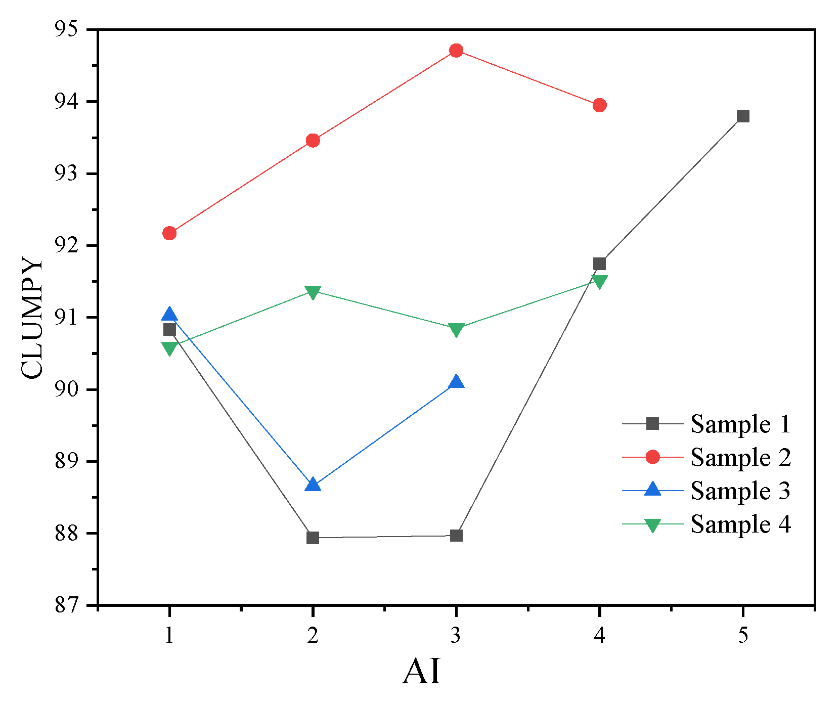
Garden land and cultivated land patches similar to artificial cultivation of orchards, tea plantations and other agricultural land. The patch landscape index of garden land plot shows a relatively regular transformation rule, and there is a great correlation among the indices. The patch area increased with the increase of the distance from the city, and the patch area first increased and then decreased in sample 2, which was also related to the distribution of large mountain forests in sample 2-3. The patch area had a moderate positive correlation with patch density and ED, a low positive correlation with fractal dimension and a moderate negative correlation with aggregation index, the higher the fragmentation, dispersion and shape complexity, the lower the connectivity (
Table 9). It shows that the plantation of garden land is not concentrated and continuous, but selective embedded planting, with the increase of the scale, the degree of fragmentation and dispersion is higher, which is consistent with the phenomenon of field investigation, which is usually embedded in Cultivated land and Woodland, this leads to lower connectivity (
Figure 8).
The transformation characteristics of patch landscape index were different from those of Woodland and cropland. With the increase of patch size, not only the fragmentation and dispersion of patch increase, but also the connectivity and shape complexity become lower. The reason for this transformation is closely related to the planting attributes of garden land patches. Close to cities, garden land patches are small in scale, but low in fragmentation and dispersion, and high in connectivity, because they are planted in relatively small quantities, however, the increase of scale is only in the total amount, not in the single area, and it is difficult to form high aggregation and connectivity.
3.2. Drivers of Gradient Transformation of Agroforestry Landscape Patterns
3.2.1. The Driving Factors of the Overall Transformation of Agroforestry Landscape Pattern
The results showed that the driving degree of landform to agroforestry landscape index was weak, and the relationship between patch density and average undulation was P < 0.05, RS was -0.544, which had statistical significance, it can be concluded that there is a low degree of negative correlation between plaque density and mean fluctuation, that is, the greater the fluctuation, the lower the plaque density and the lower the fragmentation. In addition, elevation, slope and undulation have a low degree of correlation, indicating that topography and geomorphology affect the distribution pattern of regional agroforestry elements. The area, density and aggregation index of agricultural and forestry patches were significantly affected by human activities. The patch area showed a significant moderate negative correlation with road size, park area and building surface, the patch density has a low degree of positive correlation with the building surface and the road scale, while the aggregation index has a low degree of negative correlation with the building surface and the road scale, this indicates that the patch landscape index is more affected by human factors. There was no significant correlation between edge density, LPI and fractal dimension and human factors (
Table 10).
3.2.2. Drivers of Transformation of Each Element Landscape Pattern.
1). Analysis of driving factors of Woodland conversion
The results showed that the patch index of Woodland was affected by topography and human factors. The patch area and density were slightly affected by Artificial factors, and the aggregation index was positively correlated with elevation, slope and undulation, and negatively correlated with the building surface and the scale of Kengtang Lake. It shows that the area conversion of Woodland is closely related to elevation, and the larger the area, the higher the elevation, the higher the slope and undulation, and the less the road, Park and building surface. In addition, the greater the degree of fragmentation and connectivity, the lower the elevation, slope, and undulation, and the larger the scale of roads and buildings. It shows that the higher the elevation, slope and fluctuation, the more difficult the land use, but the better the terrain environment is often divided artificially (
Table 11).
2). Driver factor analysis of Cultivated land conversion
The Cultivated land was significantly affected by Artificial factors, especially the area and density of Cultivated land, which had a low negative correlation with road scale, park land and building surface, and a moderate positive correlation with artificial ponds and lakes, this is also related to the characteristics of the layout of Cultivated land in the mountains, usually in the cultivated land around the excavation of ponds for irrigation. The patch accumulation index of Cultivated land was positively correlated with the surface of artificial ponds and lakes (
Table 12).
3). Analysis of driving factors of garden land conversion
The patch area and fractal dimension were significantly affected by human factors. The patch area has a low negative correlation with the size of roads and parks, a low positive correlation with the surface of artificial ponds and lakes, and a moderate positive correlation with the fractal dimension. Garden land is similar to Cultivated land, including orchards, tea garden lands and other kinds of cultivated agricultural land, artificial pit pond lake surface excavation for irrigation, its spatial layout affects the shape of the garden land complex degree, the greater the number of ponds, the greater the probability of plantation (
Table 13).
3.3. Study Limitations
There are three limitations in this paper: first, although the characteristics of landscape pattern transformation of SAP and its elements have been described, however, there are still some problems in the study, such as the small number of samples and the small gradient distance between urban and rural areas, the results are more accurate. Secondly, the selection of influencing factors of SAP can be more diversified, and the changes of agroforestry landscape pattern may be influenced by other factors, examples include urban development policies and future directions (Moreau, 2021) , Typhoons and earthquakes (Lin et al. , 2006) , Artificial and natural fires (Kashian et al. , 2004) , therefore, all kinds of relevant factors should be considered in order to make SAP protection decision more reasonable. Finally, this paper only explores the transformation characteristics of SPA landscape pattern from space, in fact, it is also affected by the time change, the landscape index of the same plot will be different at different time (Southworth et al., 2002) , in order to understand the characteristics of SAP transformation, we must study it from the two dimensions of time and space, which is the content to be further improved in the future.
4. Conclusions
This study investigates the characteristics and influencing factors of SAP transformation in mountain cities along the urban-rural gradient. The findings indicate a non-linear transformation in the landscape pattern of small-scale agricultural and forestry patches in mountainous areas. The total patch area increases from urban to rural areas, accompanied by lower fragmentation and dispersion, higher connectivity, and relatively small changes in fractal dimension. Furthermore, landscape dominance exhibits an increase. These transformation characteristics highlight substantial variations in SAP landscape patterns across distinct urban-rural gradients. Proximity to urban construction areas correlates with smaller scales, higher degrees of fragmentation and dispersion, and lower connectivity. Consequently, conservation efforts and strategies need to account for these significant differences. For SAP near urban areas, the focus should be on artificial ecological restoration, utilizing landscape corridors to connect fragmented agricultural and forest patches and create a green infrastructure network. In contrast, for SAP distant from cities, emphasis should be on strengthening protection measures, delineating protection boundaries, and formulating specific control rules.
In the transformation characteristics of agroforestry elements, the patch area, density and aggregation index of Woodland showed a tortuous regularity along the gradient, that is, the bigger the distance from the city, the bigger the patch area, the smaller the fragmentation and the higher the connectivity, the shape complexity was lower. The patch area, density and aggregation index of Cultivated land showed a zigzag pattern of regular transformation. The patch area showed a moderate positive correlation with the aggregation index, and a low positive correlation with ED, the higher the connectivity, the higher the dispersion. The patch landscape index of garden land plot showed a relatively regular transformation rule, and there was a great correlation among the indices. The patch area was similar to that of Cultivated land and Woodland, that is, it increased, and had positive correlation with patch density, Ed and fractal dimension, and had moderate negative correlation with aggregation index, the higher the fragmentation, dispersion and shape complexity, the lower the connectivity.
There is a low negative correlation between PD and mean fluctuation, that is, the greater the fluctuation, the lower the fragmentation. However, the area and density of SAP were significantly affected by the scale of roads, parks and buildings. In the factors of agriculture and forestry, forestland is affected by landform and Artificial factors to the same degree, while the patch area, fragmentation and connectivity of forestland are affected significantly by elevation, slope and undulation, the higher the elevation, slope and fluctuation, the more difficult the land use, but the flat terrain is often divided by people. However, the Cultivated land and garden land are influenced by human factors, especially by topography and landform. The spatial distribution and scale of artificial pond lake are in direct proportion to the scale of Cultivated land and garden land. Therefore, the methods of conservation and spatial planning are different according to different agroforestry factors.
Author Contributions
Conceptualization, Z.X; methodology, C.C; software, Z.X.; validation, L.Y., J.Y. and C.C; formal analysis, C.C; investigation, C.C; resources, Z.X; data curation, C.C; writing-original draft preparation, C.C; writing-review and editing, L.Y; visualization, Z.X; supervision, J.Y; project administration, Z.X; funding acquisition, Z.X. All authors have read and agreed to the published version of the manuscript.
Data Availability Statement
The data presented in this study are available on request from the corresponding author.
Acknowledgments
We appreciate the assistance of the Natural Resources Bureau of Yongchuan District, Chongqing for providing the base data..
Conflicts of Interest
The authors declare no conflict of interest.
References
- Abdullah, A.; Khan, S.M.; Pieroni, A.; Haq, A.; Haq, Z.U.; Ahmad, Z.; Sakhi, S.; Hashem, A.; Al-Arjani, A.-B.F.; Alqarawi, A.A.; et al. A Comprehensive Appraisal of the Wild Food Plants and Food System of Tribal Cultures in the Hindu Kush Mountain Range; a Way Forward for Balancing Human Nutrition and Food Security. Sustainability 2021, 13, 5258. [Google Scholar] [CrossRef]
- Bhatta, B. , 2010. Causes and Consequences of Urban Growth and Sprawl, in: Bhatta, B. (Ed.), Analysis of Urban Growth and Sprawl from Remote Sensing Data, Advances in Geographic Information Science. Springer, Berlin, Heidelberg, pp. 17–36. [CrossRef]
- Burton, M.L.; Samuelson, L.J.; Pan, S. Riparian woody plant diversity and forest structure along an urban-rural gradient. Urban Ecosyst. 2005, 8, 93–106. [Google Scholar] [CrossRef]
- Cardille, J.A. , Turner, M.G., 2017. Understanding Landscape Metrics, in: Gergel, S.E., Turner, M.G. (Eds.), Learning Landscape Ecology: A Practical Guide to Concepts and Techniques. Springer, New York, NY, pp. 45–63. [CrossRef]
- Carreiro, M.M.; Tripler, C.E. Forest Remnants Along Urban-Rural Gradients: Examining Their Potential for Global Change Research. Ecosystems 2005, 8, 568–582. [Google Scholar] [CrossRef]
- Cifaldi, R.L.; Allan, J.D.; Duh, J.; Brown, D.G. Spatial patterns in land cover of exurbanizing watersheds in southeastern Michigan. Landsc. Urban Plan. 2004, 66, 107–123. [Google Scholar] [CrossRef]
- Clergeau, P.; Savard, J.-P.L.; Mennechez, G.; Falardeau, G. Bird Abundance and Diversity along an Urban-Rural Gradient: A Comparative Study between Two Cities on Different Continents. Condor 1998, 100, 413–425. [Google Scholar] [CrossRef]
- Farina, A. The Cultural Landscape as a Model for the Integration of Ecology and Economics. BioScience 2000, 50, 313–320. [Google Scholar] [CrossRef]
- Forman, R.T.T. Land Mosaics: The Ecology of Landscapes and Regions, 1st ed.; Cambridge University Press: Cambridge, UK, 1995; ISBN 978-0-521-47980-6. [Google Scholar]
- Garaffa, P.I.; Filloy, J.; Bellocq, M.I. Bird community responses along urban–rural gradients: Does the size of the urbanized area matter? Landsc. Urban Plan. 2009, 90, 33–41. [Google Scholar] [CrossRef]
- Halada, L.; Evans, D.; Romão, C.; Petersen, J.-E. Which habitats of European importance depend on agricultural practices? Biodivers. Conserv. 2011, 20, 2365–2378. [Google Scholar] [CrossRef]
- Kaminski, A.; Bauer, D.M.; Bell, K.P.; Loftin, C.S.; Nelson, E.J. Using landscape metrics to characterize towns along an urban-rural gradient. Landsc. Ecol. 2021, 36, 2937–2956. [Google Scholar] [CrossRef]
- Kashian, D.M.; Tinker, D.B.; Turner, M.G.; Scarpace, F.L. Spatial heterogeneity of lodgepole pine sapling densities following the 1988 fires in Yellowstone National Park, Wyoming, USA. Can. J. For. Res. 2004, 34, 2263–2276. [Google Scholar] [CrossRef]
- Körner, C. Mountain Biodiversity, Its Causes and Function. AMBIO 2004, 33, 11–17. [Google Scholar] [CrossRef]
- Li, H.; Reynolds, J.F. A Simulation Experiment to Quantify Spatial Heterogeneity in Categorical Maps. Ecology 1994, 75, 2446–2455. [Google Scholar] [CrossRef]
- Li, Y.; Li, Y.; Westlund, H.; Liu, Y. Urban–rural transformation in relation to cultivated land conversion in China: Implications for optimizing land use and balanced regional development. Land Use Policy 2015, 47, 218–224. [Google Scholar] [CrossRef]
- Lin, Y.-P.; Chang, T.-K.; Wu, C.-F.; Chiang, T.-C.; Lin, S.-H. Assessing Impacts of Typhoons and the Chi-Chi Earthquake on Chenyulan Watershed Landscape Pattern in Central Taiwan Using Landscape Metrics. Environ. Manag. 2006, 38, 108–125. [Google Scholar] [CrossRef] [PubMed]
- López, T.d.M.; Aide, T.M.; Thomlinson, J.R. Urban Expansion and the Loss of Prime Agricultural Lands in Puerto Rico. AMBIO 2001, 30, 49–54. [Google Scholar] [CrossRef]
- Mao, D.; Wang, Z.; Wu, J.; Wu, B.; Zeng, Y.; Song, K.; Yi, K.; Luo, L. China's wetlands loss to urban expansion. Land Degrad. Dev. 2018, 29, 2644–2657. [Google Scholar] [CrossRef]
- McDonnell, M. , Pickett, S.T.A., Groffman, P., Bohlen, P., Pouyat, R., Zipperer, W., Parmelee, R., Carreiro, M., Medley, K., 2008. Ecosystem Processes Along an Urban-to-Rural Gradient, in: Urban Ecosystems. pp. 299–313. [CrossRef]
- Moreau, M. Transect urbanism: readings in human ecology. Urban Res. Pr. 2021, 14, 483–484. [Google Scholar] [CrossRef]
- Niemelä, J.; Kotze, D.J.; Venn, S.; Penev, L.; Stoyanov, I.; Spence, J.; Hartley, D.; de Oca, E.M. Carabid beetle assemblages (Coleoptera, Carabidae) across urban-rural gradients: an international comparison. Landsc. Ecol. 2002, 17, 387–401. [Google Scholar] [CrossRef]
- Plieninger, T. , Bieling, C., 2013. Resilience-Based Perspectives to Guiding High-Nature-Value Cultivated land through Socioeconomic Change. Ecology and Society 18.
- Qian, S.; Qin, D.; Wu, X.; Hu, S.; Hu, L.; Lin, D.; Zhao, L.; Shang, K.; Song, K.; Yang, Y. Urban growth and topographical factors shape patterns of spontaneous plant community diversity in a mountainous city in southwest China. Urban For. Urban Green. 2020, 55, 126814. [Google Scholar] [CrossRef]
- Sanesi, G.; Colangelo, G.; Lafortezza, R.; Calvo, E.; Davies, C. Urban green infrastructure and urban forests: a case study of the Metropolitan Area of Milan. Landsc. Res. 2017, 42, 164–175. [Google Scholar] [CrossRef]
- Southworth, J.; Nagendra, H.; Tucker, C. Fragmentation of a Landscape: Incorporating landscape metrics into satellite analyses of land-cover change. Landsc. Res. 2002, 27, 253–269. [Google Scholar] [CrossRef]
- Spearman, C. The proof and measurement of association between two things. Leuk. Res. 2010, 39, 1137–1150. [Google Scholar] [CrossRef] [PubMed]
- Su, S.; Hu, Y.; Luo, F.; Mai, G.; Wang, Y. Farmland fragmentation due to anthropogenic activity in rapidly developing region. Agric. Syst. 2014, 131, 87–93. [Google Scholar] [CrossRef]
- Tan, S.; Heerink, N.; Qu, F. Land fragmentation and its driving forces in China. Land Use Policy 2006, 23, 272–285. [Google Scholar] [CrossRef]
- Tlapáková, L.; Stejskalová, D.; Karásek, P.; Podhrázská, J. Landscape Metrics as a Tool for Evaluation Landscape Structure – Case Study Hustopeče. Eur. Countrys. 2013, 5. [Google Scholar] [CrossRef]
- Uuemaa, E.; Antrop, M.; Roosaare, J.; Marja, R.; Mander, U. Landscape Metrics and Indices: An Overview of Their Use in Landscape Research. Living Rev. Landsc. Res. 2009, 3, 1–28. [Google Scholar] [CrossRef]
- van Vliet, J. Direct and indirect loss of natural area from urban expansion. Nat. Sustain. 2019, 2, 755–763. [Google Scholar] [CrossRef]
- Walz, U. Landscape Structure, Landscape Metrics and Biodiversity. Living Rev. Landsc. Res. 2011, 5. [Google Scholar] [CrossRef]
- Wear, D.N. , Turner, M.G., Naiman, R.J., 1998. Land Cover Along an Urban–Rural Gradient: Implications for Water Quality. Ecological Applications 8, 619–630. [CrossRef]
- Xu, J.; Ma, E.T.; Tashi, D.; Fu, Y.; Lu, Z.; Melick, D. Integrating Sacred Knowledge for Conservation: Cultures and Landscapes in Southwest China. Ecol. Soc. 2005, 10. [Google Scholar] [CrossRef]
- Yang, X.; Liu, Z. Quantifying landscape pattern and its change in an estuarine watershed using satellite imagery and landscape metrics. Int. J. Remote. Sens. 2005, 26, 5297–5323. [Google Scholar] [CrossRef]
- Yang, Y.; Guangrong, S.; Chen, Z.; Hao, S.; Zhouyiling, Z.; Shan, Y. Quantitative analysis and prediction of urban heat island intensity on urban-rural gradient: A case study of Shanghai. Sci. Total. Environ. 2022, 829, 154264. [Google Scholar] [CrossRef] [PubMed]
- Zhu, Q.Y. , Hu, W., Zhao Z.S. 2018. Dynamic analysis of multi-function trade-offs and synergistic spatio-temporal patterns of Cultivated land: a case study of Hubei province. Economic geography38,143-153. [CrossRef]
- Huang, G.Y. 2005. Ecological thinking on the spatial structure of mountain cities. Urban Planning 57-63.
Figure 1.
The location of study area. The upper right figure illustrates the geographic location of Chongqing Municipality within China, while the lower right figure indicates the position of Yongchuan District within Chongqing Municipality. The left figure depicts the location of the research area within Yongchuan District, including the extent of urban built-up areas within the research area.
Figure 2.
Identification of small-scale agricultural and forestry land. Using ArcGIS 10.2, small-scale agroforestry land under 3.3 hectares were selected, which are intricately intertwined with agroforestry protection zones, spanning across both urban construction areas and the peripheries of cities.
Figure 3.
Sample partitioning. Spatial transects of urban-rural areas were delineated from the city center to the boundaries of natural conservation areas, partitioned evenly in 2.8 km × 4 km intervals along the cardinal directions of southeast, southwest, northeast, and northwest.
Figure 3.
Sample partitioning. Spatial transects of urban-rural areas were delineated from the city center to the boundaries of natural conservation areas, partitioned evenly in 2.8 km × 4 km intervals along the cardinal directions of southeast, southwest, northeast, and northwest.
Figure 4.
Analysis of topographic and geomorphological. Figure a represents the elevation within the spline space, Figure b denotes the slope within the spline space, and Figure c refers to the undulation within the spline space.
Figure 4.
Analysis of topographic and geomorphological. Figure a represents the elevation within the spline space, Figure b denotes the slope within the spline space, and Figure c refers to the undulation within the spline space.
Figure 5.
Landscape index transformation of SAP. The figure illustrates the trend of spline space landscape index transformation for small-scale agricultural and forestry areas in different directions.
Figure 5.
Landscape index transformation of SAP. The figure illustrates the trend of spline space landscape index transformation for small-scale agricultural and forestry areas in different directions.
Figure 6.
Representation of woodland landscape index transformation. The figure illustrates the trend of spline space landscape index transformation for small-scale woodland in different directions.
Figure 6.
Representation of woodland landscape index transformation. The figure illustrates the trend of spline space landscape index transformation for small-scale woodland in different directions.
Figure 7.
Representation of cultivated land landscape index transformation. The figure illustrates the trend of spline space landscape index transformation for small-scale cultivated land in different directions.
Figure 7.
Representation of cultivated land landscape index transformation. The figure illustrates the trend of spline space landscape index transformation for small-scale cultivated land in different directions.
Figure 8.
Representation of garden land landscape index transformation. The figure illustrates the trend of spline space landscape index transformation for small-scale garden land in different directions.
Figure 8.
Representation of garden land landscape index transformation. The figure illustrates the trend of spline space landscape index transformation for small-scale garden land in different directions.
Table 1.
Yongchuan Agricultural and forestry space statistics of various types of land area.
Table 1.
Yongchuan Agricultural and forestry space statistics of various types of land area.
| Type |
Woodland |
Cultivated land |
Garden land |
| Area (hm2) |
Percentage (%) |
Area (hm2) |
Percentage (%) |
Area (hm2) |
Percentage (%) |
| Over 3.3 ha |
815.8 |
26.45 |
1865.4 |
26.56 |
124.54 |
8.94 |
| Under 3.3 ha |
2268.13 |
73.55 |
5157.88 |
73.44 |
1268.29 |
91.06 |
Table 2.
classification of land uses for Territorial Space Survey, planning and use control.
Table 2.
classification of land uses for Territorial Space Survey, planning and use control.
| Cultivated land |
Paddy fields |
| Irrigated land |
| Drylands |
| Garden land |
Orchards |
| Tea Garden land |
| Oak Park |
| Other garden land plots |
| Woodland |
Arbor Woodland |
| Bamboo Woodland |
| Shrub Woodland |
| Other Woodland |
Table 3.
description of various types of landscape indices.
Table 3.
description of various types of landscape indices.
| Landscape indices |
Formula |
Explain |
Explain |
| Patch area (PA) |
|
The area of IJ for plaque |
CA can reflect the change of agroforestry scale on urban-rural gradient |
| Plaque density (PD) |
|
Ni is the number of patches contained by patch type I, and a is the area of the whole landscape, including the background within the landscape. Units are 1/100 HM2 |
The patch density, defined as the number of patches per unit area, serves as an indicator of the fragmentation level in agricultural and forestry patches. |
| Edge density (ED) |
Ed = E/A |
E is the total perimeter of the plaque, and a is the total area of the plaque |
The higher the boundary density is, the higher the land-use type is divided and the more dispersed the layout is |
| Largest plaque index (LPI) |
|
Aij represents the area of patch ij; and A denotes the total landscape area, encompassing both the landscape interior and background. |
Reflecting dominant land-use patch types and landscape dominance in different partitions |
| Fractal dimension (FD) |
|
For perimeter of plaque ij; for area of plaque ij |
To quantify the complexity of patch shapes, values closer to 1 indicate simpler shapes, while values closer to 2 signify more intricate shapes, indicative of heightened artificial influence. |
| Aggregation index (AI) |
|
GI is the similar adjacency ratio, pi is the area proportion of the patch type in the landscape |
Indicates the level of connectivity between patches; higher values denote increased connectivity. |
Table 4.
Statistics of gradient transformation of surface terrain data.
Table 4.
Statistics of gradient transformation of surface terrain data.
| Samples |
Average elevation |
Average slope |
Average Rise and fall |
| 1-1 |
276.41 |
5.21 |
27.89 |
| 1-2 |
279.58 |
6.17 |
35.56 |
| 1-3 |
283.26 |
5.16 |
25.11 |
| 1-4 |
293.68 |
8.13 |
43.12 |
| 1-5 |
345.34 |
12.32 |
84.50 |
| 2-1 |
281.75 |
5.47 |
28.65 |
| 2-2 |
351.17 |
12.27 |
88.75 |
| 2-3 |
627.08 |
20.11 |
172.52 |
| 2-4 |
412.84 |
15.65 |
127.00 |
| 3-1 |
304.28 |
7.76 |
44.24 |
| 3-2 |
336.14 |
5.34 |
34.18 |
| 3-3 |
285.56 |
4.95 |
30.21 |
| 4-1 |
286.97 |
6.22 |
33.77 |
| 4-2 |
281.83 |
5.42 |
29.66 |
| 4-3 |
266.73 |
4.86 |
27.84 |
| 4-4 |
243.97 |
5.07 |
27.05 |
Table 5.
The gradient transformation of artificial elements.
Table 5.
The gradient transformation of artificial elements.
| Samples |
Road sites (ha) |
Park site (ha) |
Building surface (ha) |
The surface of Hang Tong Lake (ha) |
| 1-1 |
148.76 |
63.02 |
750.4 |
24.10 |
| 1-2 |
148.71 |
72.86 |
662.5 |
44.55 |
| 1-3 |
67.6 |
5.85 |
307.07 |
46.91 |
| 1-4 |
42.68 |
0.62 |
109.44 |
52.50 |
| 1-5 |
25.39 |
0 |
67.62 |
25.28 |
| 2-1 |
226.68 |
84.76 |
651.96 |
16.62 |
| 2-2 |
54.06 |
70.1 |
183.27 |
32.86 |
| 2-3 |
19.09 |
0.07 |
27.42 |
7.48 |
| 2-4 |
23.35 |
0 |
59.2 |
29.82 |
| 3-1 |
129.8 |
64.78 |
408.98 |
35.41 |
| 3-2 |
33.23 |
0 |
132.55 |
111.58 |
| 3-3 |
0 |
0 |
167.03 |
92.53 |
| 4-1 |
110.44 |
59.44 |
566.69 |
34.74 |
| 4-2 |
109.79 |
110.6 |
402.18 |
95.40 |
| 4-3 |
120.11 |
4.33 |
536.53 |
48.72 |
| 4-4 |
56.35 |
0 |
95.19 |
97.29 |
Table 6.
Spearman correlation coefficient of agroforestry patch landscape index.
Table 6.
Spearman correlation coefficient of agroforestry patch landscape index.
| Landscape Index of SAP |
PA |
PD |
ED |
LPI |
FD |
AI |
| PA |
1.000 |
-0.350 |
0.359 |
0.091 |
0.146 |
0.368 |
| PD |
-0.350 |
1.000 |
0.329 |
-0.074 |
-0.181 |
-0.921**
|
| ED |
0.359 |
0.329 |
1.000 |
-0.279 |
0.012 |
-0.509*
|
| LPI |
0.091 |
-0.074 |
-0.279 |
1.000 |
-0.296 |
0.132 |
| FD |
0.146 |
-0.181 |
0.012 |
-0.296 |
1.000 |
0.020 |
| AI |
0.368 |
-0.921**
|
-0.509*
|
0.132 |
0.020 |
1.000 |
Table 7.
Spearman correlation coefficient of woodland landscape index.
Table 7.
Spearman correlation coefficient of woodland landscape index.
| Landscape Index of forest patch |
PA |
PD |
ED |
LPI |
FD |
| PA |
1.000 |
-0.697**
|
0.041 |
-0.257 |
0.668**
|
| PD |
-0.697**
|
1.000 |
0.138 |
0.280 |
-0.603*
|
| ED |
0.041 |
0.138 |
1.000 |
0.155 |
-0.144 |
| FD |
-0.257 |
0.280 |
0.155 |
1.000 |
-0.662**
|
| AI |
0.668**
|
-.603*
|
-0.144 |
-0.662**
|
1.000 |
Table 8.
Spearman correlation coefficient of surface cultivated land patch landscape index.
Table 8.
Spearman correlation coefficient of surface cultivated land patch landscape index.
| Cultivated land Landscape Index |
PA |
PD |
ED |
LPI |
FD |
| PA |
1.000 |
-0.347 |
0.532*
|
-0.130 |
0.817**
|
| PD |
-0.347 |
1.000 |
0.282 |
-0.374 |
-0.419 |
| ED |
0.532*
|
0.282 |
1.000 |
-0.371 |
0.156 |
| FD |
-0.130 |
-0.374 |
-0.371 |
1.000 |
-0.144 |
| AI |
0.817**
|
-0.419 |
0.156 |
-0.144 |
1.000 |
Table 9.
Spearman correlation coefficient of surface garden land patch landscape index.
Table 9.
Spearman correlation coefficient of surface garden land patch landscape index.
| Garden land landscape Index |
PA |
PD |
ED |
LPI |
FD |
| PA |
1.000 |
0.747**
|
0.794**
|
0.680**
|
-0.818**
|
| PD |
0.747**
|
1.000 |
0.885**
|
0.468 |
-0.838**
|
| ED |
0.794**
|
0.885**
|
1.000 |
0.593*
|
-0.815**
|
| FD |
0.680**
|
0.468 |
0.593*
|
1.000 |
-0.549*
|
| AI |
-0.818**
|
-0.838**
|
-0.815**
|
-0.549*
|
1.000 |
Table 10.
Spearman correlation coefficient of agroforestry landscape index.
Table 10.
Spearman correlation coefficient of agroforestry landscape index.
| Variable |
Average elevation |
Average slope |
Average Rise and fall |
Road land |
Park land |
Building surface |
The surface of Hang Tong Lake |
| PA |
0.424 |
0.079 |
0.244 |
-0.829**
|
-0.761**
|
-0.788**
|
0.476 |
| PD |
-0.485 |
-0.491 |
-0.544*
|
0.594*
|
0.361 |
0.671**
|
0.229 |
| ED |
0.159 |
-0.050 |
-0.041 |
-0.079 |
-0.048 |
-0.018 |
0.488 |
| LPI |
0.182 |
0.341 |
0.262 |
-0.118 |
-0.107 |
-0.138 |
-0.391 |
| FD |
-0.012 |
-0.111 |
-0.079 |
-0.267 |
-0.436 |
-0.164 |
-0.085 |
| AI |
0.424 |
0.374 |
0.456 |
-0.594*
|
-0.406 |
-0.688**
|
-0.182 |
Table 11.
Spearman correlation coefficient between surface topography and Woodland landscape index.
Table 11.
Spearman correlation coefficient between surface topography and Woodland landscape index.
| Variable |
Average elevation |
Average slope |
Average Rise and fall |
Road land |
Park land |
Building surface |
The surface of Hang Tong Lake |
| PA |
0.753**
|
0.594*
|
0.588*
|
-0.797**
|
-0.579*
|
-0.932**
|
-0.115 |
| PD |
-0.553*
|
-0.4 |
-0.521*
|
0.706**
|
0.454 |
0.697**
|
-0.059 |
| ED |
0.106 |
0.229 |
0.018 |
0.268 |
0.287 |
0.162 |
0.029 |
| FD |
-0.132 |
-0.433 |
-0.311 |
0.106 |
-0.169 |
0.305 |
0.23 |
| AI |
0.512*
|
0.674**
|
0.565*
|
-0.353 |
-0.155 |
-0.585*
|
-0.518*
|
Table 12.
Spearman correlation coefficient between surface topography and Cultivated land landscape index.
Table 12.
Spearman correlation coefficient between surface topography and Cultivated land landscape index.
| Variable |
Average elevation |
Average slope |
Average Rise and fall |
Road land |
Park land |
Building surface |
The surface of Hang Tong Lake |
| PA |
0.059 |
-0.276 |
-0.129 |
-0.553*
|
-0.654**
|
-0.509*
|
0.747**
|
| PD |
-0.609*
|
-0.444 |
-0.515*
|
0.782**
|
0.472 |
0.797**
|
0.094 |
| ED |
-.074 |
-0.268 |
-0.271 |
0.009 |
-0.134 |
0.038 |
0.594*
|
| FD |
0.157 |
0.195 |
0.197 |
-0.392 |
-0.488 |
-0.420 |
-0.337 |
| AI |
-0.094 |
-0.359 |
-0.205 |
-0.366 |
-0.448 |
-0.288 |
0.597*
|
Table 13.
Spearman correlation coefficient between surface topography and Garden land landscape index.
Table 13.
Spearman correlation coefficient between surface topography and Garden land landscape index.
| Variable |
Average elevation |
Average slope |
Average Rise and fall |
Road land |
Park land |
Building surface |
The surface of Hang Tong Lake |
| PA |
0.324 |
-0.053 |
0.097 |
-0.579*
|
-0.502*
|
-0.491 |
0.529*
|
| PD |
0.259 |
-0.147 |
-0.056 |
-0.174 |
-0.173 |
-0.053 |
0.341 |
| ED |
0.244 |
-0.082 |
-0.003 |
-0.212 |
-0.209 |
-0.121 |
0.471 |
| FD |
-0.106 |
-0.366 |
-0.120 |
-0.260 |
-0.405 |
-0.124 |
0.748**
|
| AI |
-0.315 |
0.091 |
-0.018 |
0.409 |
0.451 |
0.312 |
-0.491 |
|
Disclaimer/Publisher’s Note: The statements, opinions and data contained in all publications are solely those of the individual author(s) and contributor(s) and not of MDPI and/or the editor(s). MDPI and/or the editor(s) disclaim responsibility for any injury to people or property resulting from any ideas, methods, instructions or products referred to in the content. |
© 2024 by the authors. Licensee MDPI, Basel, Switzerland. This article is an open access article distributed under the terms and conditions of the Creative Commons Attribution (CC BY) license (http://creativecommons.org/licenses/by/4.0/).
