Preprint

Article

Wavelet-Based Stochastic Finite Element Analysis of Steel Girders

Altmetrics

Downloads

Views

Comments

Marcin Kamiński

Michał Guminiak

Anna Knitter-Piątkowska^*

Olga Kawa

Marcin Kamiński

Michał Guminiak

Anna Knitter-Piątkowska^*

Olga Kawa

This version is not peer-reviewed

Submitted:

03 June 2024

Posted:

04 June 2024

You are already at the latest version

Alerts

Abstract

The paper presents the problem of damage detection in steel girders. Static displacements at the selected point of the structure play the role of measured variables. Structural response signal decomposition is performed according to the Mallat pyramid algorithm, which is used to perform the discrete wavelet transform (DWT). This procedure allows us to quite well determine the location of structural damage. The geometry and the placement of any defective part of the structure may have a random character. It can be assumed that the random processes occurring in the broadly understood structure mechanics are Gaussian in nature. The first four probabilistic moments are estimated using three approaches independent: semi-analytical (SAM), perturbative (SPT), and Monte-Carlo simulations (MCS). The semi-analytical random approach seems to be the most optimal due to the necessary computation time. The incorporation of the mathematical stochastic apparatus into the classical (deterministic) analysis of the statics of the structure makes it possible to estimate the reliability measures of the analyzed girder.

Keywords:

Subject: Engineering - Architecture, Building and Construction

1. Introduction

The localization of damage in engineering structures is still a topic of current scientific research. Currently, the leading role is played by non-destructive methods based on information on loads that had been deeply examined by Mróz and Garstecki [1], evolutionary algorithms investigated by Burczyński et al. [2], or an application of wavelet functions to the structural response decomposition what had been presented by Rucka [3] and Kamiński et al. [4]. The application of the discrete wavelet transform (DWT) to the enhancement of any structural response can have significant advantages in the field of estimation/identification of a weakened (damaged) part of a structure, which can be observed in works of e.g. Knitter-Piątkowska [5,6]. Ziopaja et al. [7] applied the discrete wavelet transform to damage detection in thermal experiments. Similarly, Hanteh et al. [8] used wavelet function in the damage detection of precast full panel building based on experimental results and wavelet analysis. Similar research was carried out by Kuryłowicz-Cudowska and Wilde [9]. Wang and Tang applied a magnetic impedance approach to structural damage detection [10], on the other hand, Chen et al. describe a feature extraction and selection for defect classification of pulsed eddy current [11]. Skłodowski et al. investigated the identification of subsurface detachment defects by acoustic tracing [12]. Wójcik and Żarski were involved in the research of the measurements of surface defect area with an RGB-D camera for a BIM-backed bridge inspection [13]. Neural networks for the diagnosis of electrical damage to the induction motor using the axial flux were applied by Skowron [14]. In the other hand, a damage identification of a bridge model based on empirical mode decomposition algorithm has been investigated by Lu et al. [15].

The phenomenon of structural damage is generally random. Therefore, random analyses were performed for the selected displacement parameter and random variables in the form of a variable Young's modulus and the size of damage propagation (cracks). The random approach to the problem can be expressed using three methods: semi-analytical (SAM), perturbative (SPT), and Monte-Carlo simulation (MCS). These methods have found wide application in engineering science, e.g. the stochastic perturbation technique (SPT) has been described comprehensively by Kamiński [16,17]. The random approach to the fracture mechanics shot was also presented by e.g. Chowdhury et al. [18] as well as Zhang et al. [19]. Dynamic analysis of a steel mast with environmental uncertainties has been performed by Bredow and Kamiński [20].

The present work aims to detect the localization of defective parts of the structure provided that damage (weakness) takes place and the application of a random approach to determine the response of the structure as a function of developing damage. The Daubechies set of wavelets [21] coupled with the Mallat pyramid algorithm [22] will be applied. The second, important element of this work is the random approach to the development of damage and the related response of the structure. Finally, the probabilistic relative entropy and the additional reliability measure will be determined for the selected considering problem, and these quantities will be determined according to Bhattacharyya's theory [23,24].

2. Discrete Wavelet Transform Applied for Damage Localization

It is assumed that there is a function

ψ (t)

, called the wavelet function (mother function), which is continuous and belongs to the field of

L^{2} (R)

. The function

ψ (t)

must satisfy the condition of admissibility [8]. The mother function may be real- or complex-valued. In the considered cases the real-valued wavelets will be applied. For signal decomposition, the whole set of functions (wavelet family) must be derived, which can be obtained by translating and scaling the function ψ which can be written using the relation:

(2.1) ψ_{a, b} = \frac{1}{\sqrt{|a|}} \cdot ψ (\frac{t - b}{a})

where t is a time or space coordinate, a and b are the scale and translation parameters, respectively. These two parameters a and b take real values

(a, b \in (R))

, except that

a \neq 0

. The element

{|a|}^{- 1 / 2}

expresses the scale factor which ensures the constant wavelet energy regardless of the scale, i.e.

‖ψ_{a, b}‖ = ‖ψ‖ = 1

In the current analysis, Discrete Wavelet Transform (DWT) is applied. In this case, the wavelet family can be obtained by the substitution expressions

a = 1 / 2^{j}

and

b = k / 2^{j}

to the equation (2.1), which leads to the wavelet family formula:

{(2.2) ψ}_{j, k} (t) = 2^{(j / 2)} \cdot ψ (2^{j} \cdot t - k)

in which k and j are scale and translation parameters, respectively.

The Discrete Wavelet Transformation (DWT) of the signal which may be, e.g., the response function of the structure

f (t)

is expressed by the following formula:

(2.3) W f (j, k) = 2^{j / 2} \cdot \int_{- \propto}^{\propto} f (t) \cdot ψ (2^{j} \cdot t - k) \cdot d t = ⟨f (t), ψ_{j, k}⟩

In the presented analysis, a one-dimensional wavelet transform will be used. The decomposition procedure of a discrete signal is performed according to the Mallat pyramid algorithm [6], which can be given in general

(2.4) f_{J} = S_{J} + D_{J} + . . . + D_{j} + . . . + D_{1}

wherein each component in any signal representation has a specific range of frequency and provides information at the scale level and J,

D_{J}

S_{J}

D_{1}

express the discrete parameter indicating the level of a multi-resolution analysis (MRA), the details and rough parts of the transformed signal, and the most detailed representation of the transformed signal, respectively. The function describing a signal has to be defined by

N = 2^{J}

discrete values to ensure the condition of the dyadic DWT.

3. Probabilistic Analysis

3.1. Random Structural Analysis—A Brief Overview of the Methods

The extent of damage to the structure in a selected location has a random character. The damage may be expressed by a simple reduction in the cross-section of any single bar or several bars of the truss under consideration, wherein the degree of cross-sectional area reduction may be random. Similarly, the damage may be a crack (crevice) of random geometry both in the truss rod and in the I-section girder. The considered steel girders will be subjected to classic code loads. All calculations of the distribution of forces and displacements will be made while using the Finite Element Method (FEM) utilizing the Autodesk Robot Structural Analysis Professional or AxisVM packages with bar and shell finite elements. A finite number of solved deterministic approaches with a variable (random) nature of damage is necessary to carry out further random processes. Probabilistic approaches include the Monte-Carlo simulation, the semi-analytical approach, and the iterative generalized stochastic perturbation method. The set of response functions necessary for probabilistic analyses has been obtained as the third-order polynomials and the Least Square Method (LSM) approximation. Probabilistic response in the form of up to the fourth order characteristics is studied numerically in addition to the input uncertainty level. The probabilistic characteristics in the form of expectations, standard deviation, coefficients of variation skewness, or kurtosis will be estimated:

(3.1) E (a) = \int_{- \infty}^{+ \infty} \sum_{j = 0}^{n} C_{i j} v^{j} p_{v} (x) d x, σ (a) = {\{\int_{- α}^{α} {(\sum_{j = 0}^{n} C_{i j} v^{j} - E [a])}^{2} p_{v} (x) d x\}}^{\frac{1}{2}}

(3.2) α (a) = |\frac{σ (a)}{E (a)}|, β (a) = \frac{μ_{3} (a)}{σ^{3} (a)}, κ (a) = \frac{μ_{4} (a)}{σ^{4} (a)}

where a is the selected design parameter.

Three approaches are most commonly used in random analysis: the Semi-Analytical Method (SAM), the Stochastic Perturbation Technique (SPT), and the Monte-Carlo simulations (MCS). For all three approaches, it is necessary to fit the structure response function curves based on a previously determined finite set of relationships: design parameter – structure response. According to the first approach (SAM), all probabilistic characteristics are estimated directly in an analytical way, assuming a fixed probability distribution of a given design quantity, e.g. Gaussian normal distribution for structural analysis. According to the second approach (SPT), the response curve is expressed as a Taylor series in the vicinity of the mean value using the perturbation parameter ε > 0. The Monte-Carlo Simulation (MCS) is based on the law of large numbers. A large number of trials is needed to obtain good accuracy. Here, the final probabilistic characteristics are estimated using statistical characteristics formulas.

In all the above approaches, it is necessary to assume a probability density function of the occurrence of a given phenomenon or feature – here normal Gaussian distribution function, which is characteristic of the random behavior of structures or elements of engineering structures.

3.2. Safety Measure

The probabilistic approach allows to obtain the satisfactory safety of the given structure which may be measured using the First Order Reliability Method (FORM) reliability index [23,24]

(3.3) β_{FORM} = \frac{E [R] - E [E]}{\sqrt{V a r (R - E)}} = \frac{E [a] - E [\frac{3}{4} a]}{σ (a - \frac{3}{4} a)},

where the value 3/4 is the allowable interval of the designed value a. A similar calculation can be carried out using a relative entropy H which can be estimated due to the Bhattacharyya theory [23]

(3.4) H = \frac{1}{4} \frac{{(E [R] - E [E])}^{2}}{σ^{2} (R) + σ^{2} (E)} + \frac{1}{2} \ln (\frac{σ^{2} (R) + σ^{2} (E)}{2 σ (R) σ (E)}) .

These measures may enable the engineering assessment of the safety of the analyzed structure. Finally, the safety measure related to H and compensable to β form is obtained as:

(3.5) β (H) = \frac{1}{2} \sqrt{H} .

All calculations will be performed while using the package MAPLE v.21 for advanced mathematical analysis. The design quantities, i.e. the quantities describing the damage, occur according to the Gaussian probability distribution. The most computationally time-consuming is the Monte-Carlo simulation technique, where a very large number of trials is necessary.

4. Geometrical Imperfections in the Steel Girders

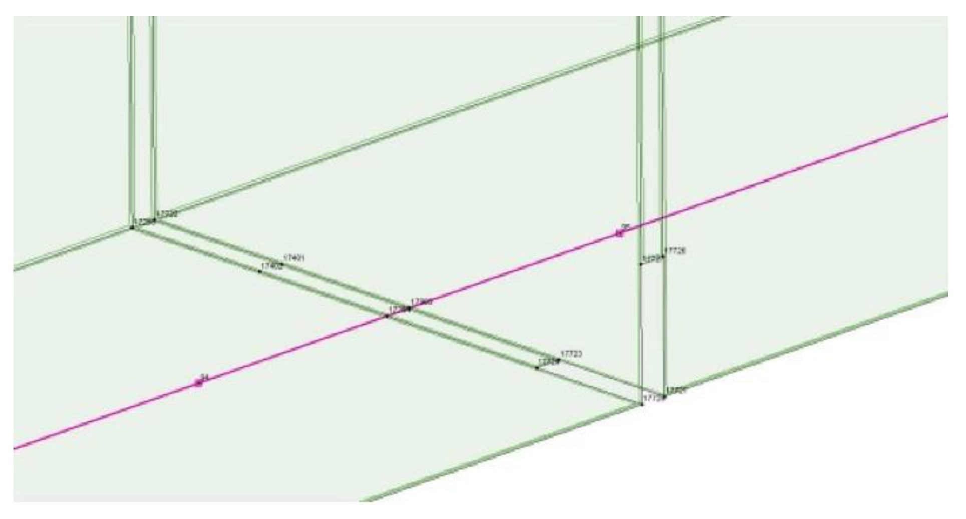
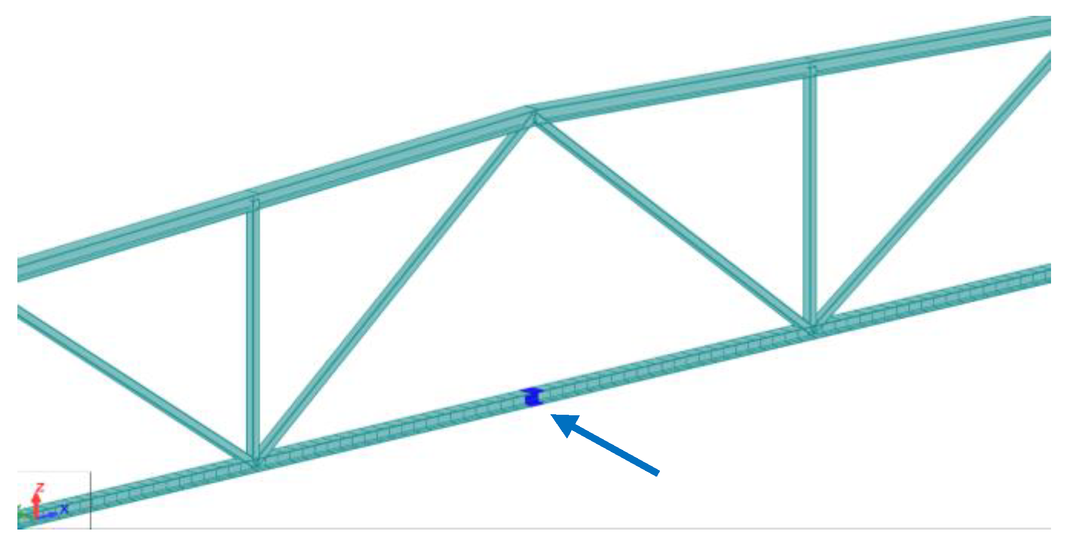
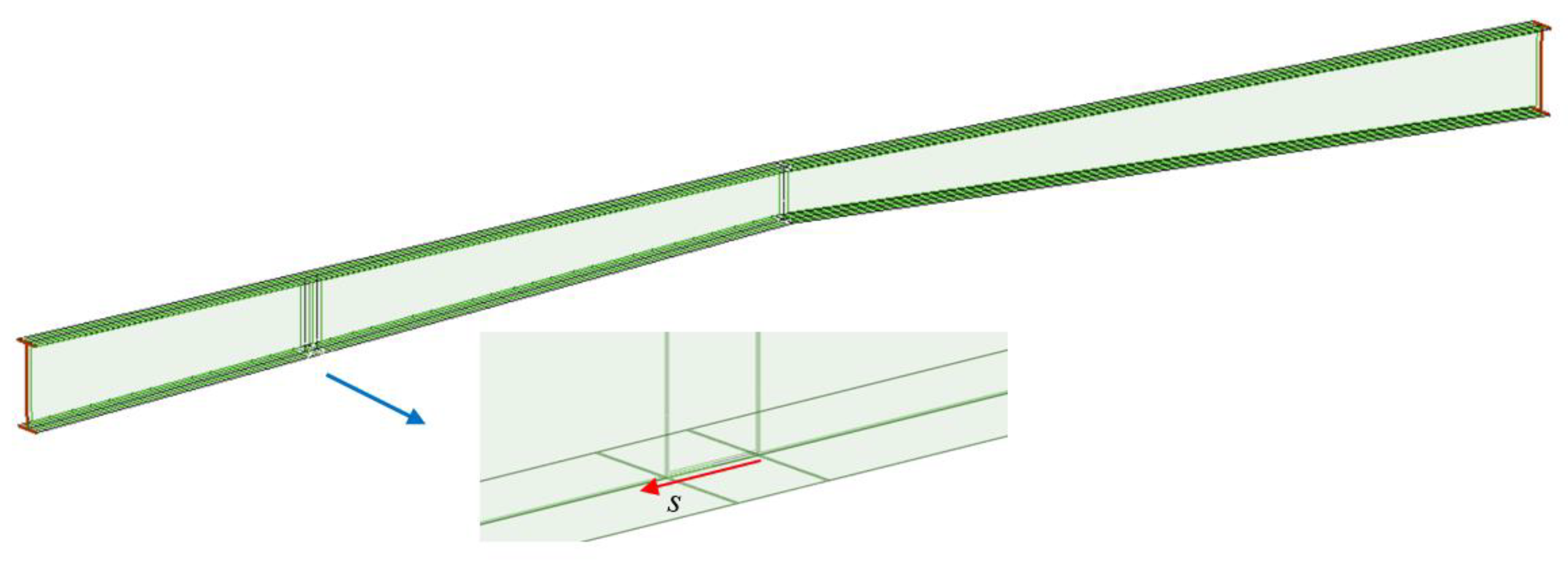
Weaknesses in the structure may be various, for example: a) in the form of reduced cross-section stiffness (Figure 1), b) in the form of a crack at the lower chord of the truss (Figure 2), and c) in the form of scratching at the connection (Figure 3). It is assumed that each of the defects may propagate.

5. Numerical Examples

5.1. The Truss Girder Modeled by Bar Elements

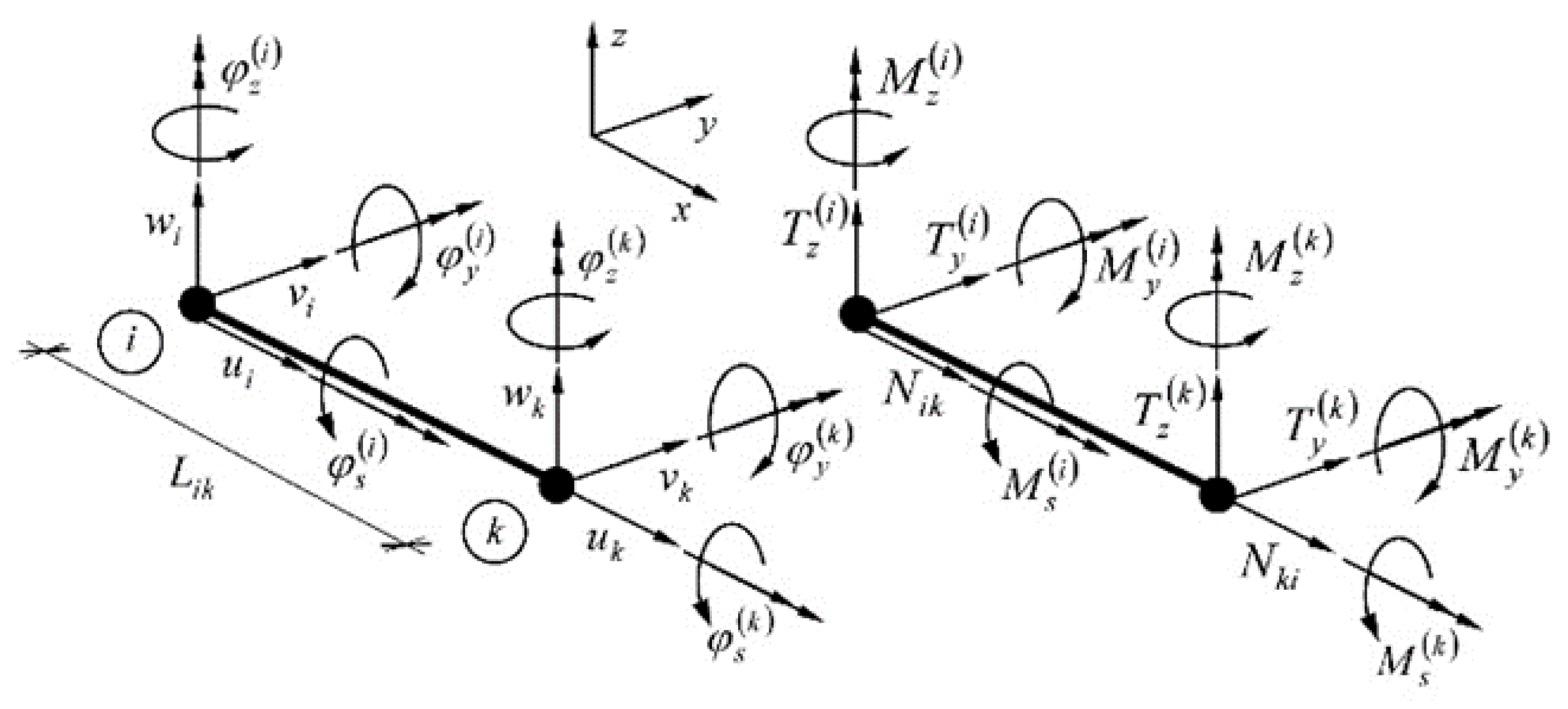
A truss made of steel profiles will be analyzed. The presented structure is an actual and implemented in the reality structural design. To obtain the structural response signal, the numerical analysis using the Finite Element Method (FEM) has been. According to the simplest, bar approach, a two-node spatial bar element has been implemented. This element is shown in Figure 4, where the nodal displacements and the corresponding nodal forces are presented.

The system of equations of the FEM for the whole structure has a classical form:

(5.1) K \cdot q = P,

where K, q, and P are the structural stiffness matrix, structural displacement, and loading vectors.

The material and loading parameters of the structure are presented in Table 1 and Table 2, respectively.

The dimensions of the analyzed single truss girder (assumed with the introduced weakening of the cross-sections) are shown in Figure 5. The number finite elements is 155.

5.1.1. Direct DWT Application

The structural response signal has been analyzed and transformed using DWT procedures. The place of the introduced damage is visible in Figure 6. The weakening was mimicked in the form of a reduction in the value of the elastic Young's modulus along the entire finite element located in the symmetry axis of the truss girder.

The Young modulus E varies regularly from 126 GPa to its reference value E₀ = 210 GPa according to the relation

E = δ \cdot E_{0}

. These relationships are provided in Table 3.

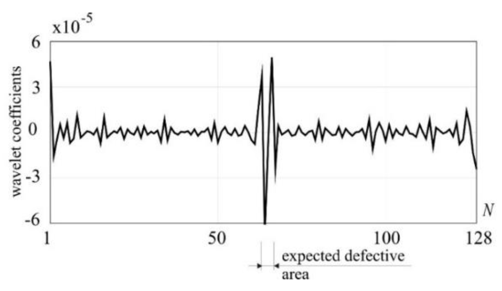
The vertical displacements of the lower chord and the rotation angles of the cross-sections at the FEM nodal points have been measured. The results of DWT transformation of the signal in the form of difference between vertical displacements obtained from defective and undamaged structures are presented in Figure 7. The damage was assumed as 20% of Young's modulus value, namely step 4 of the analysis (see Table 3). It is visible that the evident peak properly indicates the presence and location of the weakened element.

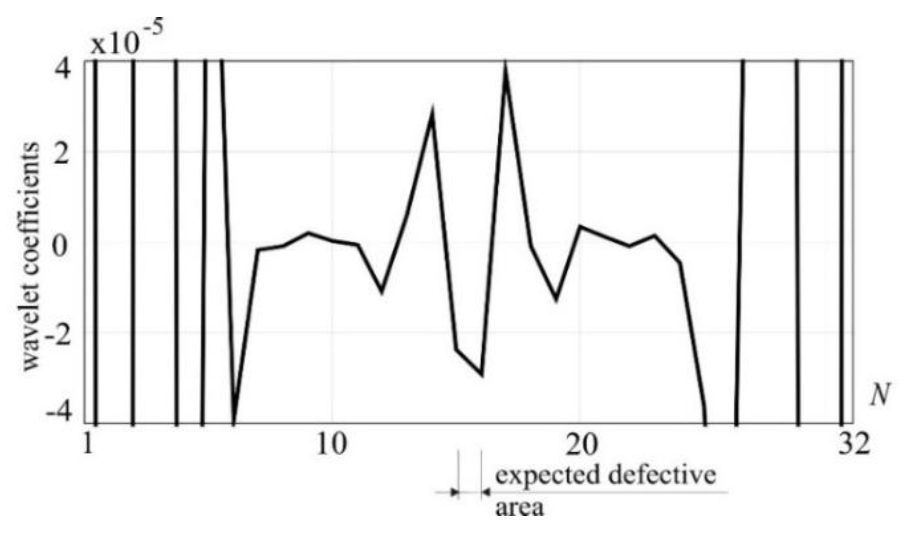
Sufficient transformation accuracy can be observed already at 32 numbers of measurements (Figure 8) for the same intensity of damage, using only the signal from the defective structure.

5.1.2. Direct DWT Application

As part of this example, an initial random analysis of the solution will be performed. To begin with, it was assumed that Young's modulus would play the role of a random variable. The values of this parameter change according to the change in the non-dimensional coefficient δ and together with the corresponding displacements measured at the node placed adjacent to the section of the lower chord where Young's modulus changes are listed in Table 4. The number of trials for the MCS approach is 100000.

The curve fitting according to the LSM procedure is given as the polynomial of the third-degree

(5.2) w (E) = 3.53279132632622 - 0.00110581831515918 \cdot E +

+ 4.49026891793334 \cdot 10^{- 6} \cdot E^{2} + 6.57599837331859 \cdot 1 0^{- 9} \cdot E^{3} .

The expected value

E (E)

coefficient of variation

α (E)

, skewness

β (E)

, and kurtosis

κ (E)

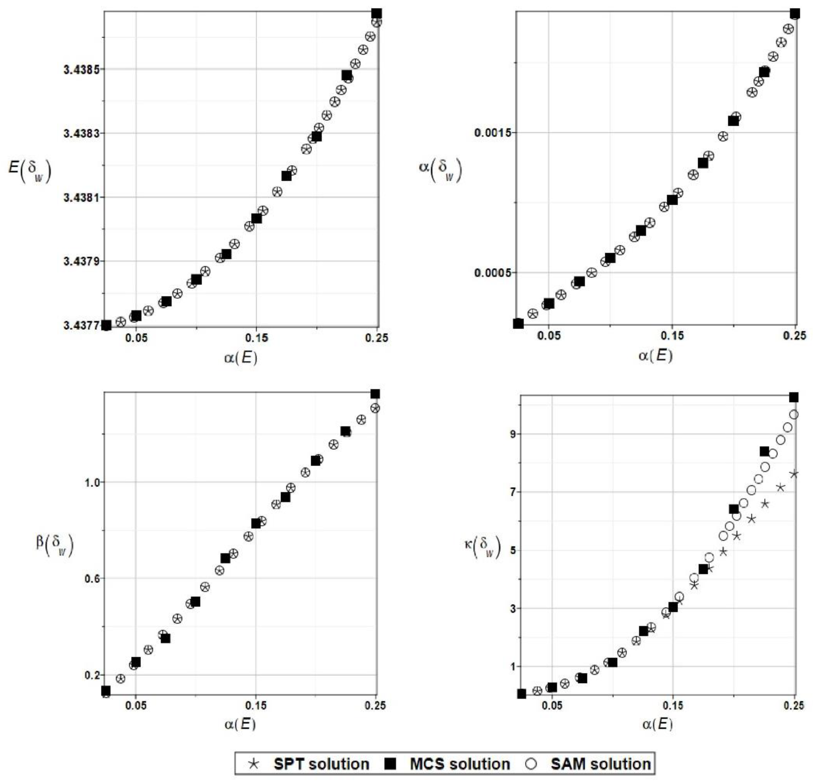
have been presented all in turn in Figure 9 as the functions of the input random modulus coefficient of variation. It is seen that randomization of this parameter causes negligible uncertainty of the selected displacement, so it is expected that higher order statistics diverge from 0 for increasing coefficient of variation. The resulting PDF of the given displacement is remarkably different from the Gaussian distribution curve. Nevertheless, a coincidence of all three probabilistic methods is almost perfect in each case, so that they can be used alternatively depending upon the computer power and software availability.

5.2. The Truss Girder Modeled by Shell Elements

In this example, the shell model of a truss was used. The single truss girder shown in Figure 10 is analyzed. The height of the truss is 2 m, and the span is 24 m. The upper and lower chords are made of steel hot-rolled profiles, i.e., thin-walled square hollow sections SHS 140×140×5 mm and SHS 120×120×4 mm. The diagonals are made of a SHS 90×90×5 mm, SHS 60×60×5 mm and SHS 50×50×5 mm. The most unfavorable combination of loads was selected for analysis. As in the previous example, the set of permanent and varying loads acting were included. Typical four-node finite elements with five degrees of freedom per node (with two in-plane translational displacements, translational displacement perpendicular to the plane, and two independent slopes) will be applied. The analysis by applying typical shell elements will also be considered to estimate the structure's response to a propagating crack. The number of finite elements is 36354.

Figure 10. Analysed truss girder with location of the damage of cross-section.

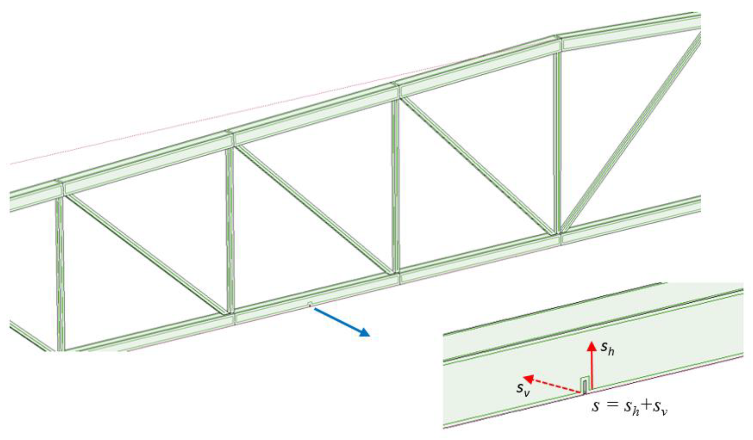
Figure 11. The crack at the lower chord of the truss and line with discrete points to record the data.

5.2.1. Direct DWT Application

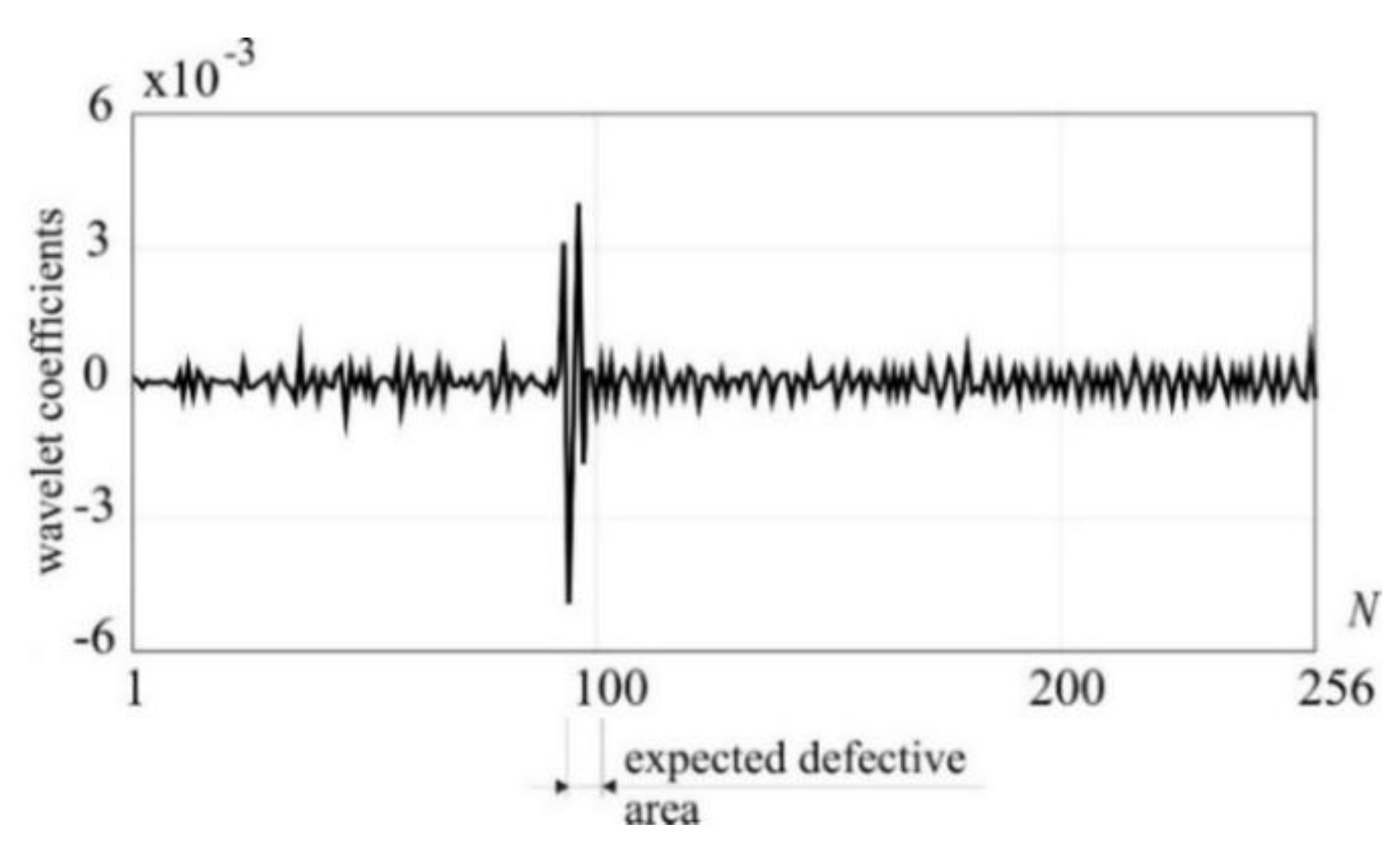
In this example the damage will occur as a crack propagating a) vertically and b) horizontally in the lower chord of the truss structure. For the DWT the signal of vertical displacement measured in discrete points of the lower chord has been taken into consideration. The results of the conducted signal decomposition for step 4, namely the intensity of the crack 4.2 mm in both directions are presented in Figure 12 and Figure 13. The defect was properly localized (high peak) both when analyzing the difference of the signals from the damaged and undamaged structure (Figure 12), as well as only the signal from the damaged truss with a significant reduction of measurement points (see Figure 13).

A sufficient transformation accuracy can be observed already at 32 numbers of measurements (cf. Figure 13).

5.2.2. Random Analysis

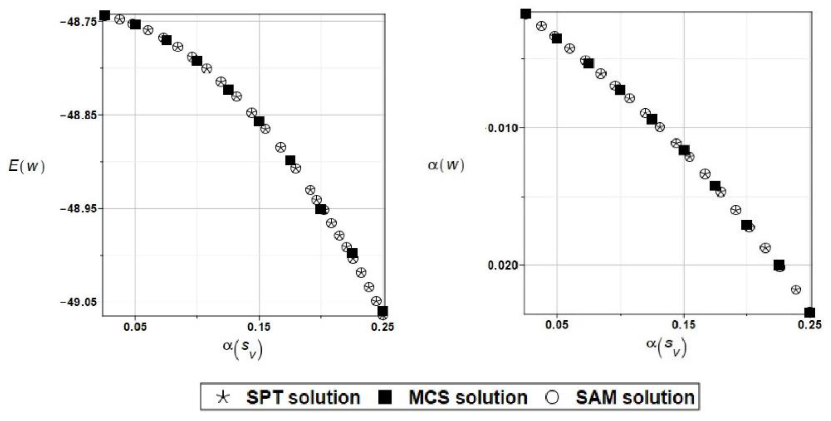
In this example the damage will occur as a crack propagating in a vertical direction and the damage occurs between the nodes indicated in Figure 11. Similarly as above, the response curve fitting is needed and created using eleven discrete points steps. The relationships between the damage propagation coordinate and the vertical displacement at a selected point of the girder are shown in Table 5.

For vertical crack propagation, similarly as in the previous example the curve fitting is given as the polynomial of the third degree, where the polynomial was determined for the axis of vertical displacements directed upwards (according to the coordinate system used in the calculation program)

(5.3) w (s_{v}) = - 46.1403543123539 - 0.953728308728512 \cdot s_{v} + + 0.186485042735074 \cdot s_{v}^{2} - 0.0154060188782405 \cdot s_{v}^{3} .

The results obtained for the first two probabilistic moments are shown in Figure 14 and a very good convergence of the values of the two first probabilistic moments obtained using the SAM, SPT, and MCS methods can be observed even for higher values of the input coefficient of variation, which never happen in engineering practice. The negligible character of this uncertainty type is quite clear from the right graph below.

5.2.3. Uncertainty in the Given Wavelet Coefficients

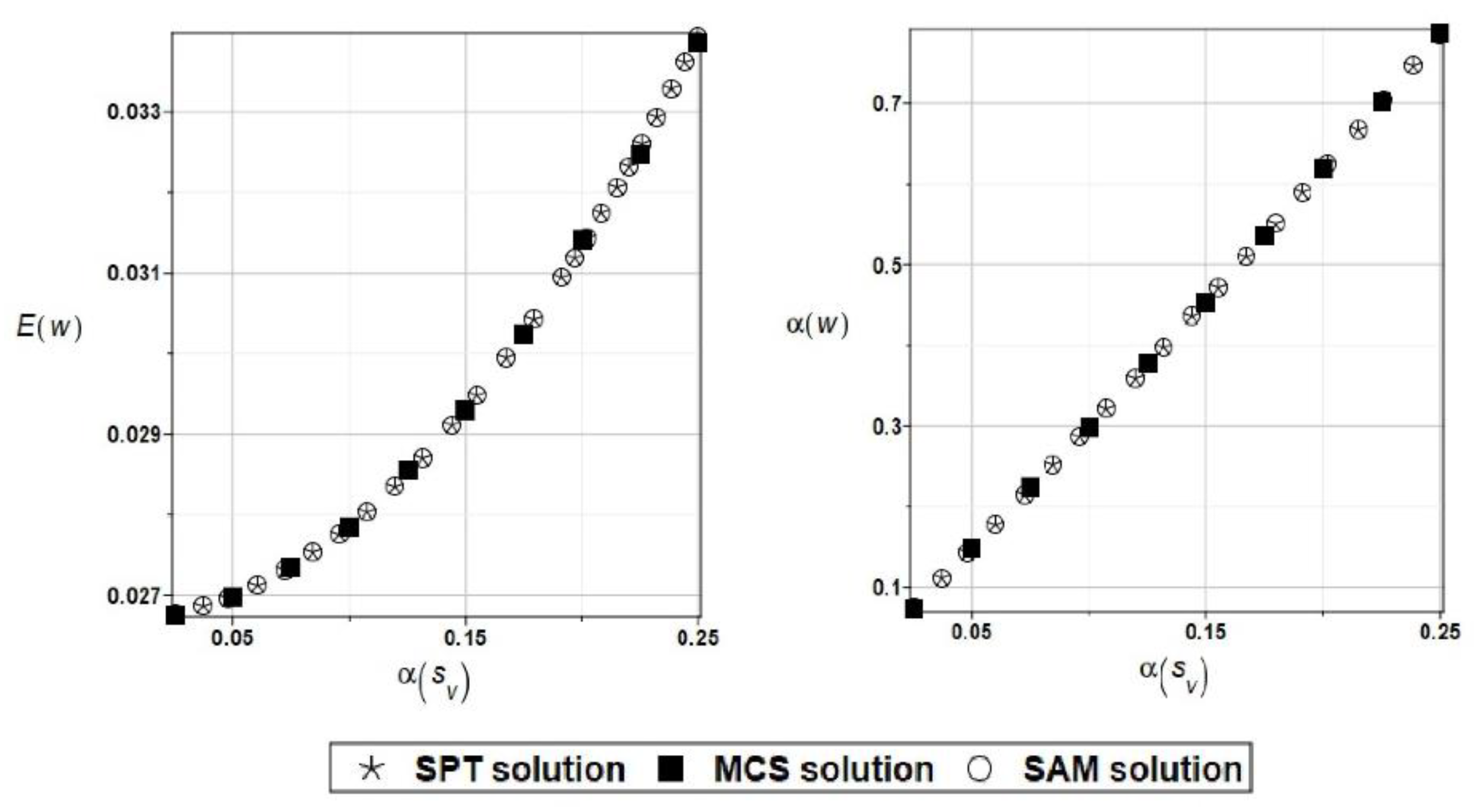
Finally, the value of the vertical displacement expressed by the wavelet function determined at a point belonging to the damaged area was also randomized. Similarly, as above, the curve fitting is given as the polynomial of the third-degree polynomial

(5.4) w (s_{v}) = - 0.0356604195804185 + 0.02206824009324 \cdot s_{v} - - 0.00419800569800572 \cdot s_{v}^{2} + 0.000346358888025557 \cdot s_{v}^{3}

The obtained results for the first two probability moments are shown in Figure 15. Also here, a very good convergence of the results obtained using three different random methods was observed. The most important research finding is that these wavelet coefficients are extremely important in this analysis, because the output uncertainty in the vertical displacements are three times larger than the corresponding input randomness.

5.3. The I-Section Steel Girder Modeled by Shell Finite Elements

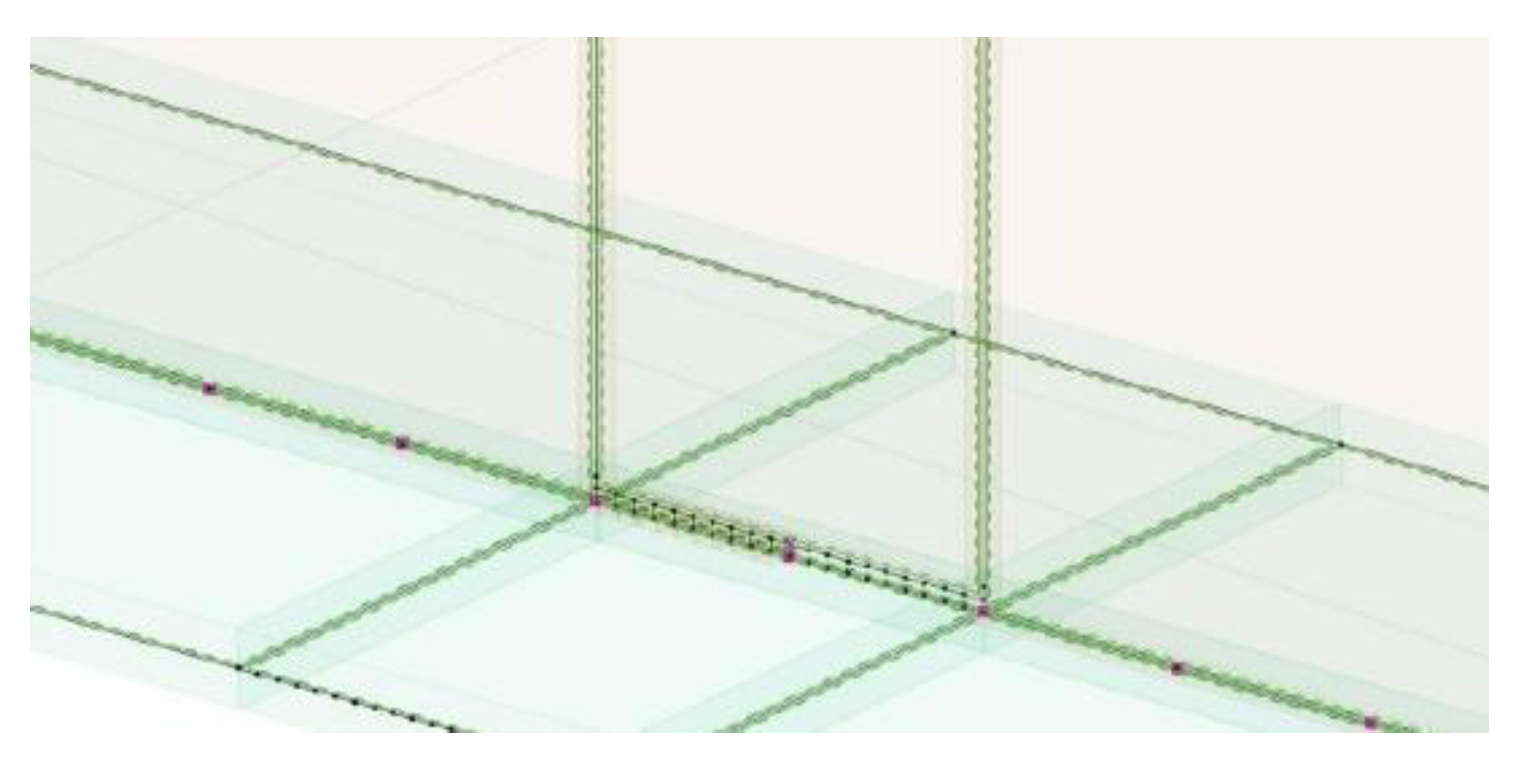
In the following analysis, the steel girder with a weakening in the form of scratching was analyzed. The single steel girder with the location of the damage in Figure 16 is presented. The height of the girder is variable (from 0.6 m to 1.0 m), and the span is 24 m. As in previous examples, the most unfavorable combination of loads was selected. The number finite shell elements is 13013.

5.3.1. Random Analysis

In this case, the crack will develop horizontally. Damage occurs between nodes indicated in Figure 17. Similar to the previous example the response curve fitting is created based on eleven discrete points steps. The relationships between the damage propagation coordinate and the horizontal displacement at a selected point of the girder are shown in Table 6.

For horizontal crack propagation, the same as before, the curve fitting is given as the polynomial of the third degree, where the polynomial was determined for the axis of vertical displacements directed upwards (according to the coordinate system used in the calculation program).

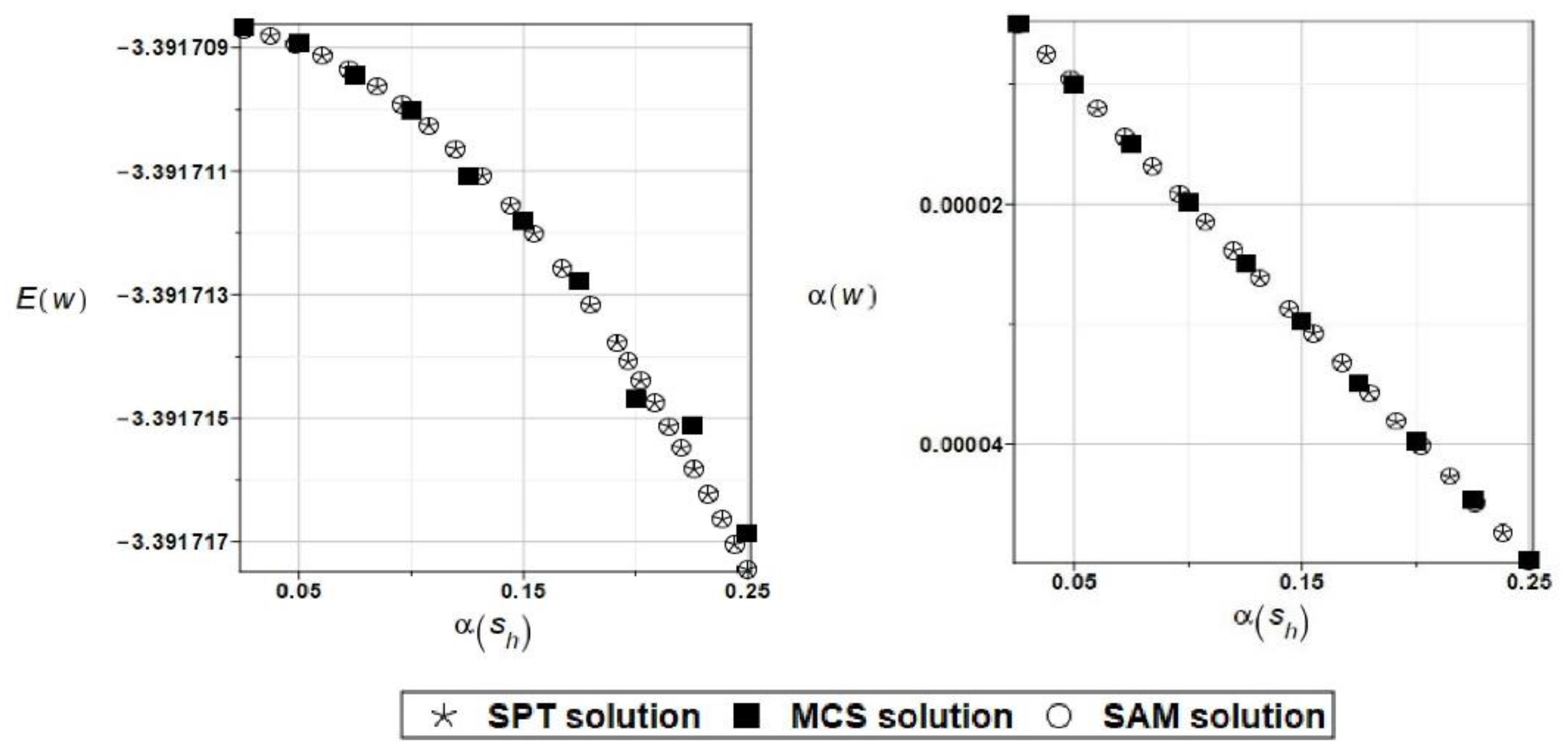
(5.5) w (s_{h}) = - 3.39119539627037 - 0.00350497611230616 \cdot s_{h} - - 0.0232150526299201 \cdot s_{h}^{2} + 0.0257259004967464 \cdot s_{h}^{3}

The results of calculations for the first two probability moments are shown in Figure 18.

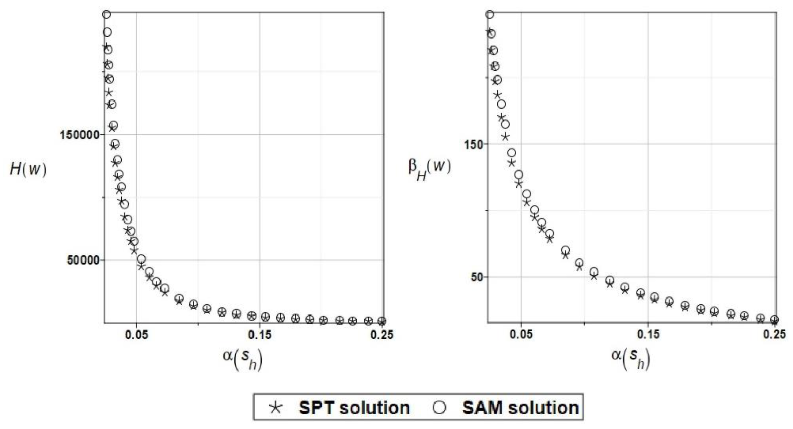
A very good convergence of the results obtained using the three random methods can be observed for the first three random moments. During random analysis, the probabilistic entropy may be determined, and based on it, a measure of reliability according to the Bhattacharyya proposition [23,24]. These relations as a function of the input coefficient of variance are shown in Figure 19. Typically for the First Order Reliability Method (FORM) analysis, the reliability index numerical values exponentially decay while increasing of the input uncertainty level of the horizontal damage parameter. It is also seen that the results coming from both stochastic perturbation method and the semi-analytical approach are almost equal to each other, which confirms wide applicability of the generalized iterative perturbation method, whose application is demonstrated in this work. Additionally, one notices that the SPT computations return slightly smaller numerical values, which means that they are less favourable while assessing reliability of the truss; therefore, they would be recommended.

6. Concluding Remarks

This paper presents an analysis of structural damage detection using discrete wavelet transform. The structural response signal is subjected to wavelet transformation in the form of, for example, a discrete set of displacements determined at selected points of the structure – in this case, finite element nodes. Application of 1-D Discrete Wavelet Transform (DWT) allowed for clear localization of existing damage. The set of Daubechies type wavelet functions has been used. The basis for obtaining the structure's response signal is a numerical analysis using the FEM approach. The present work has also been extended to the additional studies covering the application of three probabilistic approaches: the semi-analytical (SAM), perturbation-based (SPT), and Monte-Carlo simulation technique (MCS) and also to define and calculate reliability measures based on the relative entropy H according to the Bhattacharyya theory. This approach allows you to obtain a solution in a certain random interval determined by the coefficient of variation of the argument. A very good convergence of the results obtained by these three methods can be observed. The reliability measures show that their values are decreasing deeply with an increasing value of the coefficient of variance of the random variable. The need to use a large number of trials in Monte Carlo simulation makes this method the most time-consuming one, but an increase in the precision for higher-order statistics is relatively small and not necessary for most engineering analyses. The semi-analytical approach seems to be the most adequate due to its simplicity and reasonable computation time for random numerical simulations of structural mechanics tasks. Taking into account particular numerical values of the resulting uncertainties in the Serviceability Limit State (SLS) it has been demonstrated that the vertical crack is the decisive parameter for the given truss reliability as its CoV reaches maximum value for the same input statistical scattering of all tested parameters.

Funding

Financial support of the Institute of Structural Analysis under grant 0411/SBAD/0008 is highly appreciated. This work contains also the results obtained in the framework of the research grant OPUS no. 2021/41/B/ST8/02432 entitled “Probabilistic entropy in engineering computations” sponsored by the National Science Center in Cracow, Poland, 2022–2025.

References

Mróz, Z.; Garstecki, A. Optimal loading conditions in design and identification of structures. Part 1: Discrete formulation. Struct. Multidiscip. Optim. 2005, 29, 1–18. [Google Scholar] [CrossRef]
Burczyński, T.; Kuś, W.; Długosz, A.; Orantek, P. Optimization and defect identification using distributed evolutionary algorithms. Eng. Appl. Artif. Intell. 2004, 17, 337–344. [Google Scholar] [CrossRef]
M. Rucka, K. Wilde, “Neuro-wavelet damage detection technique in beam, plate and shell structures with experimental validation”, Journal of Theoretical and Applied Mechanics, vol. 48, no. 3, pp. 579-604, 2010.
Kamiński, M. Homogenization-based finite element analysis of unidirectional composites by classical and multiresolution techniques. Comput. Methods Appl. Mech. Eng. 2005, 194, 2147–2173. [Google Scholar] [CrossRef]
Knitter-Piątkowska, M. Guminiak, and M. Przychodzki, “Application of Discrete Wavelet Transformation to defect detection in truss structures with rigidly connected bars”, Engineering Transactions, vol. 64, no. 2, pp. 157-170. 2016. [Google Scholar] [CrossRef]
Knitter-Piątkowska, A.; Dobrzycki, A. Application of Wavelet Transform to Damage Identification in the Steel Structure Elements. Appl. Sci. 2020, 10, 8198. [Google Scholar] [CrossRef]
Ziopaja, K.; Pozorski, Z.; Garstecki, A. Damage detection using thermal experiments and wavelet transformation. Inverse Probl. Sci. Eng. 2011, 19, 127–153. [Google Scholar] [CrossRef]
Hanteh, M.; Rezaifar, O.; Gholhaki, M. Selecting the appropriate wavelet function in the damage detection of precast full panel building based on experimental results and wavelet analysis. J. Civ. Struct. Heal. Monit. 2021, 11, 1013–1036. [Google Scholar] [CrossRef]
Mariak, A.; Wilde, K. Multipoint Ultrasonic Diagnostics System Of Prestressed T-Beams. Arch. Civ. Eng. 2014, 60, 475–492. [Google Scholar] [CrossRef]
Wang, X.; Tang, J. Structural damage detection using a magnetic impedance approach with circuitry integration. Smart Materials and Structures 2008, 20, 035022. [Google Scholar] [CrossRef]
Chen, T.; Tian, G.Y.; Sophian, A.; Que, P.W. Feature extraction and selection for defect classification of pulsed eddy current NDT. NDT E Int. 2008, 41, 467–476. [Google Scholar] [CrossRef]
Skłodowski, R.; Drdácký, M.; Skłodowski, M. Identifying subsurface detachment defects by acoustic tracing. NDT E Int. 2013, 56, 56–64. [Google Scholar] [CrossRef]
Wójcik, B.; Żarski, M. The measurements of surface defect area with an RGB-D camera for a BIM-backed bridge inspection. Bull. Pol. Acad. Sci. Tech. Sci. 2021, 69, 137123–137123. [Google Scholar] [CrossRef]
Skowron, M. Application of deep learning neural networks for the diagnosis of electrical damage to the induction motor using the axial flux. Bull. Pol. Acad. Sci. Tech. Sci. 2020, 68, 1031–1038. [Google Scholar] [CrossRef]
Lu, W.; Dong, J.; Pan, Y.; Li, G.; Guo, J. Damage identification of bridge structure model based on empirical mode decomposition algorithm and Autoregressive Integrated Moving Average procedure. Arch. Civ. Eng. 2022, 68, 653–667. [Google Scholar] [CrossRef]
Kamiński, M. The Stochastic Perturbation Method for Computational Mechanics. Chichester: Wiley, 2013.
Kamiński, M. On the dual iterative stochastic perturbation-based finite element method in solid mechanics with Gaussian uncertainties. Int. J. Numer. Methods Eng. 2015, 104, 1038–1060. [Google Scholar] [CrossRef]
Chowdhury, M.S.; Song, C.; Gao, W. Probabilistic fracture mechanics with uncertainty in crack size and orientation using the scaled boundary finite element method. Comput. Struct. 2014, 137, 93–103. [Google Scholar] [CrossRef]
Zhang, N.; Yao, L.; Jiang, G. A coupled finite element-least squares point interpolation/boundary element method for a structure-acoustic system with stochastic perturbation method. Eng. Anal. Bound. Elements 2020, 119, 83–94. [Google Scholar] [CrossRef]
R. Bredow, M. Kamiński, “Dynamic analysis of steel mast under some environmental uncertainties”, Lightweight Structures in Civil Engineering, Contemporary Problems. Łódź: Łódź University of Technology Press, 2021, pp. 171-180.
Daubechies, Ten lectures on wavelets. Philadelphia: Society for Industrial and Applied Mathematics, 1992.
Mallat, S. A Wavelet Tour of Signal Processing; Academic Press: San Diego, CA, USA, 1999. [Google Scholar]
Bhattacharyya, “On a measure of divergence between two multinomial populations”, Indian Journal of Statistics, vol. 7, 401–406, 1946. [CrossRef]
Xiang, Y.; Liu, Y. Application of inverse first-order reliability method for probabilistic fatigue life prediction. Probabilistic Eng. Mech. 2011, 26, 148–156. [Google Scholar] [CrossRef]
G. Rakowski, Z. Kacprzyk, The Finite Element Method in structural mechanics, Warsaw University of Technology Publishing House, 2005.

Figure 1. Weakening in the form of a reduction in stiffness (loss) on the cross-section.

Figure 2. Weakening in the form of a crack at the lower chord of the truss.

Figure 3. Weakening in the form of a scratching at the connection.

Figure 4. The two-node finite element used for the description analyzed truss [25].

Figure 5. Truss girder subjected to damage detection analysis.

Figure 6. Analysed truss girder with introduced weakened element.

Figure 7. 1-D DWT of vertical displacements, step 4–0, Daubechies 6, detail 1, N – numbers of measurements.

Figure 8. 1-D DWT of vertical displacements, step 4, Daubechies 8, detail 1, N – numbers of measurements.

Figure 9. Expected value, coefficient of variation, skewness, and kurtosis of the displacement at selected truss node while randomizing steel Young modulus.

Figure 12. 1-D DWT of vertical displacements, step 4–0, crack, Daubechies 6, detail 1, N – numbers of measurements.

Figure 13. 1-D DWT of vertical displacements, step 4, Daubechies 8, detail 1, N – numbers of measurements.

Figure 14. Expected value and coefficient of variation of the vertical displacement at selected truss node while randomizing vertical crack propagation.

Figure 15. Expected value and coefficient of variation of the vertical displacement transformed by DWT at selected truss node while randomizing vertical crack propagation.

Figure 16. Analyzed girder with location of the damage of cross-section.

Figure 17. Weakening in the form of a crack propagation.

Figure 18. Expected value and coefficient of variation of the horizontal displacement at selected truss node while randomizing vertical crack propagation.

Figure 19. The probabilistic relative entropy safety measure for the random distribution of the horizontal damage distribution.

Table 1. Material data of the analysed truss.

Data	Steel	Cross-section
Lowe chord	S235	HEA120
Upper chord	S235	HEA140
Cross rod	S235	RK 70×70×4

Table 2. Loading data of the analysed truss.

Loading	Deadweight	Constant	Variable	Snow	Wing
Lowe chord	Standard	2.1	2.4	4.32	0.9

Table 3. Assumed variability of Young's modulus.

Step	0 (ref.)	1	2	3	4	5	6	7	8
δ	1	0.95	0.9	0.85	0.8	0.75	0.7	0.65	0.6
E [GPa]	210.0	199.5	189.0	178.5	168.0	157.5	147.0	136.5	126.0

Table 4. Assumed variability of Young's modulus.

δ	0.75	0.8	0.85	0.9	0.95	1.0
E [GPa]	157.5	168.0	178.5	189.0	199.5	210.0
w(E) [mm]	3.44429	3.44261	3.44113	3.43981	3.43863	3.43757
δ	1.05	1.1	1.15	1.2	1.25	–
E [GPa]	220.5	231.0	241.5	252.0	262.5	–
w(E) [mm]	3.43660	3.43573	3.43493	3.4342	3.43352	–

Table 5. Vertical crack propagation; vertical coordinate and the vertical displacement.

s_v [mm]	3.6	4.2	4.8	5.4	6.0	6.6
w(s_v) [mm]	47.892	47.982	48.105	48.287	48.484	48.743
s_v [mm]	7.2	7.8	8.4	9.0	9.6	–
w(s_v) [mm]	49.098	49.57	50.103	50.815	51.765	–

Table 6. Damage propagation. Horizontal coordinate and the horizontal displacement.

s_h [mm]	4.70	5.64	6.58	7.52	8.46	9.40
w(s_h) [mm]	3.39141	3.39146	3.39152	3.39158	3.39164	3.39171
s_h [mm]	10.34	11.28	12.22	13.16	14.10	–
w(s_h) [mm]	3.39178	3.39185	3.39192	3.392	3.39208	–

Disclaimer/Publisher’s Note: The statements, opinions and data contained in all publications are solely those of the individual author(s) and contributor(s) and not of MDPI and/or the editor(s). MDPI and/or the editor(s) disclaim responsibility for any injury to people or property resulting from any ideas, methods, instructions or products referred to in the content.

© 2024 by the authors. Licensee MDPI, Basel, Switzerland. This article is an open access article distributed under the terms and conditions of the Creative Commons Attribution (CC BY) license (https://creativecommons.org/licenses/by/4.0/).

Copyright: This open access article is published under a Creative Commons CC BY 4.0 license, which permit the free download, distribution, and reuse, provided that the author and preprint are cited in any reuse.

MDPI Initiatives

Important Links

Choose an area of interest and we will send you notifications of new preprints at your preferred frequency.

Disclaimer