Preprint
Article

Time-Delay Dynamic Model and Cost-Effectiveness Analysis of Major Emergent Infectious Diseases with Transportation-Related Infections and Entry-Exit Screening

Altmetrics

Downloads

92

Views

27

Comments

0

A peer-reviewed article of this preprint also exists.

Submitted:

03 June 2024

Posted:

04 June 2024

You are already at the latest version

Alerts
Abstract
We analyze a time-delayed SIQR model that considers the transportation-related infections and entry-exit screening. This model aims to determine the measures for preventing and controlling major emergent infectious diseases and the associated costs. We calculate the basic reproduction number (R0), apply the linearization method, and construct an appropriate Lyapunov function to determine the stability of the disease-free equilibrium in the local and global. We collect COVID-19 infection data from two regions in the United States in 2020 for data fitting, obtain a set of optimal parameter values, and show that the model is suitable for simulating the outbreak and spread of emerging infectious diseases. We find that transportation-related infections increase the basic reproduction number, enhancing the impact on disease spread. Entry-exit screening effectively suppress the spread of disease by reducing the basic reproduction number. Furthermore, we investigate the influence of the incubation period on disease and find that a shorter incubation period results in a shorter duration but a larger scale of infection, and the peaks are reduced. We conduct a sensitivity analysis of the R0 and propose three measures to prevent the spread of new infectious diseases based on the most sensitive parameters: wearing masks, implementing urban closures, and administering medication to sick but not yet hospitalized patients promptly. In the case of COVID-19, we use Pontryagin’s minimum principle to get time-varying control measures to control the spread of the outbreak. Optimal control effectively controls the development and deterioration of the disease. Finally, several control measures are compared through cost-effectiveness analysis, and the results show that wearing masks is the most cost-effective measure. Our study provides some practical guidance for controlling the spread of major emerging infectious diseases.
Keywords: 
Subject: Biology and Life Sciences  -   Life Sciences

1. Introduction

In today’s society, infectious diseases are constantly threatening human health. Therefore, understanding the outbreak mechanism and transmission mode of infectious diseases will help shed light on future prevention and treatment strategies. When the first case of AIDS was covered in America in June 1981, more and more people were infected and even dying of AIDS throughout the 1980s, and there is still a large population of AIDS patients today [1]. In 2003, an outbreak of Severe Acute Respiratory Syndrome (SARS) occurred in Guangdong Province, China, characterized by its high infectivity and rapid disease progression, eventually leading to outbreaks in various regions of China and some cities worldwide [2]. In 2009, a widespread outbreak of H1N1 influenza occurred in the United States and rapidly spread to other countries and regions [3]. In March 2013, H7N9 was first discovered in eastern China [4]. A flare-up of H7N9 avian influenza quickly gained wide attention as new cases and high infection-related death rates were not controlled. At the end of 2019, COVID-19 rapidly swept the world, becoming one of the most serious diseases in human history [5]. An increasing number of sudden infectious diseases are emerging, some of which have become endemic, continuing to harm humans. In contrast, others have evolved into more insidious and harmful viruses through the continuous mutation of viruses.
Infectious disease modeling is a vital field that investigates the transmission routes and factors influencing the spread of emerging infectious diseases. With the rapid development of the global economy and the increasingly convenient means of transportation, population movements and people spreading the virus along the way are recognized as critical factors in disease transmission, which has attracted extensive attention from researchers. Perrin et al. [6] emphasized that the global dissemination of the HIV-1 pandemic fundamentally revolves around travel, implying the significance of travel in disease transmission. Air travel is also considered pivotal in spreading infectious diseases, as discussed by Mangili and Gendreau [7], who explored the potential for disease epidemics associated with air travel. In Beijing, China, Jia et al. [8] conducted a study revealing the impact of population mobility on tuberculosis’s prevalence, further highlighting the role of population mobility in disease transmission. In addition, the study of Chan et al. [9] revealed that person-to-person transmission of the novel coronavirus is possible within households, hospitals, and between cities. To better understand and predict transportation-related disease spread, Cui et al. [10] proposed an epidemiological model that describes this transmission mode. Similarly, Liu et al. [11] developed an SIQS infectious disease model incorporating transportation and entry screening, demonstrating the effectiveness of entry screening in mitigating transportation-related disease transmission. Many similar models of infectious diseases spread between two regions [12,13,14,15,16]. In addition to considering patch models for two regions, many authors also consider patch models for multiple regions. In 2003, Arino et al. [17] proposed a model for the spread of disease in a population of individuals traveling between n cities. The results show that R 0 is a threshold, when R 0 < 1 , the disease disappears, and when R 0 > 1 , the disease reaches epidemic levels in all connected cities. Gao and Ruan [18] proposed a model with multiple patches to study how population movement affects the spread of malaria. Their results showed that travel between areas contributed to the spread of the disease in both regions. However, if travel rates continue to increase, the disease might disappear again in both areas. Sun et al. [19] established a patch model reflecting the population flow between Hubei and other regions. They estimate the epidemic situation in Hubei based on the daily reported epidemic data from Hubei and other regions, as well as the data on the population flow between Hubei and other regions. Zhang et al. [20] established a multi-patch model of HIV/AIDS with heterosexual transmission. The results indicate that if the disease vanishes in one region and spreads in another, it can spread or disappear in both regions depending on the individual mobility patterns.
Prosper et al. [21] proposed an optimal control model for malaria and find that the effectiveness of vaccination programs at the population level can be improved by actively seeking out and treating asymptomatic infections. Kang et al. [22] proposed a delayed avian influenza model incorporating slaughtering conditions. Their study indicates that optimal control, achieved by slaughtering susceptible (infected) avians and educating susceptible populations, can effectively minimize the number of infections in poultries and mankind. Moreover, the cost of implementing these control strategies can be minimized. Song et al. [23] studied the impact of delayed vaccination and isolation on COVID-19 transmission and conclude that the best isolation rate minimizes the total number of infections and expenditure on disease control. Singh et al. [24] have found that measures such as social distancing, lockdowns, and wearing masks can reduce the spread of the disease. These studies and models provide valuable insights and guidance for our in-depth understanding of the impact of population movements and traffic factors on disease transmission and how to control disease effectively.
For diseases such as tuberculosis, hepatitis A, hepatitis B, and influenza, the process of infection is unique because susceptible individuals do not immediately become ill after infection. Instead, they undergo an incubative period, where the pathogens replicate and spread within the host without showing noticeable symptoms. With this factor in mind, many researchers have proposed infectious disease models with delayed incubative periods in mathematical modeling and conducted extensive studies in this field [25,26,27,28,29,30,31,32]. Although many infectious disease models take into account the presence of incubative periods, we also need to be aware of the limitations of these models. The exact length of the incubative periods, variations in infectiousness, and interactions between individuals can all introduce uncertainty into the models. Therefore, further research is still needed to validate and improve the accuracy of these models by incorporating actual data and conducting field investigations. So it is also extremely interesting that we discuss the effect of time delay on measures of time-varying control.
Major emerging infectious diseases differ from normalized infectious diseases, as they have uncertainty, stronger stealthiness, more destructive power, and more severe harm to society and the economy. Therefore, studying the characteristics of sudden outbreaks and epidemics of infectious diseases can help reduce the harm of infectious diseases. From the above revelation, relatively limited studies use actual data to explore transportation-related infections between two regions and how to control this spread effectively. The rest of this paper is organized as follows. In the next section, we establish an SIQR time-delayed infectious disease model for emerging infectious diseases that considers transportation-related infection and entry-exit screening. We count the basic reproduction number and demonstrate that the endemic equilibrium is sole, the global asymptotic stability of the disease-free equilibrium, and the persistence of the model (1). In the section 3, we simulate the model using actual data from two regions in the USA and sensitivity analysis of R 0 . We investigate optimal control strategies in the section 4, and the cost-effectiveness analysis results are presented in the section 5. Discussions and conclusions are provided in the last two sections.

2. Time-Delay Model with Entry-Exit Screening and Transportation-Related Infections

2.1. Model Formulation

We posit that the two regions are identical, signifying that the population parameters in each region are comparable. This assumption holds merit when both regions exhibit similar population density levels, living conditions, economic factors, healthcare services, and disease transmission probabilities. We designate θ e and θ d , where 0 < θ e , θ d < 1 , which represent the probabilities of successfully detecting an infected person for entry screening and exit screening, respectively. Moreover, we assume that susceptible individuals will not be mistakenly identified as infected. Once infected individuals are detected, they undergo isolation in designated hospitals for treatment. However, border screening differs from quarantine or isolation, as it explicitly addresses infections related to transportation. The former can thwart the spread of diseases from one region to another, while the latter effectively prevents the localized spread of diseases within a region. Nevertheless, in the absence of transportation-related infections or under extreme scenarios where θ d = 1 or θ e = 1 , border screening equates to isolating or quarantining a certain proportion of infected individuals. We propose a hypothesis similar to that of many other authors [10,11,33].
After the patients recover, they have a temporary immunity to ensure they do not relapse for a certain period. We consider the disease’s incubation period, leading to the following time-delayed infectious disease model. In the model, τ stands for the disease’s incubation period, and e μ τ S i ( t τ ) I i ( t τ ) , ( i = 1 , 2 ) denotes how many people have not died at time t after been infected at time t τ . e μ τ is the probability that the infected human survives to time t (with the death rate μ ). We consider that e μ τ approaches 1, 1 e μ τ approaches 0, so we ignore 1 e μ τ in our model. The model appears as follows:
d S 1 d t = Λ β S 1 I 1 α S 1 + α S 2 1 θ d γ α S 2 I 2 μ S 1 , d I 1 d t = β S 1 ( t τ ) I 1 ( t τ ) e μ τ + 1 θ e 1 θ d γ α S 2 ( t τ ) I 2 ( t τ ) e μ τ + 1 θ e 1 θ d α I 2 ( b + d + α ) I 1 , d Q 1 d t = θ e 1 θ d γ α S 2 I 2 + θ d α I 1 + θ e 1 θ d α I 2 ( c + f ) Q 1 , d R 1 d t = f Q 1 + d I 1 α R 1 + α R 2 μ R 1 , d S 2 d t = Λ β S 2 I 2 α S 2 + α S 1 1 θ d γ α S 1 I 1 μ S 2 , d I 2 d t = β S 2 ( t τ ) I 2 ( t τ ) e μ τ + 1 θ e 1 θ d γ α S 1 ( t τ ) I 1 ( t τ ) e μ τ + 1 θ e 1 θ d α I 1 ( b + d + α ) I 2 , d Q 2 d t = θ e 1 θ d γ α S 1 I 1 + θ d α I 2 + θ e 1 θ d α I 1 ( c + f ) Q 2 , d R 2 d t = f Q 2 + d I 2 α R 2 + α R 1 μ R 2 .
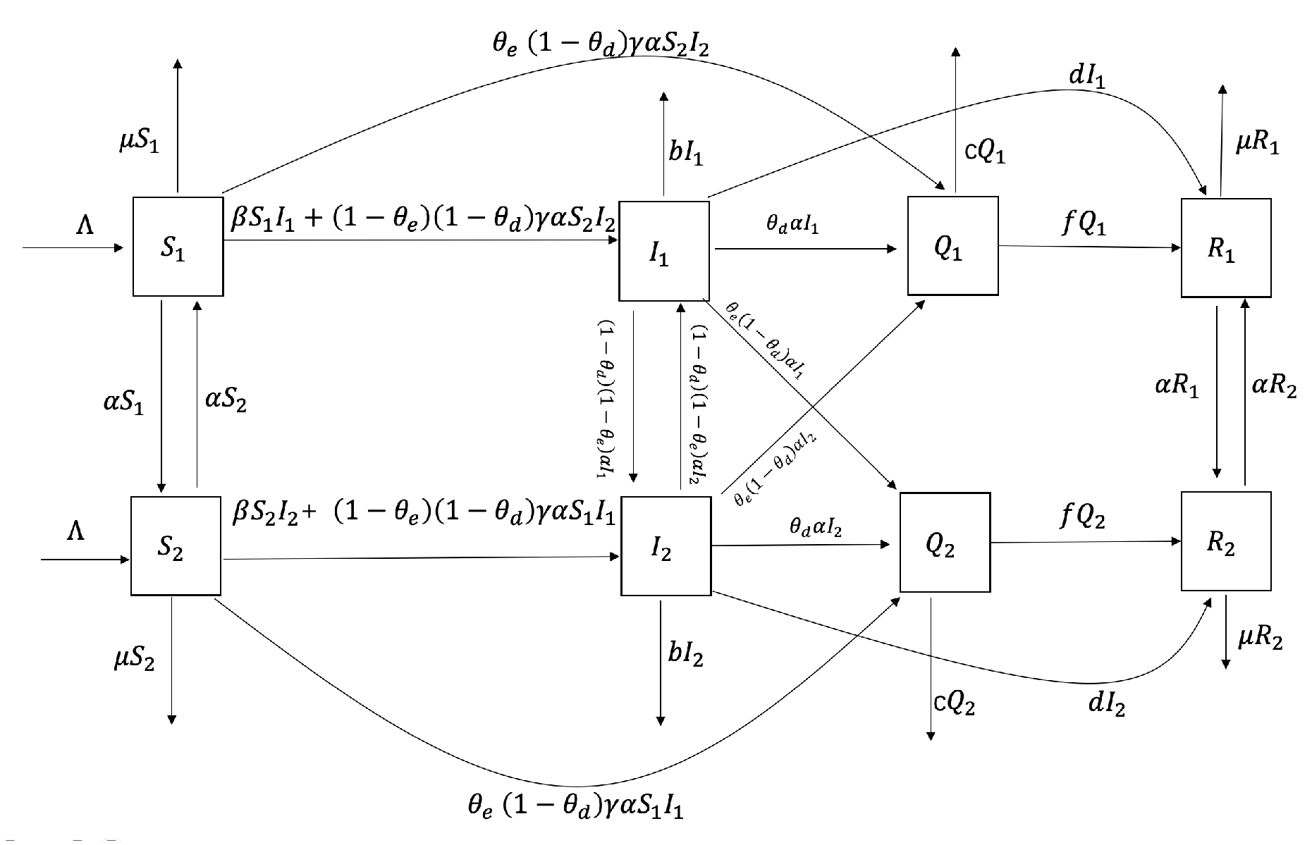
Here S i and I i ( i = 1 , 2 ) represent the number of susceptible and infected individuals in region i (we use the results of the entry-exit screening as a criterion for whether the population has the disease), Q i ( i = 1 , 2 ) denotes such isolated infected individuals in each region, R i ( i = 1 , 2 ) represents the number of the removed individuals in region i. Table 1 lists the biological interpretations of all parameters. The per capita mortality rate for infected individuals is b, and c means the average death rate of isolated infected individuals. Because not only natural mortality but disease-caused mortality are included in it, we have μ b , μ c . In model (1), rate of disease (that is, how many new infection cases are added within a unit of time) β S i I i , i = 1 , 2 , within city i. The susceptible and infected individuals in each i leave for city j ( i j , i , j = 1 , 2 ) at a per capita rate of α . When the individuals in city i travel to the city j, disease is transmitted with the incidence rate γ α S i I i , i = 1 , 2 , and the variable γ represents the transmission rate associated with transportation.
From the biological perspective, the susceptible count during travel should not drop below zero, for all S i , I i 0 ( i = 1 , 2 ).
α S i 1 θ d γ α S i I i > 0 , ( i = 1 , 2 ) .
The form of the initial conditions for model (1) is
S 1 ( δ ) = ϕ 1 ( δ ) , I 1 ( δ ) = ϕ 2 ( δ ) , Q 1 ( δ ) = ϕ 3 ( δ ) , R 1 ( δ ) = ϕ 4 ( δ ) , S 2 ( δ ) = ϕ 5 ( δ ) , I 2 ( δ ) = ϕ 6 ( δ ) , Q 2 ( δ ) = ϕ 7 ( δ ) , R 2 ( δ ) = ϕ 8 ( δ ) , ϕ i ( δ ) 0 , δ [ τ , 0 ] , ϕ i ( 0 ) > 0 , ϕ i ( δ ) C [ τ , 0 ] , R + 8 , i = 1 , 2 , , 8 .
Figure 1. Major emerging infectious disease SIQR model based on infection associated with transportation-related infection and entry-exit screening.
Preprints 108269 g001

2.2. Stability Analysis

The disease-free equilibrium (DFE) in model (1) is denoted as
P 0 = S 0 , 0 , 0 , 0 , S 0 , 0 , 0 , 0 , S 0 = Λ μ .
The next generation matrix of the model (1) is F V 1 . According to the articles [34,35], the basic reproduction number of model (1) we get is as follows:
R 0 = ρ F V 1 = ( β + 1 θ e 1 θ d γ α ) e μ τ S 0 b + d + θ d α + θ e 1 θ d α .
The detailed calculation process of R 0 is shown in .
Theorem 1. 
If R 0 > 1 , model (1) have a unique endemic equilibrium
P * = S 1 , I 1 , Q 1 , R 1 , S 2 , I 2 , Q 2 , R 2 .
Proof 
We use the method proposed by Wang et al. [12] to prove this theorem. We set N 1 = S 1 + I 1 and N 2 = S 2 + I 2 . By equating the right side of the second and sixth equations in model (1) to zero, the following two equalities are obtained:
β e μ τ I 1 2 + b + d + α β e μ τ N 1 I 1 + 1 θ e 1 θ d γ α e μ τ I 2 2 1 θ e 1 θ d γ α e μ τ N 2 + 1 θ e 1 θ d α I 2 = 0 ,
1 θ e 1 θ d γ α e μ τ I 1 2 1 θ e 1 θ d γ α e μ τ N 2 + 1 θ e 1 θ d α I 1 + β e μ τ I 2 2 + b + d + α β e μ τ N 1 I 2 = 0 .
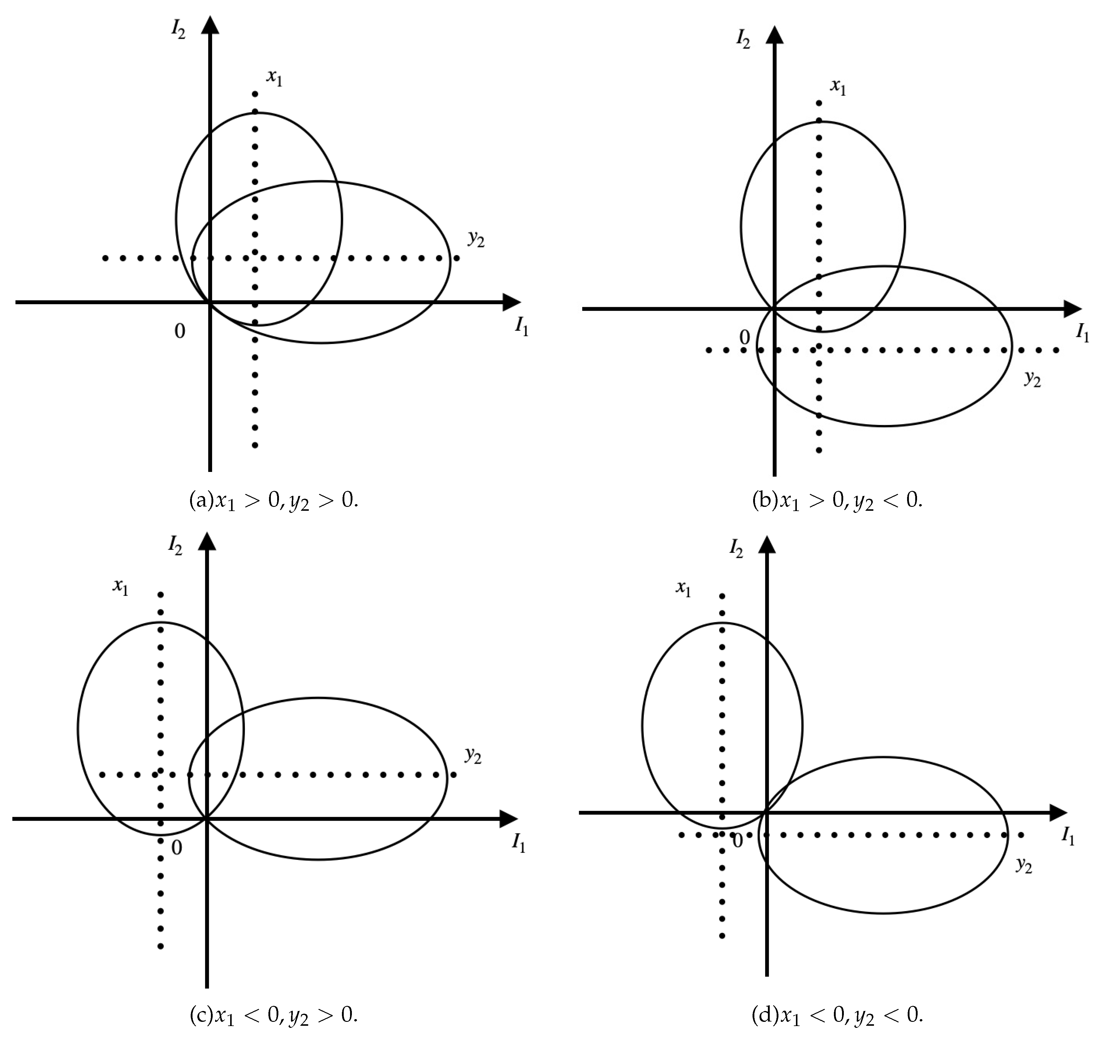
Eq. (3) and (4) can be written as two ellipses,
I 1 x 1 2 a 1 2 + I 2 y 1 2 b 1 2 = 1 , I 1 x 2 2 a 2 2 + I 2 y 2 2 b 2 2 = 1 .
Where,
x 1 = 1 2 N 1 1 b + d + α N 1 γ e μ τ , y 1 = 1 2 N 2 1 + 1 N 2 γ e μ τ , x 2 = 1 2 N 1 1 + 1 N 1 γ e μ τ , y 2 = 1 2 N 2 1 b + d + α N 2 γ e μ τ ,
a 1 2 = β e μ τ x 1 2 + 1 θ e 1 θ d γ α e μ τ y 1 2 β e μ τ , b 1 2 = β e μ τ x 1 2 + 1 θ e 1 θ d γ α e μ τ y 1 2 1 θ e 1 θ d γ α e μ τ , a 2 2 = 1 θ e 1 θ d γ α e μ τ x 2 2 + β e μ τ y 2 2 1 θ e 1 θ d γ α e μ τ , b 2 2 = 1 θ e 1 θ d γ α e μ τ x 2 2 + β e μ τ y 2 2 β e μ τ .
We know these two ellipses must pass through the origin, where x 2 > 0 , y 1 > 0 , while the positive or negative cases of x 1 and y 2 remain uncertain. Therefore, we consider I 1 as the horizontal axis and I 2 as the vertical axis to determine the intersection point of the two ellipses in the Cartesian coordinate system, as shown in Figure 2. From Figure 2, we observe that in the first quadrant, the two ellipses have one and only one intersection point. Thus, system (1) exists a unique positive equilibrium P * when R 0 > 1 . Of course, we cannot express the specific expression of P * . There are also special positive equilibriums, such as the one proposed by Liu [33].
Theorem 2. 
If R 0 < 1 , the disease-free equilibrium P 0 of model (1) is locally asymptotically stable.
Proof 
The Jacobian matrix of model (1) at P 0 is:
J = A O B O C M D N B O A O D N C M ,
Where, O is the zero matrix,
A = α μ β S 0 0 β S 0 e λ τ e μ τ b + d + α ,
B = α 1 θ d γ α S 0 0 1 θ e 1 θ d γ α S 0 e λ τ e μ τ + 1 θ e 1 θ d α ,
C = 0 θ d α 0 d , D = 0 θ e ( 1 θ d ) γ α S 0 + θ e ( 1 θ d ) α 0 0 ,
M = ( c + f ) 0 f ( α + μ ) , N = 0 0 0 α .
The equation of characteristics of model (1) at the disease-free equilibrium P 0 is
J 1 = ( λ + α + μ ) 2 ( λ + c + f ) 2 ( λ + μ ) ( λ + 2 α + μ ) [ λ + d + b + α 1 θ e 1 θ d α β + 1 θ e 1 θ d γ α S 0 e μ τ e λ τ ] [ λ + d + b + α + 1 θ e 1 θ d α β 1 θ e 1 θ d γ α S 0 e μ τ e λ τ ] = 0 .
The characteristic polynomial has negative roots λ 1 = μ , λ 2 = 2 α + μ , λ 3 = ( α + μ ) , λ 4 = ( c + f ) , and the remaining roots are obtained from the following:
λ + d + b + α 1 θ e 1 θ d α = β + 1 θ e 1 θ d γ α S 0 e μ τ e λ τ ,
λ + d + b + α + 1 θ e 1 θ d α = β 1 θ e 1 θ d γ α S 0 e μ τ e λ τ .
We assume that λ has a nonnegative real part, modulo both sides of the above two equations (6) and (7), and the left side of the equations is
λ + d + b + α 1 θ e 1 θ d α > d + b + θ d α + θ e 1 θ d α , λ + d + b + α + 1 θ e 1 θ d α > d + b + α + 1 θ e 1 θ d α > d + b + θ d α + θ e 1 θ d α .
The right side of the equations is
β + 1 θ e 1 θ d γ α S 0 e μ τ e λ τ < β + 1 θ e 1 θ d γ α S 0 e μ τ , β 1 θ e 1 θ d γ α S 0 e μ τ e λ τ < β + 1 θ e 1 θ d γ α S 0 e μ τ .
When R 0 < 1 ,
β + 1 θ e 1 θ d γ α S 0 e μ τ e λ τ < b + d + θ d α + θ e 1 θ d α .
When R 0 < 1 , λ = 0 is not the root of model (1), so λ does not have the nonnegative real part. This contradicts the assumption that λ has negative real part, i.e., the disease-free equilibrium P 0 of model (1) is locally asymptotically stable. □
Theorem 3. 
If R 0 < 1 , the disease-free equilibrium P 0 of model (1) is globally asymptotically stable.
Proof 
Let us take the following Lyapunov functional into account
V ( t ) = I 1 + I 2 + t τ t β S 1 ( ϕ ) I 1 ( ϕ ) e μ τ + 1 θ e 1 θ d γ α S 2 ( ϕ ) I 2 ( ϕ ) e μ τ d ϕ + t τ t β S 2 ( ϕ ) I 2 ( ϕ ) e μ τ + 1 θ e 1 θ d γ α S 1 ( ϕ ) I 1 ( ϕ ) e μ τ d ϕ .
The time derivative of it along the solutions of model (1) is
V ( t ) ˙ = β + 1 θ e 1 θ d γ α e μ τ S 1 I 1 + S 2 I 2 b + d + θ d α + θ e 1 θ d α I 1 + I 2 β + 1 θ e 1 θ d γ α Λ μ e μ τ I 1 + I 2 b + d + θ d α + θ e 1 θ d α I 1 + I 2 = b + d + θ d α + θ e 1 θ d α R 0 1 I 1 + I 2 .
When R 0 < 1 ,
b + d + θ d α + θ e 1 θ d α R 0 1 I 1 + I 2 < 0 .
In delay differential systems, by LaSalle’s invariance principle, the disease-free equilibrium P 0 of model (1) is globally asymptotically stable. □
Figure 2. The four possible cases of two ellipses given by (5) when R 0 > 1 .
Preprints 108269 g002

3. Data Fitting and Sensitivity Analysis of R 0

3.1. Data Fitting

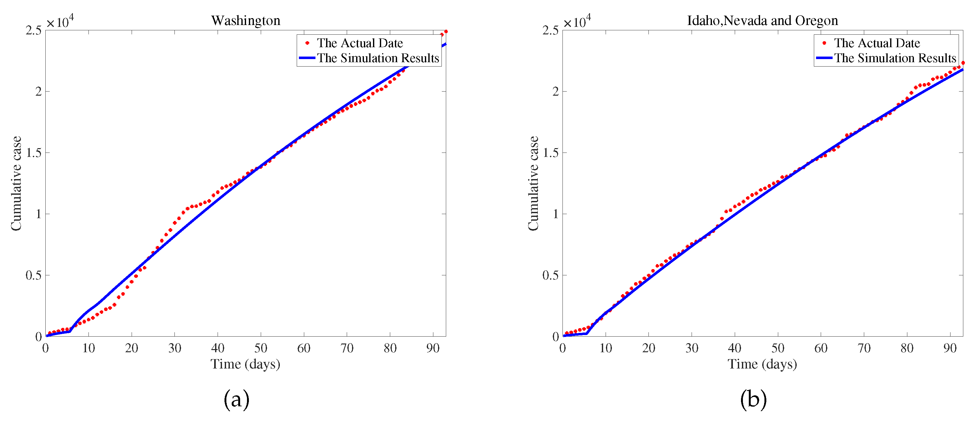
In order to better evaluate the effectiveness of transportation-related infection and exit-entry screenings in preventing and controlling emerging infectious diseases, we will choose actual case data to illustrate. We take the COVID-19 epidemic in the United States as an example. On January 20, 2020, the first confirmed case of COVID-19 was reported in the US, Washington [36], so we take Washington as the hypothetical region 1 and select the surrounding three states of Idaho, Nevada, and Oregon as the hypothetical region 2.
In 2020, the average life expectancy of the U.S. population was 77.0 years [37], approximately 300 new births occur in Washington every day [38]. Therefore, we choose the range of Λ to be ( 0 , 300 ) , and the natural death rate μ is 1 / 365 × 77.0 = 3.56 × 10 5 . We choose data ranging from June 10, 2020, to September 10, 2020. In Washington, the number of daily deaths due to illness per 100 , 000 people ranges from approximately 100 to 300 [39]. Therefore, the range for the average death rate of the infected b is ( 0.001 , 0.003 ) . The estimated hospitalization death rate of isolated infected individuals ranges from 5% and 20% [40], so we choose the range for the average death rate of isolated infected individuals c to be ( 0.05 , 0.2 ) . Lightly symptomatic patients typically recover in 7 to 14 days, while severely symptomatic patients may take 1 to 2 months to recover [41]. We choose the same range for the recovery rate per capita during isolation treatment f and the per capita rate of natural recovery d, which is ( 0.016 , 0.14 ) . The incubative period of COVID-19 is typically between 2 and 14 days, so the range for the incubative period τ is ( 2 , 14 ) [42]. According to the actual prevention and control situation in the United States at that time [43,44], we make some assumptions on the parameters of the model (1). We assume that 10% of the people in Washington, Idaho, Nevada, and Oregon flow daily, and the upper limit of the migration rate is 0.1 × 1 = 0.1 . Considering that all people leave Washington to go to Idaho, Nevada, and Oregon, or leave Idaho, Nevada, and Oregon to travel to Washington at least once a year with a lower limit of mobility is 1 / 365 = 0.0027 , the range of α is ( 0.0027 , 0.1 ) . Assuming that the success rate of entry and exit screening is less than half, the θ e and θ d ranges are ( 0.1 , 0.5 ) . We obtain the parameter range of Table 2.
Since the data we use is cumulative confirmed cases from the Population Health Institute of the Robert Wood Johnson Foundation at the University of Wisconsin [45], before conducting data fitting, we need to add two cumulative confirmed cases compartments represented by C i ( i = 1 , 2 ) :
d C 1 d t = β S 1 ( t τ ) I 1 ( t τ ) e μ τ + 1 θ e 1 θ d γ α S 2 ( t τ ) I 2 ( t τ ) e μ τ + 1 θ e 1 θ d α I 2 , d C 2 d t = β S 2 ( t τ ) I 2 ( t τ ) e μ τ + 1 θ e 1 θ d γ α S 1 ( t τ ) I 1 ( t τ ) e μ τ + 1 θ e 1 θ d α I 1 .
The initial values S 1 ( 0 ) = 7 × 10 6 , S 2 ( 0 ) = 9 × 10 6 , I 1 ( 0 ) = 300 , I 2 ( 0 ) = 200 , Q 1 ( 0 ) = 0 , Q 2 ( 0 ) = 0 , R 1 ( 0 ) = 0 , R 2 ( 0 ) = 0 are selected. We use the method proposed by Zhang [46] and Li et al. [47,48] to carry out parameter estimation and data fitting, and the estimated optimal parameter values can be seen in Table 2.
Figure 3 displays the accumulated confirmed cases in Washington, Idaho, Nevada, and Oregon under the actual data. The simulation results are consistent with the actual data, proving that model (1) is more suitable to simulate the outbreak and epidemic of emerging infectious diseases.

3.2. Sensitivity Analysis of R 0

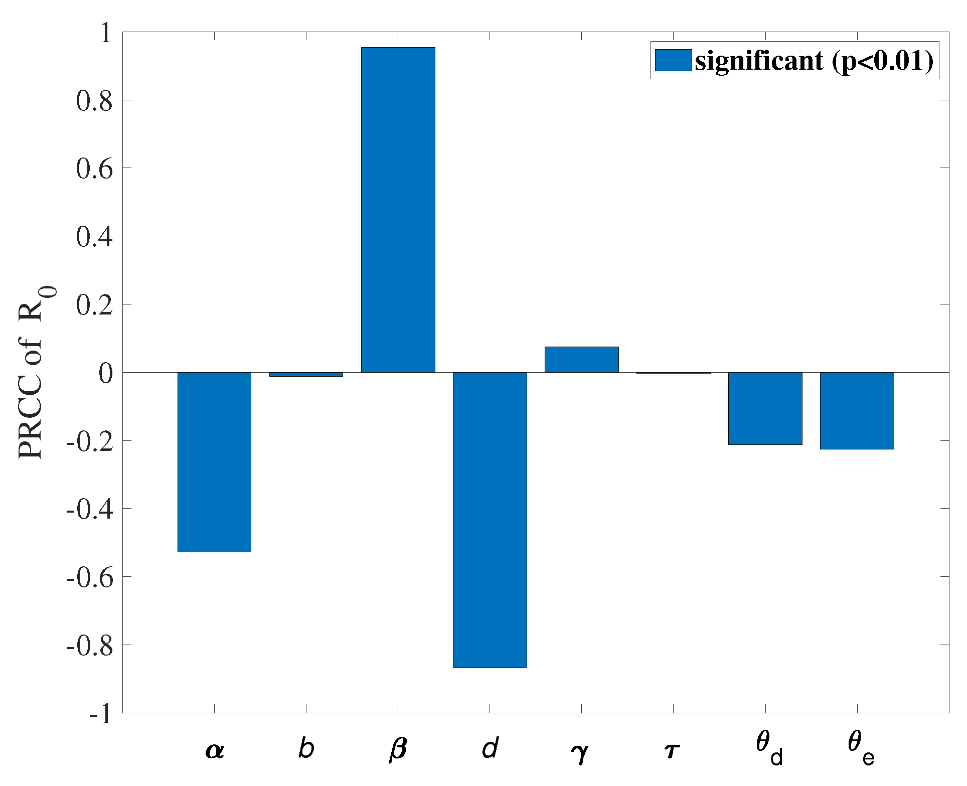
Sensitivity analysis is performed to discern the degree of correlation between the input parameters and the predicted ones, as well as to figure out the necessary degree of variation in the input parameters to achieve the expected value of the parameters. Generally speaking, the beginning of disease transmission is directly affected by the basic reproduction number R 0 . In this segment, in order to study the effectiveness of COVID-19 control strategies in the United States, we calculate the sensitivity index of R 0 , whose purpose is to survey the relative alterations in R 0 as the model parameters changes. Then, we ponder the parameters from Table 2. Sensitivity analysis based on PRCC evaluated the effect of parameters on the response function, i.e., basic reproduction number R 0 . We take the sample size N = 10000 , in addition to λ , μ , all parameters as the input variables, the value of R 0 as output variables. It can be obtained from Figure 4 which shows that β the most sensitive parameter then followed d, α , θ d , θ e , γ , τ .
We propose adequate measures for preventing and controlling COVID-19 based on sensitivity analysis. These measures include wearing masks to interrupt transmission pathways, implementing city lockdowns to control population movement, and timely medication for patients who are ill but have not yet been hospitalized. Implementing these measures can enhance the effectiveness of prevention and control efforts. In the next part, we are going to explore the best control ways.

4. Optimal Control Strategies

Owing to the previous R 0 sensitivity analysis and combined with the reality of COVID-19 in America, we put our hands to seek an effective way to control COVID-19 infections. u 1 ( t ) aims to control the transmission rate of susceptible people, which is measured by preventive measures like wearing masks and reducing gatherings. u 2 ( t ) aims to control population migration, measured through policy interventions and city lockdowns. u 3 ( t ) aims to take medication and actively pursue treatment to enhance the natural recovery rate. With all the assumptions we mentioned above, the time-delayed model takes the control problem as follows:
d S 1 d t = Λ β 1 u 1 S 1 I 1 α 1 u 2 S 1 + α 1 u 2 S 2 1 θ d γ α 1 u 2 S 2 I 2 μ S 1 , d I 1 d t = β 1 u 1 S 1 ( t τ ) I 1 ( t τ ) e μ τ + 1 θ d 1 θ e γ α 1 u 2 S 2 ( t τ ) I 2 ( t τ ) e μ τ + 1 θ d 1 θ e α 1 u 2 I 2 b + d 1 + u 3 + α 1 u 2 I 1 , d Q 1 d t = θ e 1 θ d γ α 1 u 2 S 2 I 2 + θ d α 1 u 2 I 1 + θ e 1 θ d α 1 u 2 I 2 ( c + f ) Q 1 , d R 1 d t = f Q 1 + d 1 + u 3 I 1 α 1 u 2 R 1 + α 1 u 2 R 2 μ R 1 , d S 2 d t = Λ β 1 u 1 S 2 I 2 α 1 u 2 S 2 + α 1 u 2 S 1 1 θ d γ α 1 u 2 S 1 I 1 μ S 2 , d I 2 d t = β 1 u 1 S 2 ( t τ ) I 2 ( t τ ) e μ τ + 1 θ d 1 θ e γ α 1 u 2 S 1 ( t τ ) I 1 ( t τ ) e μ τ + 1 θ d 1 θ e α 1 u 2 I 1 b + d 1 + u 3 + α 1 u 2 I 2 , d Q 2 d t = θ e 1 θ d γ α 1 u 2 S 1 I 1 + θ d α 1 u 2 I 2 + θ e 1 θ d α 1 u 2 I 1 ( c + f ) Q 2 , d R 2 d t = f Q 2 + d 1 + u 3 I 2 α 1 u 2 R 2 + α 1 u 2 R 1 μ R 2 .
The initial conditions
S 1 ( δ ) = ϕ 1 ( δ ) , I 1 ( δ ) = ϕ 2 ( δ ) , Q 1 ( δ ) = ϕ 3 ( δ ) , R 1 ( δ ) = ϕ 4 ( δ ) , S 2 ( δ ) = ϕ 5 ( δ ) , I 2 ( δ ) = ϕ 6 ( δ ) , Q 2 ( δ ) = ϕ 7 ( δ ) , R 2 ( δ ) = ϕ 8 ( δ ) , ϕ i ( δ ) 0 , δ [ τ , 0 ] , ϕ i ( 0 ) > 0 , ϕ i ( δ ) C [ τ , 0 ] , R + , i = 1 , 2 , , 8 .
Regarding variables u i ( t ) ( i = 1 , 2 , 3 ) and the above control system, considering that the spread of emerging infectious diseases is related to transportation-related infections between two regions, we consider reducing the number of patients who are not successfully detected in entry and exit screenings between the two regions.
Our objective function J ( u 1 ( t ) , u 2 ( t ) , u 3 ( t ) ) is defined as
J ( u 1 ( t ) , u 2 ( t ) , u 3 ( t ) ) = 0 T [ A 1 ( 1 θ d ) ( 1 θ e ) α I 1 + A 2 ( 1 θ d ) ( 1 θ e ) α I 2 + 1 2 ( B 1 u 1 2 ( t ) + B 2 u 2 2 ( t ) + B 3 u 3 2 ( t ) ) ] d t ,
where the interval [ 0 , T ] signifies the time duration of the control program, the quantities A i ( i = 1 , 2 ) represents the weight constants of patients in region 1 and region 2 who were not successfully detected. B i ( i = 1 , 2 , 3 ) represents the transmission rate of the susceptible population. In every region i, the susceptible and infected individuals move to region j at a per capita rate α ( i , j = 1 , 2 , i j ) and the per capita rate of natural recovery from disease. Constants A i , ( i = 1 , 2 ) , B i , ( i = 1 , 2 , 3 ) signify a measure of the relative cost of the interventions over the interval [ 0 , T ] . The expression ( 1 θ d ) ( 1 θ e ) α I i , ( i = 1 , 2 ) refers to the patients who are not successfully detected between two regions. Therefore, this term is included in the objective function. In addition, we should consider the costs of wearing masks, city lockdowns, and purchasing medications. Our goal is to find the optimal control ( u 1 , u 2 , u 3 ) such as
J u 1 * ( t ) , u 2 * ( t ) , u 3 * ( t ) = min J u 1 ( t ) , u 2 ( t ) , u 3 ( t ) u 1 ( t ) , u 2 ( t ) , u 3 ( t ) U ,
the control set U equals that
U = u 1 ( t ) , u 2 ( t ) , u 3 ( t ) u i ( t ) ( i = 1 , 2 , 3 ) can be measured , u i ( t ) ( 0 , 1 ) , t [ 0 , T ] .
Through the Filippov–Cesari Existence Theorem and the Mangasarian Theorem [49], a special method u 1 * ( t ) , u 2 * ( t ) , u 3 * ( t ) which is the optimal control exists. After that, we can find this method in Pontryagin’s Minimum Principle [50].
Theorem 4. 
Suppose u 1 * , u 2 * and u 3 * are the optimal control variables, and correspondingly S 1 * , I 1 * , Q 1 * , R 1 * , S 2 * , I 2 * , Q 2 * , R 2 * are the control system’s (8) optimal state variables, then there exists adjoint variable λ ( t ) = ( λ 1 ( t ) , λ 2 ( t ) , λ 3 ( t ) , λ 4 ( t ) , λ 5 ( t ) , λ 6 ( t ) , λ 7 ( t ) , λ 8 ( t ) ) R 8 that satisfies the following adjoint equations:
d λ 1 ( t ) d t = λ 1 ( t ) β 1 u 1 I 1 + μ + λ 5 ( t ) λ 7 ( t ) θ e 1 θ d γ α 1 u 2 I 1 χ [ 0 , T τ ] ( t ) β 1 u 1 I 1 ( t τ ) e μ τ λ 2 ( t + τ ) + λ 1 ( t ) λ 5 ( t ) α 1 u 2 χ [ 0 , T τ ] ( t ) 1 θ d 1 θ e γ α 1 u 2 I 1 ( t τ ) e μ τ λ 6 ( t + τ ) , d λ 2 ( t ) d t = A 1 ( 1 θ d ) ( 1 θ e ) α + λ 1 ( t ) β 1 u 1 S 1 + λ 2 ( t ) b + d 1 + u 3 + α 1 u 2 λ 4 ( t ) ( 1 + d u 3 ) + λ 5 ( t ) 1 θ d γ α ( 1 u 2 S 1 λ 7 ( t ) θ e 1 θ d γ α 1 u 2 S 1 λ 6 ( t ) 1 θ d 1 θ e α 1 u 2 λ 7 ( t ) θ e 1 θ d α ( 1 u 2 ) χ [ 0 , T τ ] ( t ) β 1 u 1 S 1 ( t τ ) e μ τ λ 2 ( t + τ ) λ 3 ( t ) θ d α ( 1 u 2 ) χ [ 0 , T τ ] ( t ) ( 1 θ d ) ( 1 θ e ) γ α ( 1 u 2 S 1 ( t τ ) e μ τ λ 6 ( t + τ ) , d λ 3 ( t ) d t = λ 3 ( t ) ( c + f ) λ 4 ( t ) f , d λ 4 ( t ) d t = λ 4 ( t ) λ 8 ( t ) α 1 u 2 + λ 4 ( t ) μ , d λ 5 ( t ) d t = λ 5 ( t ) β 1 u 1 I 2 + μ + λ 1 ( t ) λ 3 ( t ) θ e 1 θ d γ α 1 u 2 I 2 χ [ 0 , T τ ] ( t ) β 1 u 1 I 2 ( t τ ) e μ τ λ 6 ( t + τ ) + λ 5 ( t ) λ 1 ( t ) α 1 u 2 χ [ 0 , T τ ] ( t ) 1 θ d 1 θ e γ α 1 u 2 I 2 ( t τ ) e μ τ λ 2 ( t + τ ) , d λ 6 ( t ) d t = A 2 ( 1 θ d ) ( 1 θ e ) α + λ 5 ( t ) β 1 u 1 S 2 + λ 6 ( t ) b + d 1 + u 3 + α 1 u 2 λ 8 ( t ) ( 1 + d u 3 ) + λ 1 ( t ) 1 θ d γ α ( 1 u 2 S 2 λ 3 ( t ) θ e 1 θ d γ α 1 u 2 S 2 λ 2 ( t ) 1 θ d 1 θ e α 1 u 2 λ 3 ( t ) θ e 1 θ d α ( 1 u 2 χ [ 0 , T τ ] ( t ) β 1 u 1 S 2 ( t τ ) e μ τ λ 6 ( t + τ ) λ 7 ( t ) θ d α ( 1 u 2 ) χ [ 0 , T τ ] ( t ) 1 θ d 1 θ e γ α ( 1 u 2 S 2 ( t τ ) e μ τ λ 2 ( t + τ ) , d λ 7 ( t ) d t = λ 7 ( t ) ( c + f ) λ 8 ( t ) f , d λ 8 ( t ) d t = λ 8 ( t ) λ 4 ( t ) α 1 u 2 + λ 8 ( t ) μ .
Given the transversality conditions λ i ( T ) = 0 ( i = 1 , 2 , 3 , 4 , 5 , 6 , 7 , 8 ) . Moreover, we provide the corresponding parameters below:
u 1 * ( t ) = min 1 , max 0 , u ¯ 1 ( t ) , u 2 * ( t ) = min 1 , max 0 , u ¯ 2 ( t ) , u 3 * ( t ) = min 1 , max 0 , u ¯ 3 ( t ) .
u ¯ 1 ( t ) = λ 2 ( t ) β S 1 ( t τ ) I 1 ( t τ ) e μ τ + λ 6 ( t ) β S 2 ( t τ ) I 2 ( t τ ) e μ τ λ 5 ( t ) β S 2 I 2 λ 1 ( t ) β S 1 I 1 B 1 , u ¯ 2 ( t ) = λ 2 ( t ) 1 θ d 1 θ e γ α S 2 ( t τ ) I 2 ( t τ ) e μ τ + 1 θ d 1 θ e α I 2 α I 1 + λ 3 ( t ) θ e 1 θ d γ α S 2 I 2 + θ d α I 1 + θ e 1 θ d α I 2 + λ 6 ( t ) 1 θ d 1 θ e γ α S 1 ( t τ ) I 1 ( t τ ) e μ τ + 1 θ d 1 θ e α I 1 α I 2 + λ 7 ( t ) θ e 1 θ d γ α S 1 I 1 + θ d α I 2 + θ e 1 θ d α I 1 λ 8 ( t ) λ 4 ( t ) α R 1 α R 2 λ 1 ( t ) α S 1 α S 2 + 1 θ d γ α S 2 I 2 λ 5 ( t ) α S 2 α S 1 + 1 θ d γ α S 1 I 1 / B 2 , u ¯ 3 ( t ) = λ 2 ( t ) λ 4 ( t ) d I 1 + λ 6 ( t ) λ 8 ( t ) d I 2 B 3 .
Proof. 
The control problem of the Hamilton function H is defined as
H ( t ) = A 1 ( 1 θ d ) ( 1 θ e ) α I 1 + A 2 ( 1 θ d ) ( 1 θ e ) α I 2 + 1 2 B 1 u 1 2 ( t ) + B 2 u 2 2 ( t ) + B 3 u 3 2 ( t ) + λ 1 ( t ) Λ β 1 u 1 S 1 I 1 α 1 u 2 S 1 + α 1 u 2 S 2 1 θ d γ α 1 u 2 S 2 I 2 μ S 1 + λ 2 ( t ) β 1 u 1 S 1 ( t τ ) I 1 ( t τ ) e μ τ + 1 θ d 1 θ e γ α 1 u 2 S 2 ( t τ ) I 2 ( t τ ) e μ τ + 1 θ d 1 θ e α 1 u 2 I 2 b + d 1 + u 3 + α 1 u 2 I 1 + λ 3 ( t ) θ e 1 θ d γ α 1 u 2 S 2 I 2 + θ d α 1 u 2 I 1 + θ e 1 θ d α 1 u 2 I 2 ( c + f ) Q 1 + λ 4 f Q 1 + d 1 + u 3 I 1 α 1 u 2 R 1 + α 1 u 2 R 2 μ R 1 + λ 5 ( t ) Λ β 1 u 1 S 2 I 2 α 1 u 2 S 2 + α 1 u 2 S 1 1 θ d γ α 1 u 2 S 1 I 1 μ S 2 + λ 6 ( t ) β 1 u 1 S 2 ( t τ ) I 2 ( t τ ) e μ τ + 1 θ d 1 θ e γ α 1 u 2 S 1 ( t τ ) I 1 ( t τ ) e μ τ + 1 θ d 1 θ e α 1 u 2 I 1 b + d 1 + u 3 + α 1 u 2 I 2 + λ 7 ( t ) θ e 1 θ d γ α 1 u 2 S 1 I 1 + θ d α 1 u 2 I 2 + θ e 1 θ d α 1 u 2 I 1 ( c + f ) Q 2 + λ 8 f Q 2 + d 1 + u 3 I 2 α 1 u 2 R 2 + α 1 u 2 R 1 μ R 2 ,
where λ ( t ) = ( λ 1 ( t ) , λ 2 ( t ) , λ 3 ( t ) , λ 4 ( t ) , λ 5 ( t ) , λ 6 ( t ) , λ 7 ( t ) , λ 8 ( t ) ) T is the adjoint variable satisfying
d λ 1 ( t ) d t = H S 1 ( t ) χ [ 0 , T τ ] ( t ) H S 1 ( t τ ) ( t + τ ) ,
d λ 2 ( t ) d t = H I 1 ( t ) χ [ 0 , T τ ] ( t ) H I 1 ( t τ ) ( t + τ ) ,
d λ 3 ( t ) d t = H Q 1 ( t ) ,
d λ 4 ( t ) d t = H R 1 ( t ) ,
d λ 5 ( t ) d t = H S 2 ( t ) χ [ 0 , T τ ] ( t ) H S 2 ( t τ ) ( t + τ ) ,
d λ 6 ( t ) d t = H I 2 ( t ) χ [ 0 , T τ ] ( t ) H I 2 ( t τ ) ( t + τ ) ,
d λ 7 ( t ) d t = H Q 2 ( t ) ,
d λ 8 ( t ) d t = H R 2 ( t ) .
On [ 0 , T τ ] , χ [ T τ ] ( t ) are indicator functions under the transversality conditions λ i ( T ) = 0 ( i = 1 , 2 , 3 , 4 , 5 , 6 , 7 , 8 ) , which fullfill
χ [ T τ ] ( t ) = 1 , t [ 0 , T τ ] , 0 , o t h e r w i s e .
The optimality equation
H u 1 ( t ) = H u 2 ( t ) = H u 3 ( t ) = 0 .
From the optimality equation,
B 1 u 1 + λ 1 ( t ) β S 1 I 1 λ 2 ( t ) β S 1 ( t τ ) I 1 ( t τ ) e μ τ + λ 5 ( t ) β S 2 I 2 λ 6 ( t ) β S 2 ( t τ ) I 2 ( t τ ) e μ τ = 0 , B 2 u 2 + λ 1 ( t ) α S 1 α S 2 + 1 θ d γ α S 2 I 2 λ 2 ( t ) 1 θ d 1 θ e γ α S 2 ( t τ ) I 2 ( t τ ) e μ τ + 1 θ d 1 θ e α I 2 α I 1 λ 3 ( t ) θ e 1 θ d γ α S 2 I 2 + θ d α I 1 + θ e 1 θ d α I 2 + λ 5 ( t ) α S 2 α S 1 + 1 θ d γ α S 1 I 1 λ 6 ( t ) 1 θ d 1 θ e γ α S 1 ( t τ ) I 1 ( t τ ) e μ τ + 1 θ d 1 θ e α I 1 α I 2 λ 7 ( t ) θ e 1 θ d γ α S 1 I 1 + θ d α I 2 + θ e 1 θ d α I 1 λ 8 ( t ) λ 4 ( t ) α R 1 α R 2 = 0 , B 3 u 3 λ 2 ( t ) λ 4 ( t ) d I 1 λ 6 ( t ) λ 8 ( t ) d I 2 = 0 .
Thus we have,
u ¯ ( t ) = u ¯ 1 ( t ) , u ¯ 2 ( t ) , u ¯ 3 ( t ) .
Given that u * ( t ) is part of U, we see
u 1 * ( t ) = min 1 , max 0 , u ¯ 1 ( t ) , u 2 * ( t ) = min 1 , max 0 , u ¯ 2 ( t ) , u 3 * ( t ) = min 1 , max 0 , u ¯ 3 ( t ) .
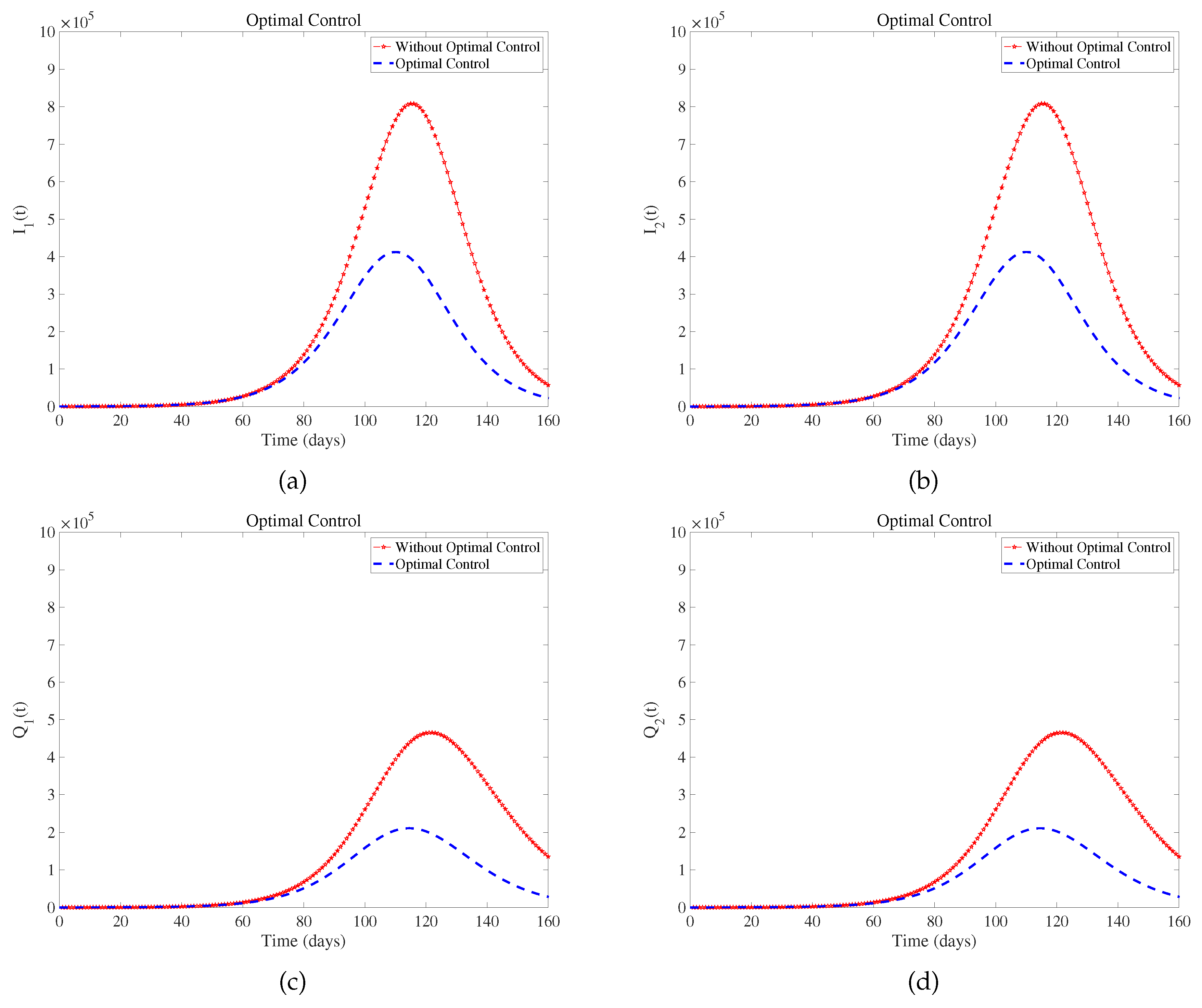
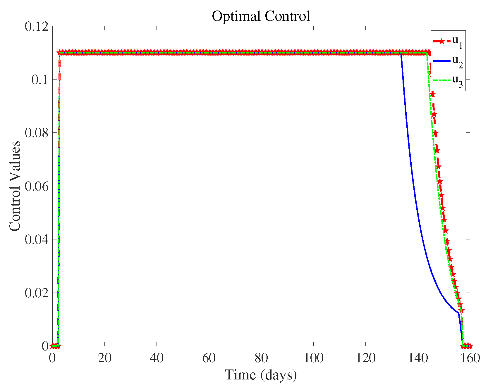
We present some numerical outcomes that belong to the optimality system. In order to determine the optimal control and the state system, we use the scheme proposed in [47,50], which is based on the forward-backward sweep scheme. Furthermore, many other algorithms describe approximation methods for obtaining optimal control [51,52]. We choose the figure from Table 2 as the parameter values in the optimal control. The weights in the goal function A 1 = A 2 = 10 , B 1 = 20 , B 2 = 80 , B 3 = 120 , we will explain these values in next section. The results in Figure 5 suggest that optimal control effectively controls the development and deterioration of the disease. In fact, the intensity of various measures implemented by the government is different, such as wearing masks. Combined with the prevention and control situation in the United States at that time[53,54,55], we assume that the upper limit of these three measures is 0.11 . Figure 6 shows the control intensity of each measure in the control system over time, and we can see the magnitude of these three measures when they are taken at the same time. u 2 ( t ) (controlling population migration) can end about 20 days earlier than u 1 ( t ) (wearing masks) and u 3 ( t ) (take medication and actively pursue treatment). This means that we can reduce the control intensity of u 2 ( t ) (controlling population migration) sometime in advance when all three measures are implemented. Implementing various strategies has a certain cost, and we discuss the most cost-effective strategies in the next section.

5. Cost-Effectiveness Analysis

We use three ways, which are: infection averted ratio (IAR) [56], average cost-effectiveness ratio (ACER) [57], and incremental cost-effectiveness ratio (ICER) [57] to complete the cost-effectiveness analysis. Below are the interpretations of the three ways:
(1) IAR can be denoted as
IAR = Number of people avoiding infection Number of people who have recovered after infected .
We regard the control way whose IAR is the highest as the economical choice [57].
(2) ACER is told as
ACER = The overall cos t resulting from the carrying out of a specific intervention strategy Numeber of people who have avioding infection after performing strategy .
We assess the money which is used to perform a particular intervention strategy is
c ( u ) = 1 2 0 T i = 1 3 B i u i 2 d t .
(3) ICER assess the variations in cost and health advantages of two distinct intervention strategies under the same limited resourses. Viewing strategies m and n as two viral control intervention strategies, then ICER is expressed as
ICER = Total cos t variations in strategies m and n Control benefits variations in strategies m and n .
The infection that is prevented with the controls during the time period T is expressed as
I n f e c t i o n a v e r t e d = T I 1 ( 0 ) + I 2 ( 0 ) 0 T I 1   * ( t ) + I 2   * ( t ) d t .
Here, B i , ( i = 1 , 2 , 3 ) is related to the per capita unit cost of the measures u i * , i = 1 , 2 , 3 . Let us take the example of Washington. Washington mandates wearing masks in public settings [53]. However, due to cost and availability, individuals in low-income environments are likelier to use reusable cloth masks instead of disposable medical masks. There is still uncertainty in mask-wearing practices, such as the duration of wearing a mask [58]. Therefore, we can reasonably assume that the daily cost of a mask for each person is approximately 0.06 dollars, which amounts to approximately 21.9 dollars per year.
Due to early stay-at-home orders in the United States, population mobility and migration decreased [54], and local governments also provided subsidies to the public during the pandemic [55]. We assume the average annual subsidy per person is approximately 80 dollars. As the prices of different drugs for treating and preventing COVID-19 vary [59,60], we assume that the annual cost for each person to purchase drugs for COVID-19 treatment is approximately 120 dollars.
Because of the specific numerical values given by the fourth column of Table 3, it is clear that Strategy 1 (wearing a mask) is the most cost-effective measure.
According to the ACER values in column 5 of Table 3, Strategy 1 is the lowest, so the most cost-effective Strategy is Strategy 1 (wearing masks).
Next, we calculate the ICER value, where we rank the number of people we want to avoid infection in increasing order.
The ICER is computed as
ICER ( 3 ) = 2.188 × 10 7 0 1.823 × 10 5 0 = 120.021 , ICER ( 2 ) = 4.921 × 10 7 2.188 × 10 7 6.152 × 10 5 1.823 × 10 5 = 63.132 , ICER ( 6 ) = 7.109 × 10 7 4.921 × 10 7 6.157 × 10 5 6.152 × 10 5 = 599.452 , ICER ( 1 ) = 1.515 × 10 7 7.109 × 10 7 6.921 × 10 5 6.517 × 10 5 = 1385.650 , ICER ( 5 ) = 3.703 × 10 7 1.515 × 10 7 7.080 × 10 5 6.921 × 10 5 = 1376.100 , ICER ( 4 ) = 6.436 × 10 7 3.703 × 10 7 8.301 × 10 5 7.080 × 10 5 = 223.833 , ICER ( 7 ) = 8.624 × 10 7 6.436 × 10 7 8.787 × 10 5 8.301 × 10 5 = 450.210 .
The results are presented in Table 3. Compared with the ICER value of Strategy 6, Strategy 5 is significantly superior. Therefore, Strategy 5 is removed from the control list. Similarly, in sequence, we can eliminate strategies 6, 7, 4, 3, and 2. Detailed calculation process can be found in .
Therefore, to sum up the analysis, we can know that when one considers the following control measures: u 1 (wearing masks ), u 2 (policy interventions and city lockdowns), u 3 (taking medication and actively seeking treatment). u 1 (wearing masks) is the least incremental cost-effective, providing the optimal cost over all other strategies on a large scale.

6. Discussion

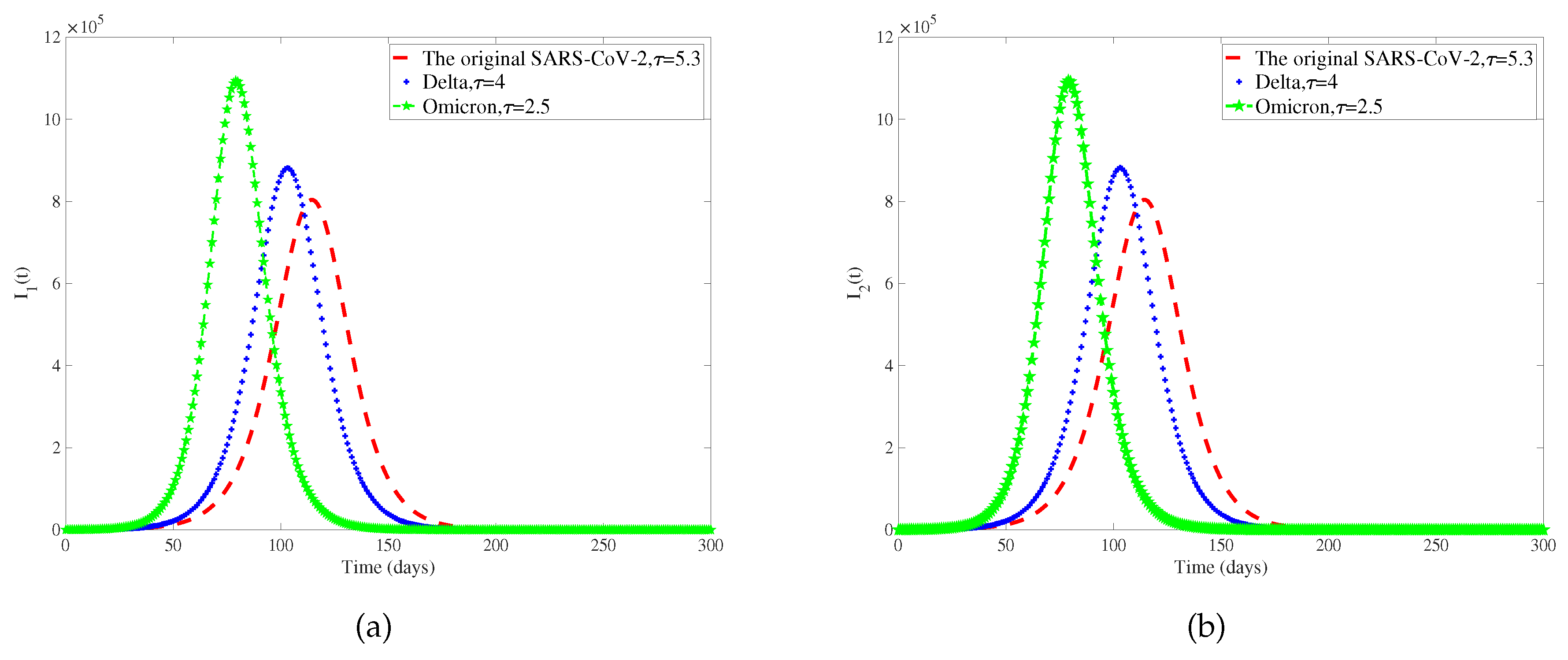
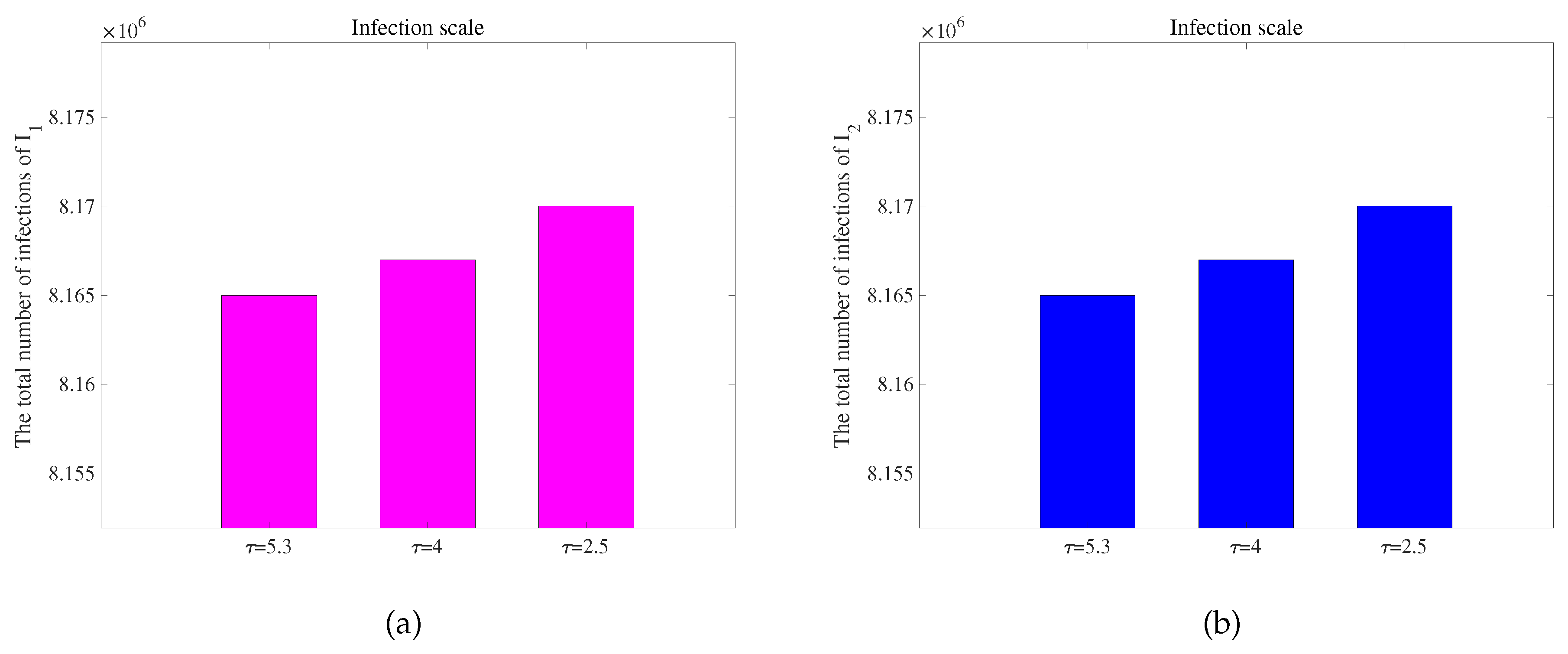
Considering that different genotypes of viruses have different incubative periods, we select different viruses circulating in different periods of COVID-19. The original SARS-CoV-2, Delta, and Omicron incubation periods are 5.3 days, 4 days, and 2.5 days [42,61]. We only discuss the influence of the length of the incubative period on the number of patients, so other parameters in the model are determined, and Figure 7 is obtained. To observe the extent of infection for different incubative periods, we have extracted data on the total quantity of infected individuals in 300 days with different incubative periods in two regions from Figure 7, as shown in Figure 8. We obtain conclusions similar to those of [62]. As the disease incubative period becomes shorter, the disease tends to end earlier, leading to a larger scale of infection.
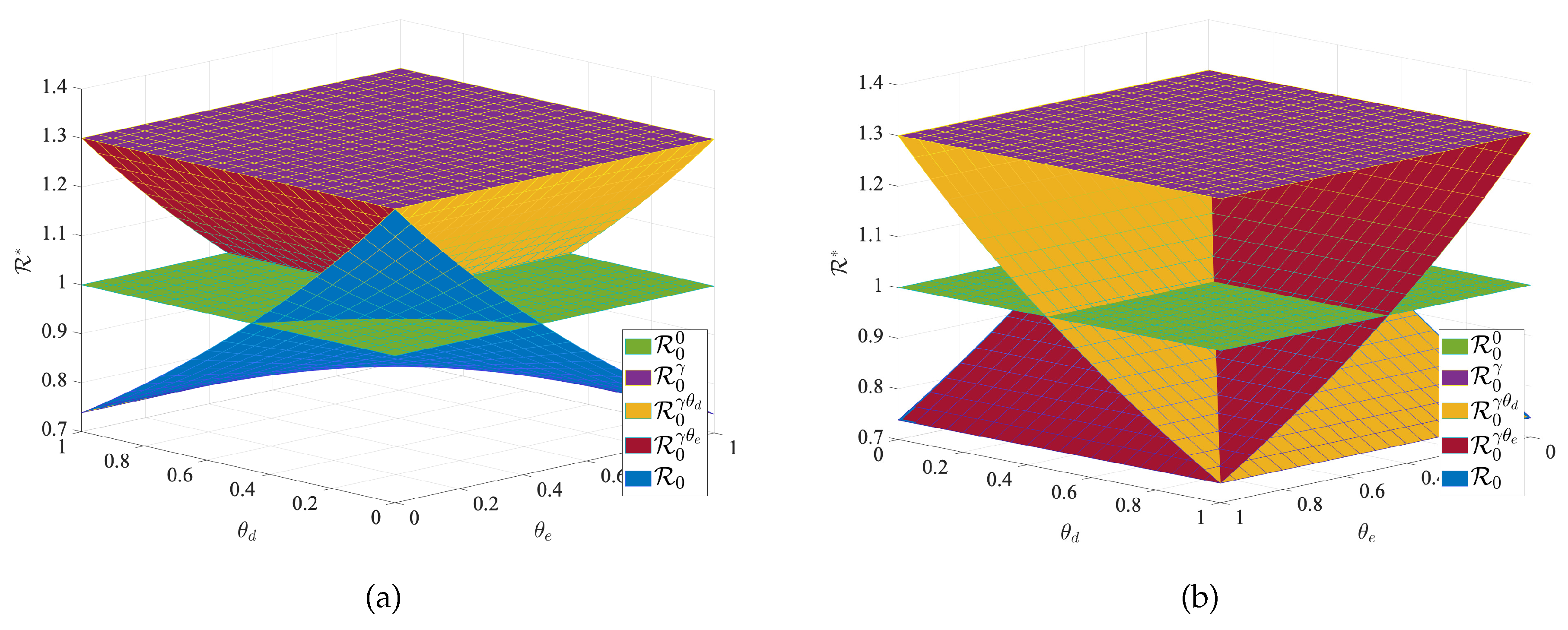
To verify the effectiveness of transportation-related infection and entry-exit screenings, we take the below four reproduction numbers into consideration,
R 0 0 = β S 0 e μ τ b + d , R 0 γ = ( β + γ α ) S 0 e μ τ b + d , R 0 γ θ d = ( β + ( 1 θ d ) γ α ) S 0 e μ τ b + d + θ d α ,
R 0 γ θ e = ( β + ( 1 θ e ) γ α ) S 0 e μ τ b + d + θ e α , R 0 = ( β + 1 θ e 1 θ d γ α ) S 0 e μ τ b + d + θ d α + θ e 1 θ d α .
The R 0 0 is the basic reproduction number for each region when no individuals are moving between regions, and R 0 γ is the basic reproduction number when there is transportation-related infection. R 0 γ θ e is the value of the basic reproduction number for transportation-related infection and entry screening, while R 0 γ θ d is the one for transportation-related infection and exit screening, the R 0 is the basic reproduction number for model (1) with transportation-related infection and entry-exit screenings. In order to consider the effects of θ d and θ e on the disease, we take the basic reproduction number R 0 0 with no population movement between the two cities as the base. We fix all the parameters except θ d and θ e and observe the change in the basic reproduction number. We obtain Figure 9 of R * with respect to θ d and θ e . The results in Figure 9 indicate that transportation-related infections increase the basic reproduction number and enhance disease transmission. Entry or exit screening can inhibit disease transmission by reducing the basic reproduction number.

7. Conclusion

We have established a time-delayed SIQR epidemiological model for infectious diseases with transportation-related infections between two regions. Although many diseases, such as SARS and influenza, can be studied using this model, we focus on using COVID-19 as a specific example to consider our model. Despite the end of the COVID-19 pandemic, it is still essential to remain vigilant and understand how to prevent such emerging diseases in real-time.
We obtain some useful conclusions. Model (1) has a unique global asymptotically stable disease-free equilibrium when R 0 < 1 and a unique endemic equilibrium exists when R 0 > 1 . We use COVID-19 data from Washington, USA, between June 10, 2020, and September 10, 2020, to fit the model and obtain a set of optimal parameters. We conduct a sensitivity analysis on the basic reproduction number ( R 0 ) and obtain that β , α , and d are more sensitive parameters compared to other parameters. Based on these sensitive parameters, we propose three control measures: (1) Wearing masks; (2) Policy interventions and city lockdowns; (3) Taking medication and actively pursuing treatment. Considering infections between regions through travel, we formulate an optimal control problem and find an optimal solution to reduce the number of undetected patients traveling between the two regions. We use Pontryagin’s minimum principle to obtain the optimal solution to achieve our goal. Subsequently, we obtain some numerical results using an optimal control approach based on the forward-backward sweep scheme. The results indicate that the control strategies help reduce infections. We can reduce the control intensity of u 2 ( t ) (controlling population migration) sometime in advance when all three measures ( u 1 ( t ) , u 2 ( t ) , u 3 ( t ) ) are implemented. Additionally, due to a decrease in the number of infected individuals, there is a relative reduction in isolating patients in hospitals, which aids in reducing the required medical resources for significant emergent diseases. We compare the three control strategies using three methods: Infection avoidance ratio (IAR), Average cost-effectiveness ratio (ACER), and Incremental cost-effectiveness Ratio (ICER). Strategy 1 (wearing masks) is the most cost-effective measure. Therefore, in the face of some major emerging infectious diseases, such as SARS, COVID-19, and other diseases. We can all encourage and require people to wear masks.
Finally, we discuss the effects of varying the disease’s incubative period and entry-exit screening on the disease. We observe that a shorter incubative period result in a shorter disease duration but leads to a larger scale of infection, and the peaks are reduced. This has a certain guiding role in the face of many major emerging infectious diseases between two regions. We can formulate some effective prevention and control measures according to the length of the disease’s incubative period, which can reduce the large-scale spread of the disease to a certain extent. Transportation-related infections increase the basic reproduction number ( R 0 ) and enhance disease spread. Entry-exit screening have the ability to curb disease spread by lowering the basic reproduction number. Indeed, our model also has many factors that have not been considered. For instance, when the total populations of the two regions in the model are different, and the migration rates between these regions also vary, what is the impact on the spread of this disease? There are many uncertain factors in disease transmission, so what influence do they have on the disease? The risk of reinfection in recovered patients, differences in disease detection coverage in different regions, and transmission in n regions are all questions that deserve to be explored in the future.
Author Contributions

Conceptualization and methodology, Y. X. and Y. L.; writing—original draft, Y. X.; software and validation, Y. X., Y. W and L. P; writing—review and editing, Y. L., S. L. and Z. Z. All authors have read and agreed to the published version of the manuscript.

Funding

This research was funded by the National Natural Science Foundation of China (Nos. 11901059, 12301625 ) and Science and Technology Project of Henan Province (No. 242102110145).

Data Availability Statement

Data are contained within the article.

Conflicts of Interest

The authors declare no conflicts of interest.

Appendix A

According to the next generation reproduction matrix [63], we define
F = β S 0 e μ τ 0 1 θ e 1 θ d γ α S 0 e μ τ 0 0 0 θ e 1 θ d γ α S 0 0 1 θ e 1 θ d γ α S 0 e μ τ 0 β S 0 e μ τ 0 θ e 1 θ d γ α S 0 0 0 0 ,
V = b + d + α 0 1 θ e 1 θ d α 0 θ d α c + f θ e 1 θ d α 0 1 θ e 1 θ d α 0 b + d + α 0 θ e 1 θ d α 0 θ d α c + f .
The disease-free equilibrium (DFE) in model (1) is denoted as
P 0 = S 0 , 0 , 0 , 0 , S 0 , 0 , 0 , 0 , S 0 = Λ μ .
The next generation matrix of model (1) is F V 1 . According to the articles [34,35], the basic reproduction number of model (1) we get is as follows:
R 0 = ρ F V 1 = ( β + 1 θ e 1 θ d γ α ) e μ τ S 0 b + d + θ d α + θ e 1 θ d α .

Appendix B

The ICER is computed as
ICER ( 3 ) = 2.188 × 10 7 0 1.823 × 10 5 0 = 120.021 , ICER ( 2 ) = 4.921 × 10 7 2.188 × 10 7 6.152 × 10 5 1.823 × 10 5 = 63.132 , ICER ( 6 ) = 7.109 × 10 7 4.921 × 10 7 6.157 × 10 5 6.152 × 10 5 = 599.452 , ICER ( 1 ) = 1.515 × 10 7 7.109 × 10 7 6.921 × 10 5 6.517 × 10 5 = 1385.650 , ICER ( 5 ) = 3.703 × 10 7 1.515 × 10 7 7.080 × 10 5 6.921 × 10 5 = 1376.100 , ICER ( 4 ) = 6.436 × 10 7 3.703 × 10 7 8.301 × 10 5 7.080 × 10 5 = 223.833 , ICER ( 7 ) = 8.624 × 10 7 6.436 × 10 7 8.787 × 10 5 8.301 × 10 5 = 450.210 .
The results are presented in Table A1. Compared with the ICER value of Strategy 6, Strategy 5 is significantly superior. Therefore, Strategy 5 is removed from the control list.
Table A1. Cost-effectiveness.
Strategy Infection averted Cost IAR ACER ICER
Strategy 3 : u 3 1.823 × 10 5 2.188 × 10 7 1.072 120.021 120.021
Strategy 2 : u 2 6.152 × 10 5 4.921 × 10 7 3.617 79.990 63.132
Strategy 6 : u 2 , u 3 6.517 × 10 5 7.109 × 10 7 3.831 109.084 599.452
Strategy 1 : u 1 6.921 × 10 5 1.515 × 10 7 4.069 21.889 -1384.650
Strategy 5 : u 1 , u 3 7.080 × 10 5 3.703 × 10 7 3.941 52.302 1376.100
Strategy 4 : u 1 , u 2 8.301 × 10 5 6.436 × 10 7 3.983 77.532 223.833
Strategy 7 : u 1 , u 2 , u 3 8.787 × 10 5 8.624 × 10 7 4.031 98.145 450.210
Table A2. Cost-effectiveness.
Strategy Infection averted Cost IAR ACER ICER
Strategy 3 : u 3 1.823 × 10 5 2.188 × 10 7 1.072 120.021 120.021
Strategy 2 : u 2 6.152 × 10 5 4.921 × 10 7 3.617 79.990 63.132
Strategy 6 : u 2 , u 3 6.517 × 10 5 7.109 × 10 7 3.831 109.084 599.452
Strategy 1 : u 1 6.921 × 10 5 1.515 × 10 7 4.069 21.889 -1384.650
Strategy 4 : u 1 , u 2 8.301 × 10 5 6.436 × 10 7 3.983 77.532 356.594
Strategy 7 : u 1 , u 2 , u 3 8.787 × 10 5 8.624 × 10 7 4.031 98.145 450.210
ICER ( 3 ) = 2.188 × 10 7 0 1.823 × 10 5 0 = 120.021 , ICER ( 2 ) = 4.921 × 10 7 2.188 × 10 7 6.152 × 10 5 1.823 × 10 5 = 63.132 , ICER ( 6 ) = 7.109 × 10 7 4.921 × 10 7 6.157 × 10 5 6.152 × 10 5 = 599.452 , ICER ( 1 ) = 1.515 × 10 7 7.109 × 10 7 6.921 × 10 5 6.517 × 10 5 = 1385.650 , ICER ( 4 ) = 6.436 × 10 7 1.151 × 10 7 8.301 × 10 5 6.921 × 10 5 = 356.594 , ICER ( 7 ) = 8.624 × 10 7 6.436 × 10 7 8.787 × 10 5 8.301 × 10 5 = 450.210 .
The results are presented in Table A2. We can notice that the ICER value of Strategy 6 is markedly higher than that of Strategy 7. Therefore, Strategy 6 is removed from the control list.
Table A3. Cost-effectiveness.
Strategy Infection averted Cost IAR ACER ICER
Strategy 3 : u 3 1.823 × 10 5 2.188 × 10 7 1.072 120.021 120.021
Strategy 2 : u 2 6.152 × 10 5 4.921 × 10 7 3.617 79.990 63.132
Strategy 1 : u 1 6.921 × 10 5 1.515 × 10 7 4.069 21.889 -442.913
Strategy 4 : u 1 , u 2 8.301 × 10 5 6.436 × 10 7 3.983 77.532 356.594
Strategy 7 : u 1 , u 2 , u 3 8.787 × 10 5 8.624 × 10 7 4.031 98.145 450.210
Table A4. Cost-effectiveness.
Strategy Infection averted Cost IAR ACER ICER
Strategy 3 : u 3 1.823 × 10 5 2.188 × 10 7 1.072 120.021 120.021
Strategy 2 : u 2 6.152 × 10 5 4.921 × 10 7 3.617 79.990 63.132
Strategy 1 : u 1 6.921 × 10 5 1.515 × 10 7 4.069 21.889 -442.913
Strategy 4: u 1 , u 2 8.301 × 10 5 6.436 × 10 7 3.983 77.532 356.594
We calculate ICER according to:
ICER ( 3 ) = 2.188 × 10 7 0 1.823 × 10 5 0 = 120.021 , ICER ( 2 ) = 4.921 × 10 7 2.188 × 10 7 6.152 × 10 5 1.823 × 10 5 = 63.132 , ICER ( 1 ) = 1.515 × 10 7 4.921 × 10 7 6.921 × 10 5 1.515 × 10 5 = 442.913 , ICER ( 4 ) = 6.436 × 10 7 1.151 × 10 7 8.301 × 10 5 6.921 × 10 5 = 356.594 , ICER ( 7 ) = 8.624 × 10 7 6.436 × 10 7 8.787 × 10 5 8.301 × 10 5 = 450.210 .
The results are presented in Table A3. We can notice that the ICER value of Strategy 7 is markedly higher than that of Strategy 4, thus Strategy 7 is taken out of the control list.
The calculation of ICER is given as:
ICER ( 3 ) = 2.188 × 10 7 0 1.823 × 10 5 0 = 120.021 , ICER ( 2 ) = 4.921 × 10 7 2.188 × 10 7 6.152 × 10 5 1.823 × 10 5 = 63.132 , ICER ( 1 ) = 1.515 × 10 7 4.921 × 10 7 6.921 × 10 5 1.515 × 10 5 = 442.913 , ICER ( 4 ) = 6.436 × 10 7 1.151 × 10 7 8.301 × 10 5 6.921 × 10 5 = 356.594 .
The outcomes are shown in Table A4. Compared with the ICER value of Strategy 3, Strategy 4 is significantly superior. Therefore Strategy 4 is removed from the control list.
Table A5. Cost-effectiveness.
Strategy Infection averted Cost IAR ACER ICER
Strategy 3 : u 3 1.823 × 10 5 2.188 × 10 7 1.072 120.021 120.021
Strategy 2 : u 2 6.152 × 10 5 4.921 × 10 7 3.617 79.990 63.132
Strategy 1 : u 1 6.921 × 10 5 1.515 × 10 7 4.069 21.889 -442.913
Table A6. Cost-effectiveness.
Strategy Infection averted Cost IAR ACER ICER
Strategy 2 : u 2 6.152 × 10 5 4.921 × 10 7 3.617 79.990 79.990
Strategy 1 : u 1 6.921 × 10 5 1.515 × 10 7 4.069 21.889 -442.913
The ICER is computed as:
ICER ( 3 ) = 2.188 × 10 7 0 1.823 × 10 5 0 = 120.021 , ICER ( 2 ) = 4.921 × 10 7 2.188 × 10 7 6.152 × 10 5 1.823 × 10 5 = 63.132 , ICER ( 1 ) = 1.515 × 10 7 4.921 × 10 7 6.921 × 10 5 1.515 × 10 5 = 442.913 .
The results are presented in Table A5. Compared with the ICER value of Strategy 2, Strategy 3 is significantly superior. Thus Strategy 3 is eliminated from the control list.
The computation process of ICER for Strategies 1 and 2 is presented as follows.
ICER ( 2 ) = 4.921 × 10 7 0 6.152 × 10 5 0 = 79.990 , ICER ( 1 ) = 1.515 × 10 7 4.921 × 10 7 6.921 × 10 5 1.515 × 10 5 = 442.913 .
The results are presented in Table A6. Compared with the ICER value of Strategy 1, Strategy 2 is significantly superior. Thus Strategy 1 (wearing a mask) is the most cost-effective measure.

References

  1. Centers for Disease Control and Prevention. HIV and AIDS–United States, 1981-2000. MMWR. Morbidity and Mortality Weekly Report 2001, 50, 430–434. [Google Scholar]
  2. Wang, W.; Ruan, S. Simulating the SARS outbreak in Beijing with limited data. Journal of Theoretical Biology 2004, 227, 369–379. [Google Scholar] [CrossRef] [PubMed]
  3. Fineberg, H.V. Pandemic preparedness and response–lessons from the H1N1 influenza of 2009. New England Journal of Medicine 2014, 370, 1335–1342. [Google Scholar] [CrossRef] [PubMed]
  4. Gao, R.; Cao, B.; others. Human infection with a novel avian-origin influenza A (H7N9) virus. New England Journal of Medicine 2013, 368, 1888–1897. [Google Scholar] [CrossRef]
  5. Zhang, J.; Litvinova, M.; others. Evolving epidemiology and transmission dynamics of coronavirus disease 2019 outside Hubei province, China: a descriptive and modelling study. The Lancet Infectious Diseases 2020, 20, 793–802. [Google Scholar] [CrossRef] [PubMed]
  6. Perrin, L.; Kaiser, L.; others. Travel and the spread of HIV–1 genetic variants. The Lancet Infectious Diseases 2003, 3, 22–27. [Google Scholar] [CrossRef] [PubMed]
  7. Mangili, A.; Gendreau, M.A. Transmission of infectious diseases during commercial air travel. The Lancet 2005, 365, 989–996. [Google Scholar] [CrossRef]
  8. Z. Jia, X. Jia, Y. Liu, et al. Spatial analysis of tuberculosis cases in migrants and permanent residents, Beijing, 2000–2006. Emerging Infectious Diseases 2008, 14, 1413. [Google Scholar] [CrossRef] [PubMed]
  9. Chan, J.F.; Yuan, S.; others. A familial cluster of pneumonia associated with the 2019 novel coronavirus indicating person-to-person transmission: a study of a family cluster. The Lancet 2020, 395, 514–523. [Google Scholar] [CrossRef] [PubMed]
  10. Cui, J.; others. Spreading disease with transport-related infection. Journal of Theoretical Biology 2006, 239, 376–390. [Google Scholar] [CrossRef]
  11. X. Liu, Y. Takeuchi. Spread of disease with transport-related infection and entry screening. Journal of Theoretical Biology 2006, 242, 517–528. [Google Scholar] [CrossRef] [PubMed]
  12. Wang, L.; Yang, W. Global dynamics of a two–patch SIS model with infection during transport. Applied Mathematics and Computation 2011, 217, 8458–8467. [Google Scholar] [CrossRef]
  13. Liu, X.; Stechlinski, P. Transmission dynamics of a switched multi-city model with transport–related infections. Nonlinear Analysis: Real World Applications 2013, 14, 264–279. [Google Scholar] [CrossRef]
  14. Liu, L.; Liu, X. Global stability of a transport–related infection model with general incidence rate in two heterogeneous cities. Biosystems 2014, 126, 41–51. [Google Scholar] [CrossRef] [PubMed]
  15. Jana, S.; Haldar, P.; others. Optimal control and stability analysis of an epidemic model with population dispersal. Chaos, Solitons & Fractals 2016, 83, 67–81. [Google Scholar] [CrossRef]
  16. Hu, L.; Wang, S.; others. The effects of migration and limited medical resources of the transmission of SARS–CoV–2 model with two patches. Bulletin of Mathematical Biology 2022, 84, 55. [Google Scholar] [CrossRef] [PubMed]
  17. Arino, J.; Driessche, P.V.D. A multi-city epidemic model. Mathematical Population Studies 2003, 10, 175–193. [Google Scholar] [CrossRef]
  18. Gao, D.; Ruan, S. A multipatch malaria model with logistic growth populations. SIAM Journal on Applied Mathematics 2012, 72, 819–841. [Google Scholar] [CrossRef]
  19. Sun, X.; Xiao, Y.; others. When to lift the lockdown in Hubei province during COVID–19 epidemic? An insight from a patch model and multiple source data. Journal of Theoretical Biology 2020, 507, 110469. [Google Scholar] [CrossRef]
  20. Zhang, J.; Ma, X.; others. Stability analysis of an HIV/AIDS epidemic model with sexual transmission in a patchy environment. Journal of Biological Dynamics 2023, 17, 2227216. [Google Scholar] [CrossRef]
  21. Prosper, O.; Ruktanonchai, N.; others. Optimal vaccination and bednet maintenance for the control of malaria in a region with naturally acquired immunity. Journal of Theoretical Biology 2014, 353, 142–156. [Google Scholar] [CrossRef] [PubMed]
  22. Kang, T.; Zhang, Q.; others. A delayed avian influenza model with avian slaughter: Stability analysis and optimal control. Physica A: Statistical Mechanics and its Applications 2019, 529, 121544. [Google Scholar] [CrossRef]
  23. Song, H.; Wang, R.; others. Global stability and optimal control for a COVID–19 model with vaccination and isolation delays. Results in Physics 2022, 42, 106011. [Google Scholar] [CrossRef] [PubMed]
  24. Singh, H.P.; Bhatia, S.K.; others. Optimal control strategies to combat COVID–19 transmission: A mathematical model with incubation time delay. Results in Control and Optimization 2022, 9, 100176. [Google Scholar] [CrossRef]
  25. W. Wang, Z. Ma. Global dynamics of an epidemic model with time delay. Nonlinear Analysis: Real World Applications 2002, 3, 365–373. [Google Scholar] [CrossRef]
  26. Xu, R.; Ma, Z. Global stability of a SIR epidemic model with nonlinear incidence rate and time delay. Nonlinear Analysis: Real World Applications 2009, 10, 3175–3189. [Google Scholar] [CrossRef]
  27. Xu, R.; Ma, Z.; others. Global stability of a delayed SIRS epidemic model with saturation incidence and temporary immunity. Computers & Mathematics with Applications 2010, 59, 3211–3221. [Google Scholar] [CrossRef]
  28. Xu, R. Global stability of a delayed epidemic model with latent period and vaccination strategy. Applied Mathematical Modelling 2012, 36, 5293–5300. [Google Scholar] [CrossRef]
  29. Dong, Y.; Huang, G.; others. Dynamics in a tumor immune system with time delays. Applied Mathematics and Computation 2015, 252, 99–113. [Google Scholar] [CrossRef]
  30. Li, Y.; Liu, X.; others. Hopf bifurcation of a delay SIRS epidemic model with novel nonlinear incidence: Application to scarlet fever. International Journal of Biomathematics 2018, 11, 1850091. [Google Scholar] [CrossRef]
  31. Din, A.; Li, Y.; others. Delayed hepatitis B epidemic model with stochastic analysis. Chaos, Solitons & Fractals 2021, 146, 110839. [Google Scholar] [CrossRef]
  32. Wang, X.; Ren, X.; others. Dynamics and data fitting of a time–delayed SIRS hepatitis B model with psychological inhibition factor and limited medical resources. International Journal of Biomathematics 2024, 17. [Google Scholar] [CrossRef]
  33. Liu, X.; Chen, X.; others. Dynamics of an SIQS epidemic model with transport-related infection and exit–entry screenings. Journal of Theoretical Biology 2011, 285, 25–35. [Google Scholar] [CrossRef] [PubMed]
  34. Driessche, P.V.D.; Watmough, J. Reproduction numbers and sub-threshold endemic equilibria for compartmental models of disease transmission. Mathematical Biosciences 2002, 180, 29–48. [Google Scholar] [CrossRef] [PubMed]
  35. Xu, R.; Wang, Z.; others. Global stability and Hopf bifurcations of an SEIR epidemiological model with logistic growth and time delay. Applied Mathematics and Computation 2015, 269, 332–342. [Google Scholar] [CrossRef]
  36. Holshue, M.; DeBolt, C.; others. First case of 2019 novel coronavirus in the United States. New England Journal of Medicine 2020, 382, 929–936. [Google Scholar] [CrossRef]
  37. Murphy, S.L.; Kochanek, K.D. ; others. Mortality in the United States, 2020. NCHS Data Brief 2021, pp.1–8.
  38. Osterman, M.; Hamilton, B.; others. Births: Final Data for 2020. National vital statistics reports : from the Centers for Disease Control and Prevention, National Center for Health Statistics, National Vital Statistics System 2021, 70, 1–50. [Google Scholar] [PubMed]
  39. Centers for Disease Control and Prevention. COVID Data Tracker. Atlanta, GA: U.S. Department of Health and Human Services. https://covid.cdc.gov/covid-data-tracker/#trends_weeklydeaths_weeklydeathratecrude_53. Accessed 22 June 2023.
  40. Centers for Disease Control and Prevention. COVID–19 Data from Selected Hospitals. https://www.cdc.gov/nchs/covid19/nhcs/hospital-mortality-by-week.htm. Accessed 12 July 2023.
  41. Liu, B.; Jayasundara, D.; others. Whole of population-based cohort study of recovery time from COVID–19 in New South Wales Australia. The Lancet Regional Health–Western Pacific 2021, 12, 100193. [Google Scholar] [CrossRef]
  42. Lauer, S.A.; Grantz, K.H.; others. The incubation period of coronavirus disease 2019 (COVID-19) from publicly reported confirmed cases: estimation and application. Annals of Internal Medicine 2020, 172, 577–582. [Google Scholar] [CrossRef]
  43. Schuchat, A.; Covid, C.; Team, R. Public health response to the initiation and spread of pandemic COVID–19 in the United States, February 24–April 21, 2020. Morbidity and Mortality Weekly Report 2020, 69, 551. [Google Scholar] [CrossRef]
  44. Jernigan, D.B.; COVID, C.; Team, R. Update: public health response to the coronavirus disease 2019 outbreak–United States, February 24, 2020. Morbidity and Mortality Weekly report 2020, 69, 216. [Google Scholar] [CrossRef] [PubMed]
  45. Center for Systems Science and Engineering at Johns Hopkins University. COVID–19. Github repository 2020. https://github.com/govex/COVID-19/tree/master/data_tables/vaccine_data/. Accessed. 10 April.
  46. Zhang, X.; Zhao, Y.; others. Partial immunity and vaccination for influenza. Journal of Computational Biology 2010, 17, 1689–1696. [Google Scholar] [CrossRef] [PubMed]
  47. Li, Y.; Wang, L.; others. The data fitting and optimal control of a hand, foot and mouth disease (HFMD) model with stage structure. Applied Mathematics and Computation 2016, 276, 61–74. [Google Scholar] [CrossRef]
  48. Li, Y.; Wang, L.; others. Basic reproduction number and predicted trends of coronavirus disease 2019 epidemic in the mainland of China. Infectious Diseases of Poverty 2020, 9, 1–13. [Google Scholar] [CrossRef] [PubMed]
  49. Martcheva, M. An Introduction to Mathematical Epidemiology; Springer Publishing Company: Incorporated, 2015. [Google Scholar] [CrossRef]
  50. Lenhart, S.; Workman, J.T. Optimal Control Applied to Biological Models; CRC Press: Boca Raton, 2007. [Google Scholar] [CrossRef]
  51. Li, Y.; Liu, X.; others. Global analysis of tuberculosis dynamical model and optimal control strategies based on case data in the United States. Applied Mathematics and Computation 2022, 422, 126983. [Google Scholar] [CrossRef]
  52. Ding, Z.; Li, Y.; others. Optimal control strategies of HFMD in Wenzhou, China. Complexity 2020, 2020, 1–15. [Google Scholar] [CrossRef]
  53. Centers for Disease Control and Prevention (CDC). National Environmental Public Health Tracking Network 2020. https://ephtracking.cdc.gov/DataExplorer/?c=33&i=165. Accessed 10 July 2023.
  54. Moreland, A.; Herlihy, C.; others. Timing of state and territorial COVID–19 stay-at-home orders and changes in population movement–United States, March 1–May 31, 2020. Morbidity and Mortality Weekly Report 2020, 69, 1198. [Google Scholar] [CrossRef] [PubMed]
  55. Moss, K.; Dawson, L. ; others. The families first coronavirus response act: Summary of key provisions 2020. https://www.kff.org/global-health-policy/issue-brief/the-families-first-coronavirus-response-act-summary-of-key-provisions/. Accessed 12 June 2023.
  56. Agusto, F.B. Optimal isolation control strategies and cost-effectiveness analysis of a two-strain avian influenza model. Biosystems 2013, 113, 155–164. [Google Scholar] [CrossRef]
  57. Agusto, F.B.; ELmojtaba, I.M. Optimal control and cost–effective analysis of malaria/visceral leishmaniasis co-infection. PLOS ONE 2017, 12, e0171102. [Google Scholar] [CrossRef]
  58. Xiao, J.; Shiu, E.Y.C.; others. Nonpharmaceutical measures for pandemic influenza in nonhealthcare settings–personal protective and environmental measures. Emerging Infectious Diseases 2020, 26, 967. [Google Scholar] [CrossRef]
  59. Hill, A.; Wang, J.; others. Minimum costs to manufacture new treatments for COVID–19. Journal of Virus Eradication 2020, 6, 61–69. [Google Scholar] [CrossRef] [PubMed]
  60. Bartsch, S.M.; Ferguson, M.C.; others. The Potential Health Care Costs And Resource Use Associated With COVID–19 In The United States: A simulation estimate of the direct medical costs and health care resource use associated with COVID–19 infections in the United States. Health Affairs 2020, 39, 927–935. [Google Scholar] [CrossRef] [PubMed]
  61. Zeng, K.; Santhya, S.; others. Serial intervals and incubation periods of SARS–CoV–2 Omicron and Delta variants, Singapore. Emerging Infectious Diseases 2023, 29, 814. [Google Scholar] [CrossRef] [PubMed]
  62. Virlogeux, V.; Fang, V.J.; others. Incubation period duration and severity of clinical disease following severe acute respiratory syndrome coronavirus infection. Epidemiology (Cambridge, Mass.) 2015, 26, 666. [Google Scholar] [CrossRef]
  63. Diekmann, O.; Heesterbeek, J.A.P.; others. On the definition and the computation of the basic reproduction ratio R0 in models for infectious diseases in heterogeneous populations. Journal of Mathematical Biology 1990, 28, 365–382. [Google Scholar] [CrossRef]
Figure 3. The fitting results of model (1) with real data from June 10, 2020 to September 10, 2020 in region 1 and region 2. (a) Cumulative cases in Washington. (b) Cumulative cases in Idaho, Nevada, and Oregon.
Preprints 108269 g003
Figure 4. PRCC value of parameters on R 0 .
Preprints 108269 g004
Figure 5. Optimal results under controlled and uncontrolled conditions.
Preprints 108269 g005
Figure 6. The fluctuating control values u 1 , u 2 , u 3 over a period of 160 days in model (8).
Preprints 108269 g006
Figure 7. (a) and (b) are the infections of different viruses in two regions.
Preprints 108269 g007
Figure 8. (a) and (b) represent the total number of infected individuals with diseases that have different incubation periods in two regions.
Preprints 108269 g008
Figure 9. (a) The R * θ e θ d parameter space (front view). (b) The R * θ e θ d parameter space (back view).
Preprints 108269 g009
Table 1. Parameter sense of model (1).
Parameter Sense
Λ Recruitment rate of humans in patch-i ( i = 1 , 2 )
β Transmission rate of susceptible
α Susceptible and infected individuals of every region i leave to region j at a
per capita rate α ( i , j = 1 , 2 , i j )
γ The transmission rate related to transportation-related infection
θ e The chance of successfully detecting an infected person in entry screening
θ d The chance of successfully detecting an infected person in exit screening
b The per capita mortality rate for infected individual
d The per capita rate of natural recovery from disease
c The average death rate of isolated infected individuals
f The average recovery rate during isolation treatment
μ Natural death rate
Table 2. The range of parameter values, value range and the reference source.
Variables Value range Estimated value Reference
Λ ( 0 , 300 ) 70 [38]
μ 3.56 × 10 5 3.56 × 10 5 [37]
β 1 × 10 8 , 1 × 10 6 4.520 × 10 7 Estimate
α ( 0.0027 , 0.1 ) 0.04 Estimate
γ 1 × 10 8 , 1 × 10 6 9.900 × 10 7 Estimate
θ e ( 0.1 , 0.5 ) 0.250 Estimate
θ d ( 0.1 , 0.5 ) 0.310 Estimate
b ( 0.001 , 0.003 ) 0.003  [39]
d ( 0.016 , 0.14 ) 0.138  [41]
c ( 0.05 , 0.2 ) 0.06 [40]
f ( 0.016 , 0.14 ) 0.016  [41]
τ ( 2 , 14 ) 5 [42]
Table 3. Cost-effectiveness.
Strategy Infection averted Cost IAR ACER ICER
Strategy 3 : u 3 1.823 × 10 5 2.188 × 10 7 1.072 120.021 120.021
Strategy 2 : u 2 6.152 × 10 5 4.921 × 10 7 3.617 79.990 63.132
Strategy 6 : u 2 , u 3 6.517 × 10 5 7.109 × 10 7 3.831 109.084 599.452
Strategy 1 : u 1 6.921 × 10 5 1.515 × 10 7 4.069 21.889 -1384.650
Strategy 5 : u 1 , u 3 7.080 × 10 5 3.703 × 10 7 3.941 52.302 1376.100
Strategy 4 : u 1 , u 2 8.301 × 10 5 6.436 × 10 7 3.983 77.532 223.833
Strategy 7 : u 1 , u 2 , u 3 8.787 × 10 5 8.624 × 10 7 4.031 98.145 450.210
Disclaimer/Publisher’s Note: The statements, opinions and data contained in all publications are solely those of the individual author(s) and contributor(s) and not of MDPI and/or the editor(s). MDPI and/or the editor(s) disclaim responsibility for any injury to people or property resulting from any ideas, methods, instructions or products referred to in the content.
Copyright: This open access article is published under a Creative Commons CC BY 4.0 license, which permit the free download, distribution, and reuse, provided that the author and preprint are cited in any reuse.
Prerpints.org logo

Preprints.org is a free preprint server supported by MDPI in Basel, Switzerland.

Subscribe

© 2024 MDPI (Basel, Switzerland) unless otherwise stated