1. Introduction
The first clothing resistance models appeared in the 70s of the last century [
1,
2], they can be traced back to the work of Burton and Edholm [
3]. Ács and co-researchers followed the philosophy of this model type, but the thermal resistance of clothing (r
cl,t) was calculated differently [
4,
5,
6,
7,
8] with respect to the previous works [
1,
2,
9]. We have shown that r
cl,t is also significantly dependent on human factors [
5,
6,
8]. In these models, the sweating term as energy balance component was not used in the energy balance equation of skin surface, so it could not be used in climates or weather situations with a large excess of heat (the value of r
cl,t is negative in this case), when skin surface evaporation is an important component of the energy balance equation.
The above problem can only be solved if the energy balance of the skin surface is supplemented with the component of sweating. So far, we cannot simulate sweating based on the description of physiological processes. Its estimate is based on the measurement of the mass of sweat produced, this is the so-called regulatory sweating [
10]. Consequently, in this new model, the rate of sweating is an input variable to be determined by measurements. Thus, the thermal resistance module of the model is supplemented with an evaporative resistance module. Both modules estimate the characteristics of comfortable clothing. Comfortable clothing is characterized by the fact that it always ensures thermal balance between the human body and its environment, and it always remains dry. Of course, this is an imaginary clothing that does not exist in real life circumstances, and due to the imposed requirements, it is suitable for characterizing the thermal and evaporative load of the climate or the weather. Since sweating is a distinctly individual-specific process, the clothing parameters characterizing the climate and weather are also individual-specific, and from this point of view, the weather and climate characterization is also individual-specific [
11]. The question is to what extent deviations vary from person to person?
The measurements and observations were carried out by a single individual. The location: Martonvásár (a small town in the Hungarian lowland, Carpathian Basin, Central Europe), period: summer 2023 and winter 2024. There was a total of 115 measurements, observations. To the best of the authors' knowledge, no similar observations and measurements for environmental, human thermal and evaporative load estimation have yet been carried out.
The goals of this study are as follows: 1) presentation of the new clothing thermal and evaporative resistance model, 2) description of the data required to run the model and description of the data collection methodology, and 3) description and analysis of the model results.
2. The Clothing Resistance Model
The model uses the energy balance equations of the clothing surface and the skin surface, it is a 1-layer clothing resistance model [
12,
13]. The clothing adheres closely to the human body, from below it is affected by metabolic heat flow density and water from sweating, while from above it is affected by the heat load of the environment. The change in heat and water content of the clothing was not taken into account. The clothing's parameters are: its thermal insulation capacity (resistance to heat transport), moisture insulation capacity (resistance to water vapor transport) and properties determining radiation transfer (albedo, emissivity). The former two parameters change depending on the environmental thermal load and the rate of sweating, characterizing the relationship between the individual and the weather. The radiation properties of the clothing are the input parameters of the model.
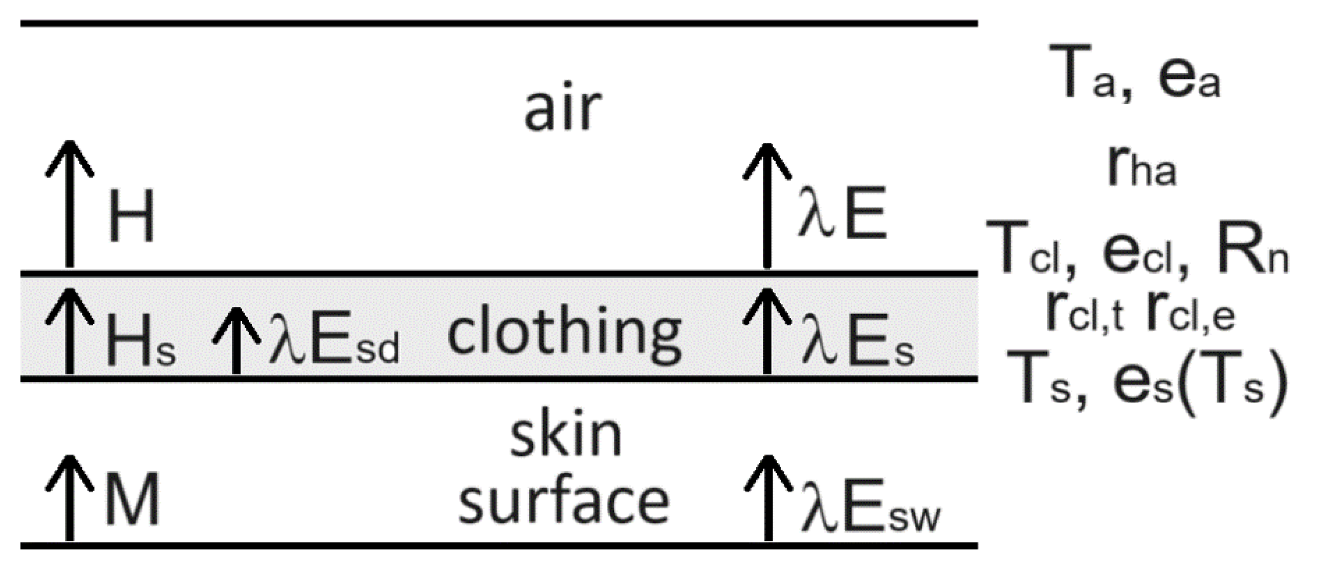
Clothing should be comfortable, that is, we should feel comfortable wearing it. This means that it must always remain dry, regardless of the rate of sweating, and we must not feel either an excess of heat or a lack of heat in it, regardless of our activity and the environmental thermal load. There is no such ideal clothing in reality, so the clothing parameters estimated with the model are the parameters of an imaginary clothing. A schematic diagram of the heat transports and state variables of the imaginary clothing is shown in
Figure 1.
2.1. Basic Equations
The environmental heat surplus or heat deficit strongly depends on the radiation conditions, so the radiation balance of the clothing surface is also a determining environmental factor. The two energy balances and the radiation balance can be written as follows:
where M is the metabolic heat flux density, W is the flux density of the work of the muscles used during the activity [
2], H
res is the respiration sensible heat flux density, λE
res is the respiration latent heat flux density, R
ni is the net isothermal radiation energy flux density on the surface of the clothing, S is the solar radiation energy flux density, α
c is the albedo of the clothing, ε
c is the emissivity of the clothing, ε
a is the emissivity of the troposphere and σ is the Stefan-Boltzmann constant. M is parameterized according to [
14]. Its parameterization is described in detail in the work of Kristóf et al. [
8].
2.2. Parameterizations
The following parametrizations were used to describe the heat transports in the model:
Skin surface evaporation (6a) is the sum of evaporation from dry skin and skin covered in sweat. In the dry skin evaporation formula (6b), T
S is given in °C (34 °C), while e
a is given in Pa [
15]. The rate of sweating (6c) cannot be simulated based on the description of physiological processes. There is a simple estimate, which is (6c), in which A
f is the surface of the human body, λ is the latent heat of evaporation and dm/dt is the loss of body weight caused by sweating, i.e. the amount of water sweated out per unit of time. This can easily be determined from the body mass and time values measured before and after the activity. The literature calls this λE
sw "regulatory sweating". The application of (6c) is challenging, but in our opinion it is the only reliable method for estimating the rate of sweating. The basic assumption of the model is that eq. (8) is valid. This is the guarantee that the clothing remains dry (there is neither convergence (clothing gets wet) nor divergence (clothing dries)), because we only feel comfortable in dry clothing. This makes sense, because wet clothing would sooner or later become uncomfortable due to its cooling effect. A
f was calculated by using the formula of Dubois and Dubois [
16].
2.3. The Clothing Evaporative Resistance Model
The two essential output variables of the clothing evaporation model are e
cl and r
cl,e. By combining (6a), (7) and (8), it is easy to express e
cl,
and since both λE
sd and λE
sw can easily be estimated based on the input meteorological and human (body mass, body length) variables, e
cl can be calculated with ease. It can also be seen that by applying (6), (7), (8) and (9), r
cl,e can also be expressed as follows:
The parametrization of r
Ha has already been described in several works [
5,
8]. The unit of r
cl,e is [s·m
−1], but in the literature there is also the [clo] unit for water vapor transport. 1 clo-e = 0.155 m
2·hPa·W
−1, based on which 1 clo-e = 0.155·(ρ·c
p/γ) = 0.155·(1.2·1004/0.65) = 287.3 s·m
−1.
2.4. The Clothing Thermal Resistance Model
The output variables of the clothing thermal resistance model are T
cl and r
cl,t. Let's express them! H
S can be expressed from (1) and described as
Here, the difference in human heat flux densities is denoted by Hu. By combining (2), (5), (8) and (11), we can write the following equation:
The final form of T
cl after substituting (3a) into (12) is:
Note that when estimating T
cl, we used both (1) (energy balance of skin surface under clothing) and (2) (energy balance of clothing surface), i.e., the magnitude of this temperature is influenced by both environmental and human factors. By combining (4) and (11), r
cl,t can be expressed,
Equations (13) and (14) are new equations and characterize the thermal properties of the clothing that creates thermal balance (neither excess of heat nor lack of heat) between the human body and its environment. Since it is clothing that creates heat balance, this clothing is imaginary. The unit of rcl,t is [s·m−1], but the [clo] unit is also used for heat transfer. 1 clo-t = 0.155 m2·°C·W−1, based on which 1 clo-t = 0.155·(ρ·cp) =0.155·(1.2·1004) = 186.7 s·m−1.
2.5. Operative Temperature Model
The operative temperature is a known heat load indicator. It is estimated as follows:
As we can see, it depends on environmental factors (air temperature, radiation and wind). Its dependence on human factors is negligible (it is hidden in the parameterization of rHa).
3. Location of Measurements and Observations, Tools Used
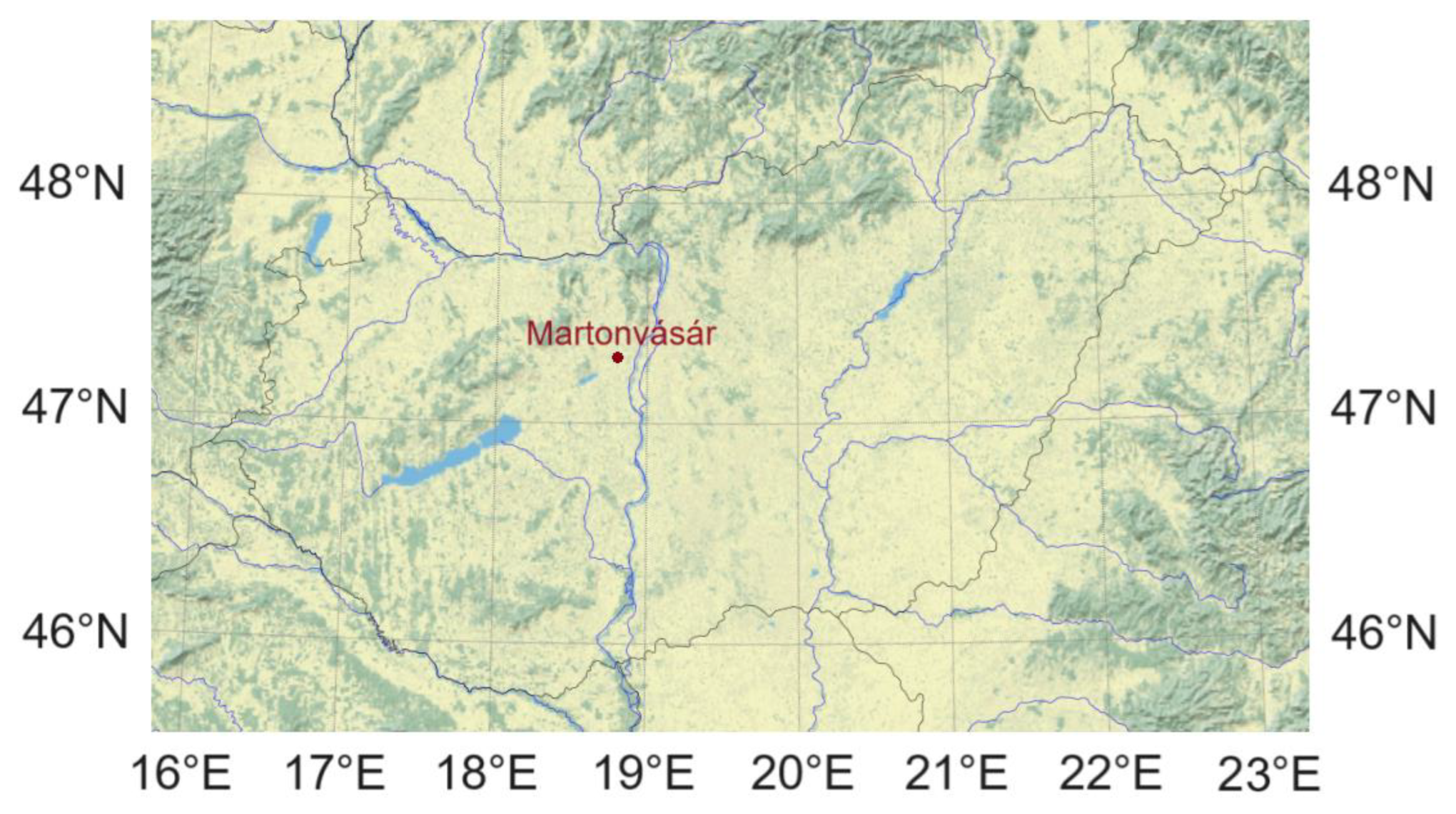
The location of the observations: Martonvásár, on the vineyard road starting next to the family house of the first author. This location made it possible to minimize the difference between the two times of weight measurement and the duration of the walk. The town Martonvásár is presented in
Figure 2 on a topographical map of Hungary.
The body mass was measured using an Orion digital weight meter, accuracy: 0.1 kg. When the mass values were read, the time was also recorded, to the minute. We estimated the duration of walking with two devices: an AppleWatch smartwatch and a JUNSO stopwatch, this was done for control purposes. Knowing the length of the road and the duration of the walk, it was also possible to estimate the average walking speed.
4. Data
Human and weather data were used.
4.1. Human Data
Human data provide information on 1) human state variables, 2) body mass immediately before and after walking, 3) the times of body mass measurements and thus the duration of observation, and 4) the duration of walking. The following human state variables are used: body mass (most important), body length, sex, age. These data of the observer are presented in
Table 1.
The observer was always on foot. Walking speeds varied between 1.1 and 1.7 ms−1.
4.2. Weather Data
The weather elements used to drive the model are: air temperature, air humidity, average wind speed, wind gust speed, cloud cover and relative sunshine duration. With the exception of the last two, all data were taken from the HungaroMet (Hungarian Meteorological Service Nonprofit Zrt.) website (
https://www.met.hu/en/idojaras/aktualis_idojaras/megfigyeles/) and transcribed into the database. The beeline distance between the HungaroMet automatic station and the location of the observations is less than 3 km. These data are 10-minute averages. The values of cloud cover and relative sunshine duration were estimated by the observer for the selected 10-minute time interval. Cloudiness is estimated visually in tenths. Global radiation is an hourly value expressed in Wm
-2 (Mihailović and Ács, 1985 [
17]) and refers to the hour interval in which the 10-minute observation took place. We performed a total of 115 observations in the period June 2, 2023 – March 9, 2024. The wheater elements observed ranged as follows: solar radiation varied between 0-870 Wm
-2, air temperature between -1-36 °C, average wind speed between 0.3-7.5 ms
−1, relative humidity between 34-100% and cloud cover between 0-1.
5. Results
Several results are presented and discussed. Since skin surface evaporation is a determining input variable, we analyzed its relationship with the rate of sweating, operative temperature and metabolic heat flux density. After that, we turned to analyzing the relationship between a) r
cl,t and λE
S, b) r
cl,t and T
cl, c) r
cl,e and λE
S and finally d) T
cl and T
o. It should be mentioned that the most important output variables of the model were listed for all 115 cases, they can be viewed in
Table S2 of the Supplementary material.
5.1. Sweating Rate and Skin Surface Evaporation: Dependence on M and To
We could see that skin surface evaporation is the sum of evaporation from dry skin and skin covered in sweat (eq. 6a). Our measurements and calculations provide insight into the relationship between these variables in the case of a walking individual. The average walking speed of the observer varied between 1.1 and 1.7 ms
−1. In this speed interval, the measured sweat rates varied between 0-0.8 kg/(30-45 minutes). The largest amount of water sweated out was 0.8 kg, in this case the rate of sweating was 0.8/(72 minutes). The latent heat flux density of sweating varied from 0 to 340 Wm
-2. In contrast, latent heat flux of evaporation from dry skin is 10-15 Wm
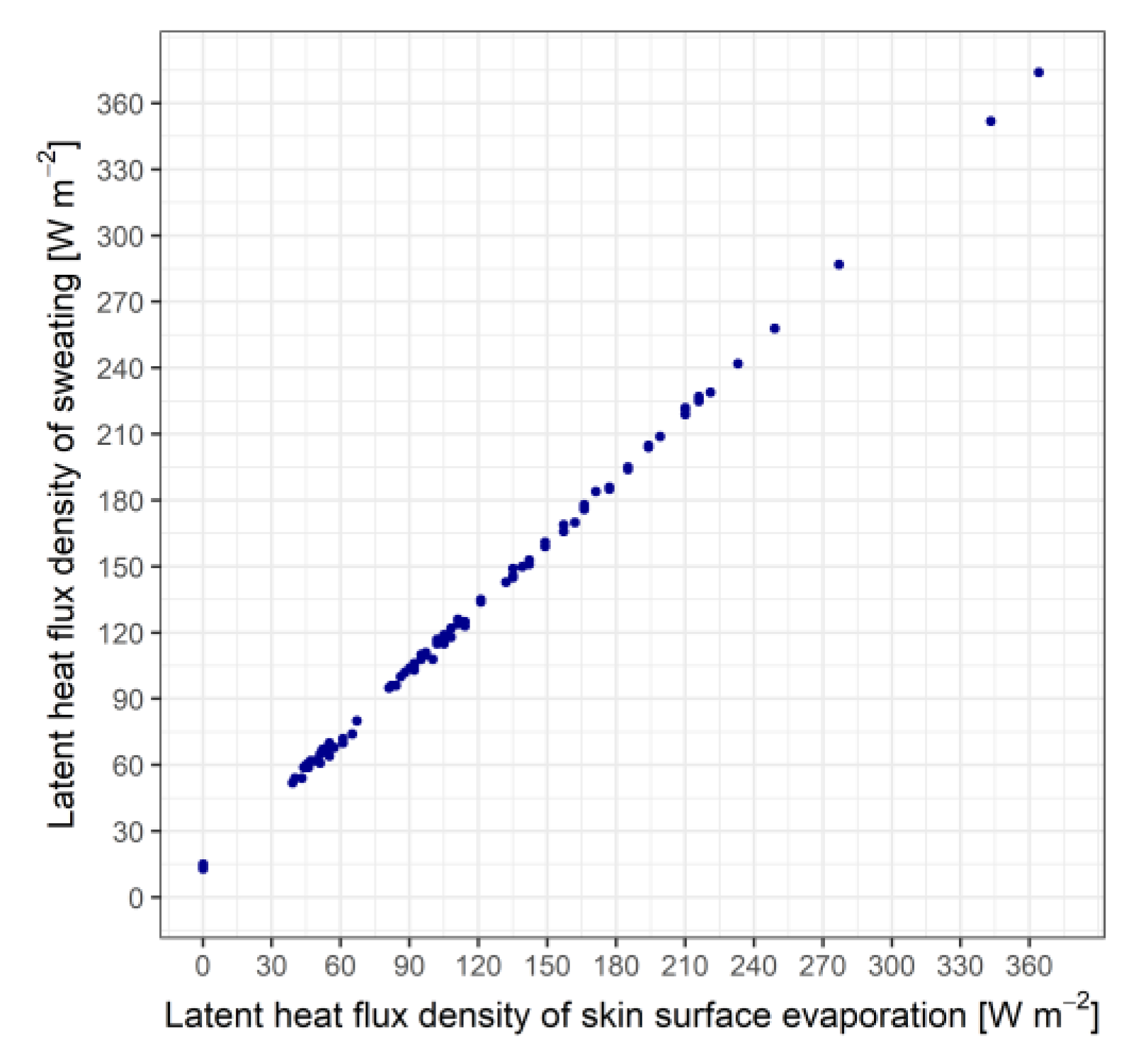
-2. λE
sw is the dominant component of λE
S, which can be seen in
Figure 3.
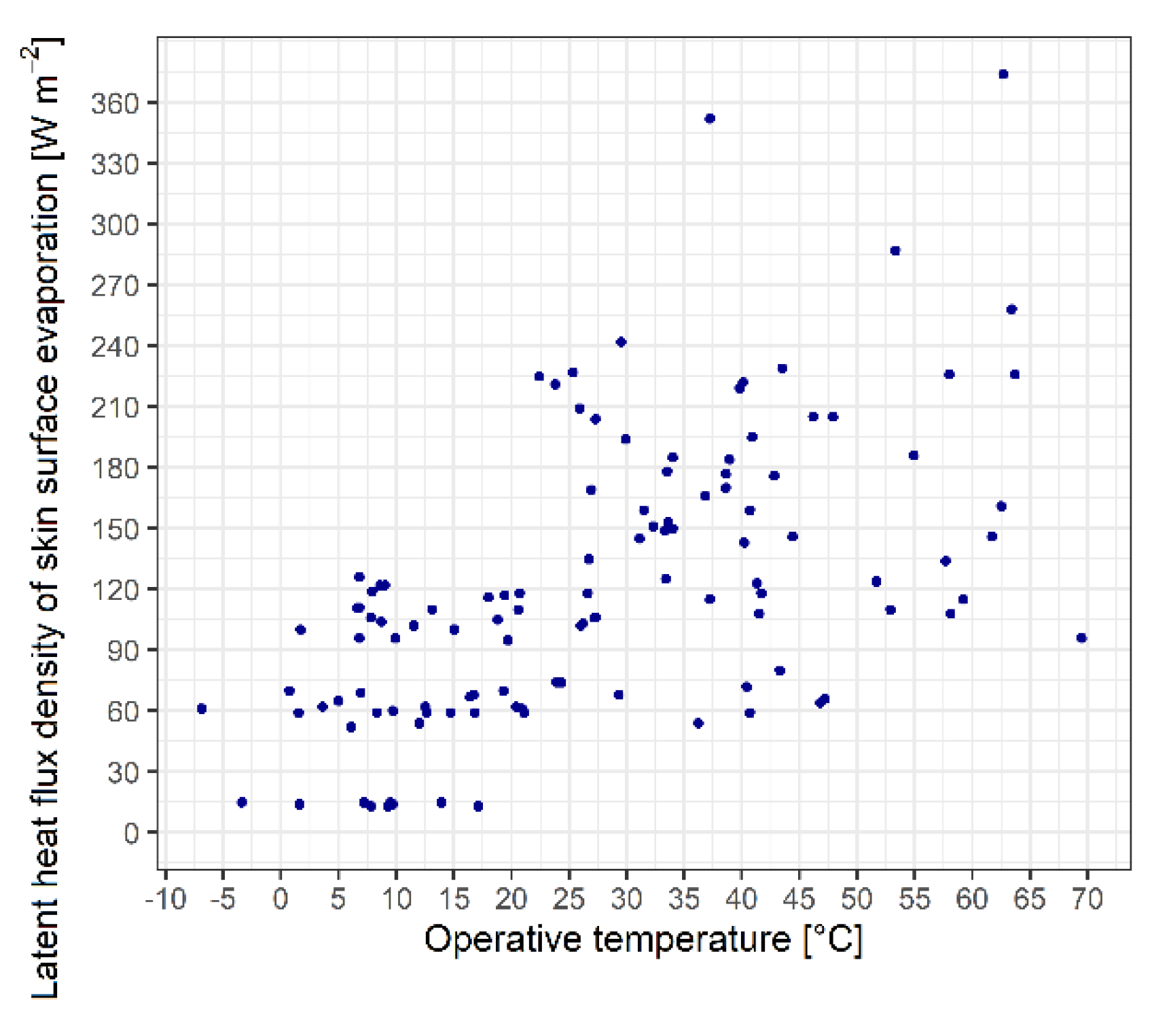
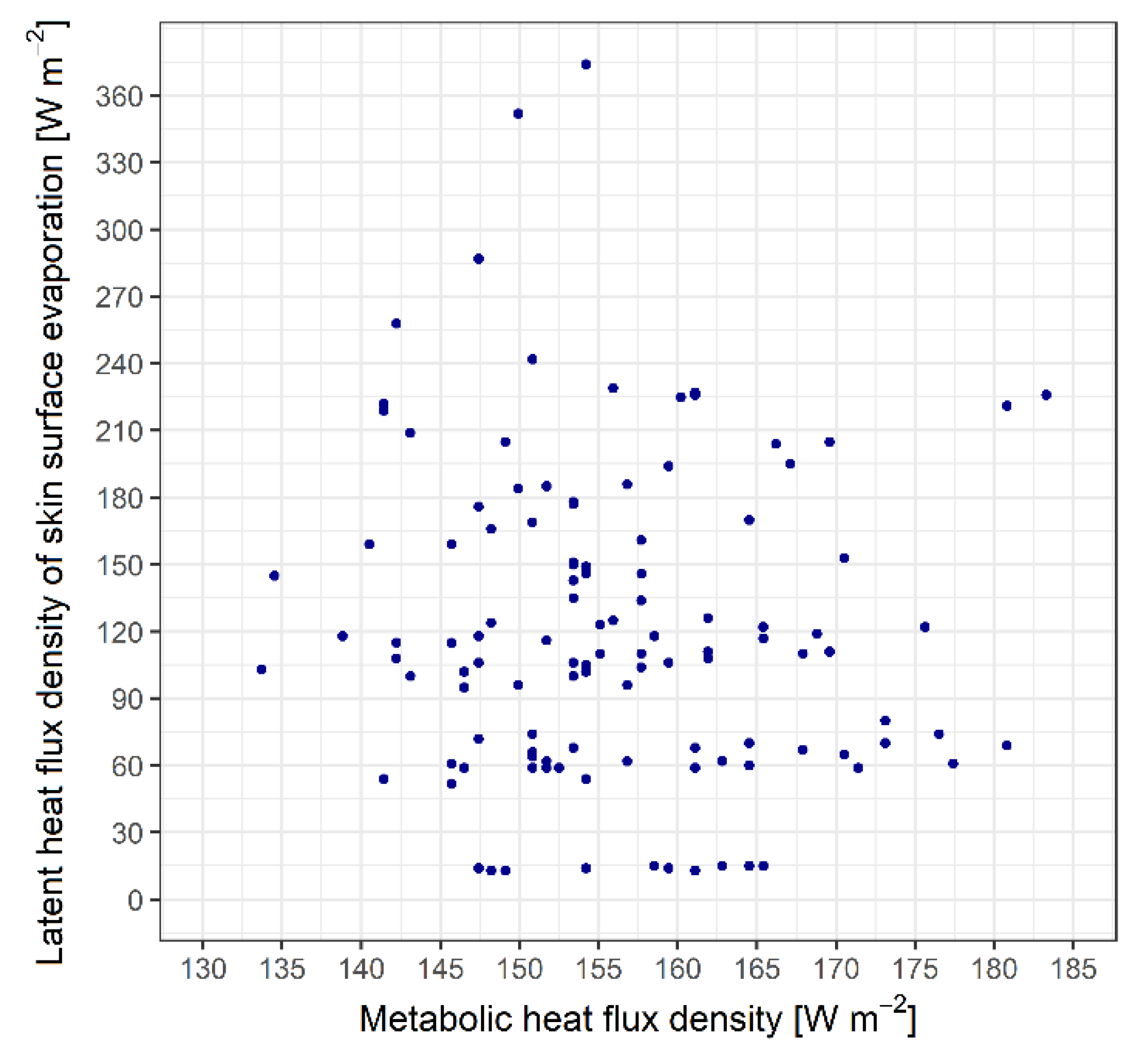
We can see that the λES – To relationship emerges more distinctively than the λES – M relationship, but it should be emphasized that To varied within much wider limits (-7 – 70 °C) than M (133-183 Wm-2). The large spread of points suggests that the variability of λES is influenced by many different and independent factors.
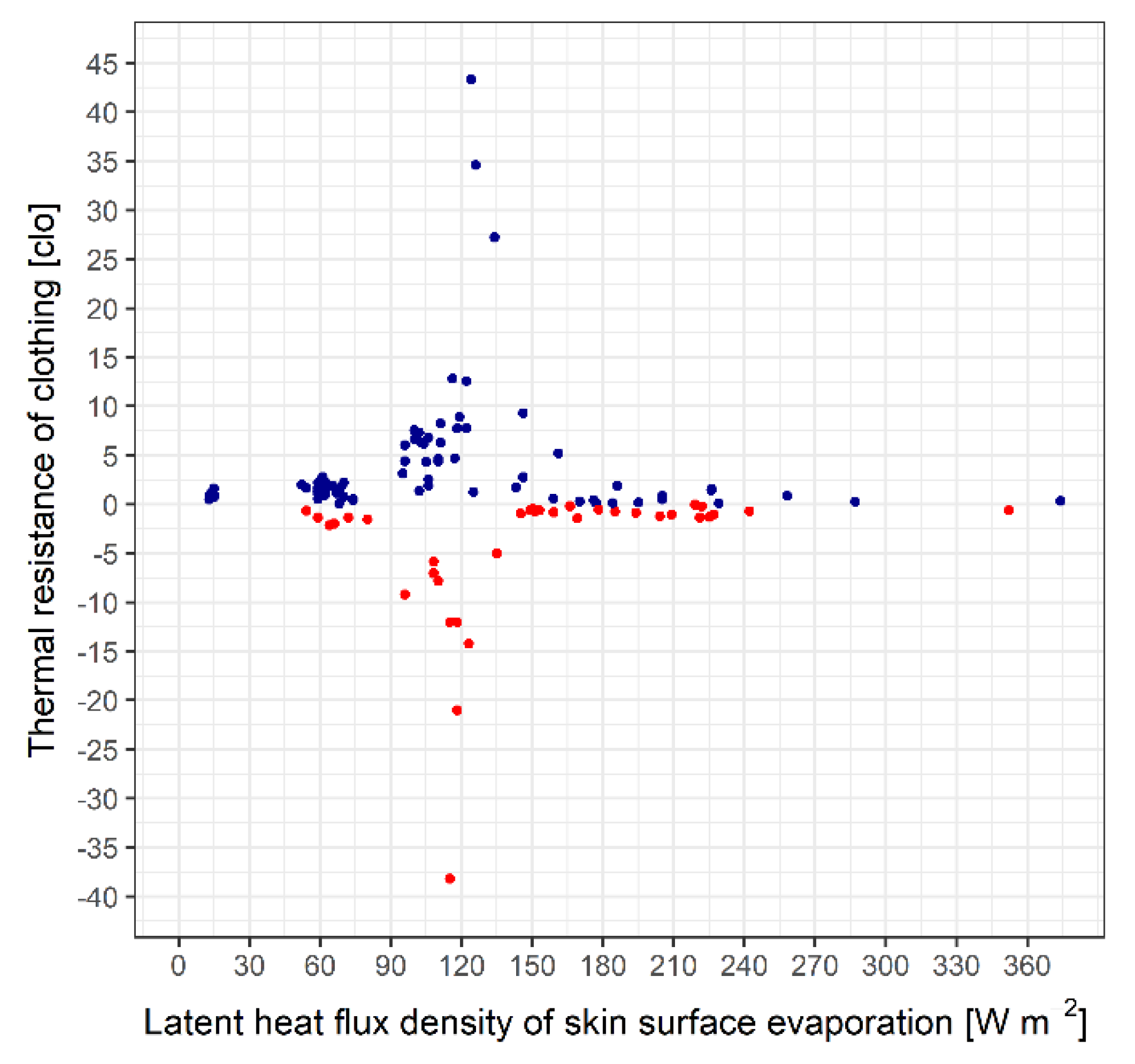
5.2. The Relationship between Clothing Thermal Resistance and Skin Surface Evaporation
The scatterplot of the relationship between the thermal resistance of clothing and the latent heat flux density of skin surface evaporation is presented in
Figure 6.
λES varied between wide limits (0-360 Wm-2), the obtained rcl,t value range was 0-43 clo-t. rcl,t strongly depends on λES. It can be noticed that rcl,t is close to 0 for very low (λES < 70 Wm-2) and very high (λES > 165 Wm-2) λES values. In the range 70 < λES < 165 Wm-2, the rcl,t values are greater than 3 clo-t in the vast majority of cases. It can also be noticed that in this range the value λES = 120 Wm-2 (in this case the rate of sweating is 0.2 kg/(35 minutes)) is the limiting value, separating the increasing and decreasing rcl,t values. It should be emphasized that these high rcl,t values are not physically based, but rather the consequence of the singularity of the method (eqs. (14) and (11)). Very high rcl,t values occur when Hu is close to 0. It is obvious that if Hu is close to 0 and greater than zero, then TS > Tcl (cases of environmental heat deficit), and conversely, if Hu is close to 0, but less than zero, then TS < Tcl (cases of environmental heat excess). The point Hu = 0 is the singularity point of the methodology (eq. (14)).
In the case of ambient heat deficit, rcl,t increases with increasing λES. In this case, the smallest rcl,t values are for λES = 0. These values were between 0.5 and 1.6 clo-t and, given the lack of heat, should be considered as physically based values. Note that minimal sweating (0.1 kg/(30 minutes)) significantly increases rcl,t values in the case of environmental heat deficit. In these cases, rcl,t can reach up to 2.5 clo-t.
In the case of environmental heat excess, rcl,t decreases with increasing λES. When the rate of sweating is 0.5 kg/(30 minutes), the rcl,t values are below 1 clo-t, which clearly shows that sweating can create a heat balance between the environment and the human body even in weather situations with a large excess of heat. Thus, for instance, for To = 43.5 °C, when λES = 229 Wm-2 (sweating rate 0.5 kg/(44 minutes), average walking speed 1.36 ms−1) rcl,t = 0.11 clo-t, which practically means thermal neutrality.
It’s to be mentioned that in cases of thermal comfort (rcl,t close to 0 clo-t), the absolute value of the (TS -- Tcl) difference is very small (0.8-2 °C), completely regardless of which λES range we are talking about.
The described results refer to the blue points in the figure, in these cases the method can be used, that is r
cl,t > 0 clo-t. In the case of the red points shown in
Figure 6, the method cannot be applied because r
cl,t < 0 clo-t. We will deal with the analysis of non-applicable cases separately in
Section 5.6.
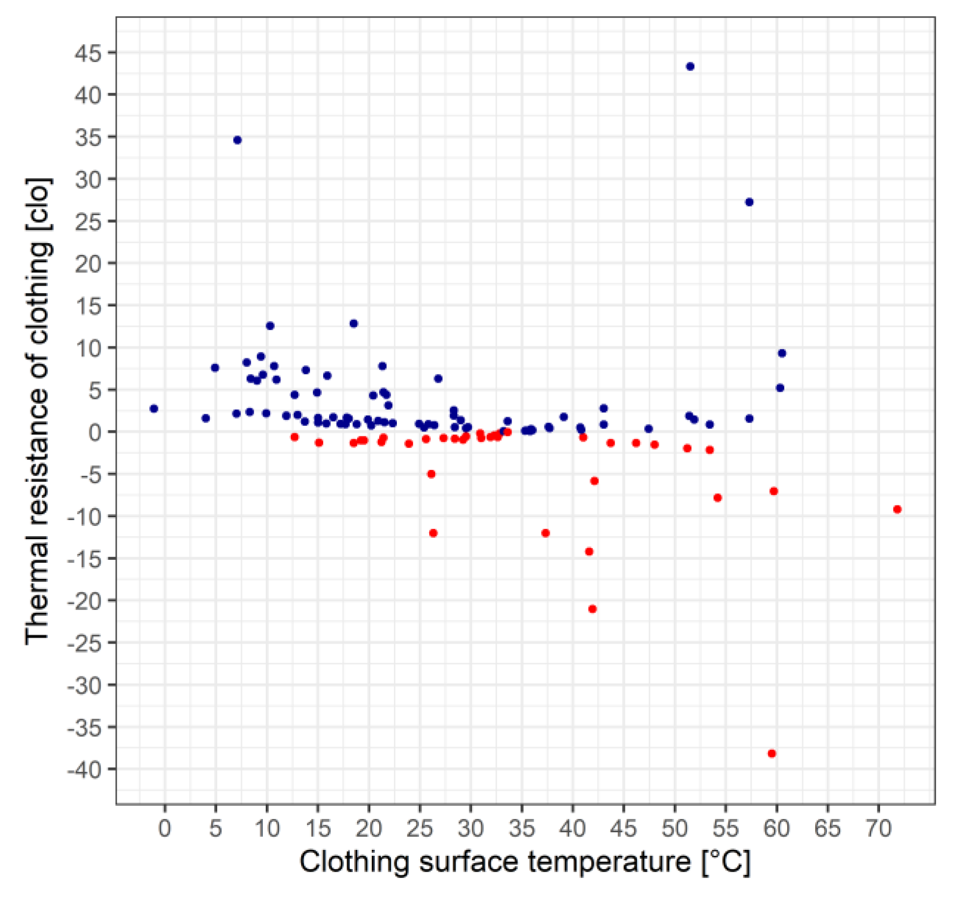
5.3. The Relationship between Thermal Resistance and Surface Temperature of Clothing
The scatterplot of the relationship between clothing thermal resistance and surface temperature is presented in
Figure 7.
The large scatter of the points is caused by the mentioned methodological singularity (Hu → 0). Therefore, we will only look at rcl,t values below 4 clo-t (the rcl,t = 4 clo-t value can be taken as the upper limit of the heat deficit in the lowland regions of Hungary). In this case, the characteristics of the rcl,t – Tcl relationship can already be clearly recognized. The rcl,t – Tcl relationship can be divided into 3 ranges: 1) Tcl is much smaller than TS, 2) Tcl is around TS and 3) Tcl is much larger than TS. The main characteristic of the 1st range is the lack of environmental heat, accordingly rcl,t gradually increases as Tcl decreases. This change is clearly visible. In conditions close to thermal neutrality, rcl,t values are by definition close to 0 clo-t. Here there is also a point with rcl,t = 1.3 clo-t, which is large despite the small (TS – Tcl) difference (0.4 °C), because Hu is very small, it is only 2.2 Wm-2. This result does not reflect the real thermal state, it is caused by the singularity of the methodology. In the 3rd range, there are smaller or larger excesses of heat, during which the amount of sweating can also be smaller or larger. If the excess of heat is extremely high and so is the rate of sweating, then rcl,t → 0 clo-t. If, on the other hand, there is less sweating in such cases, Tcl and rcl,t will also be higher. If Hu becomes positive due to a small amount of sweating, then the method is unapplicable. If the environmental heat excess is smaller and the amount of sweating is also smaller, the rcl,t values change similarly as in the previous case. Given that we are talking about excess heat conditions, rcl,t values greater than 1.2-1.4 clo-t cannot be considered as physically based, but rather as caused by the singularity of the method.
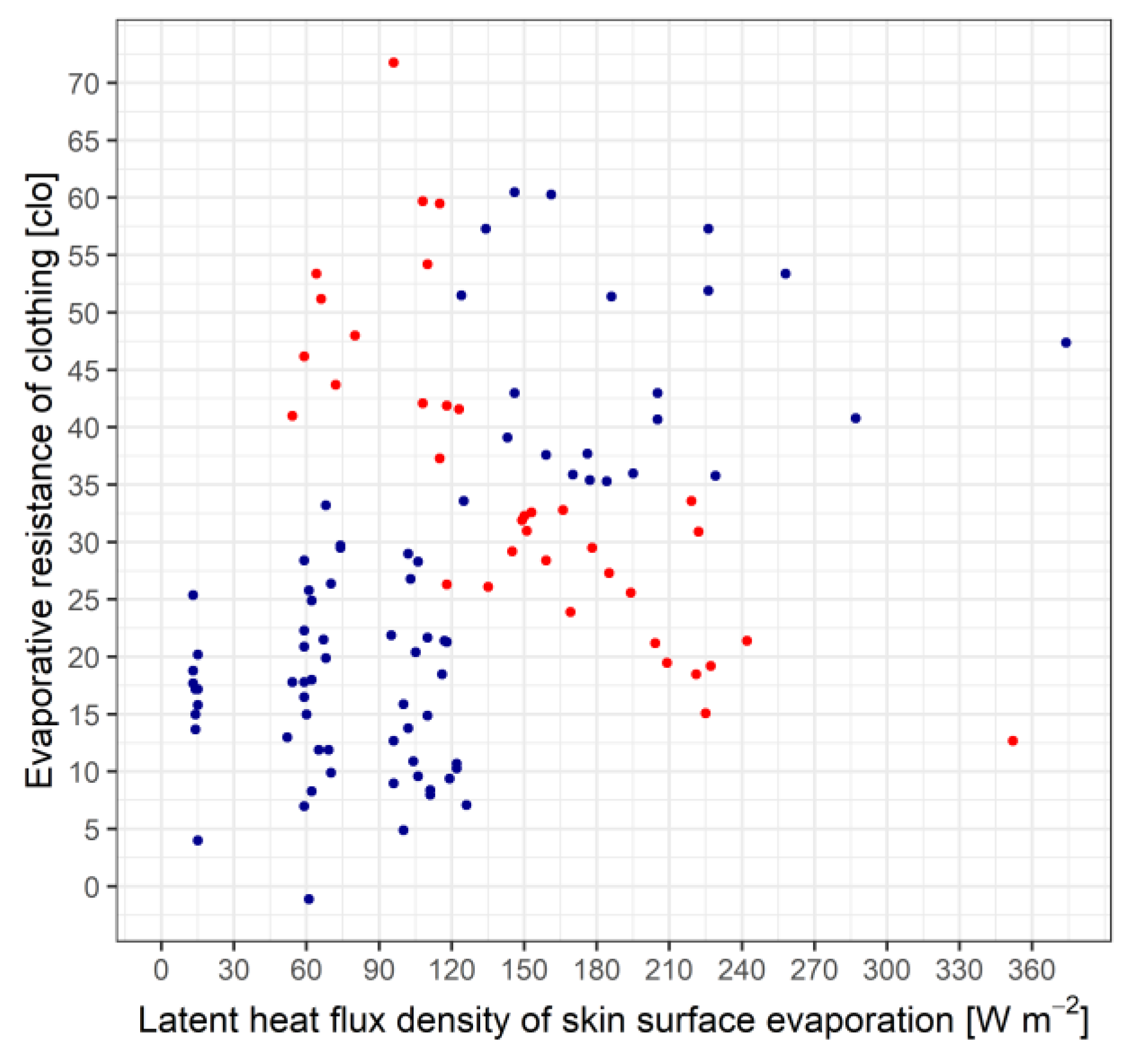
5.4. The Relationship between the Clothing Evaporative Resistance and Skin Surface Evaporation
The scatterplot of the relationship between the evaporative resistance of clothing and the latent heat flux density of skin surface evaporation is presented in
Figure 8.
The rcl,e – λES relationship is determined by the requirements (eqs. (8) and (10)) for comfortable clothing. As we can see, rcl,e decreases exponentially with increasing λES. The rcl,e values varied between 0.1 (for λES = 353 Wm-2) and 21 (λES = 14 Wm-2, there is no sweating) clo-e. If there is already sweating (λES = 60-80 Wm-2, sweating rate is 0.1 kg/(30 minutes)), the rcl,e values are around 4-5 clo-e. The relationship between rcl,e – ecl is also exponential, like the relationship between rcl,e and λES, so it is neither illustrated nor analyzed.
5.5. The Relationship between Operative Temperature and Clothing Surface Temperature
In addition to the estimation of Hu, the estimation of T
cl is also important for the success of the method. In the absence of direct verification, T
cl was compared with T
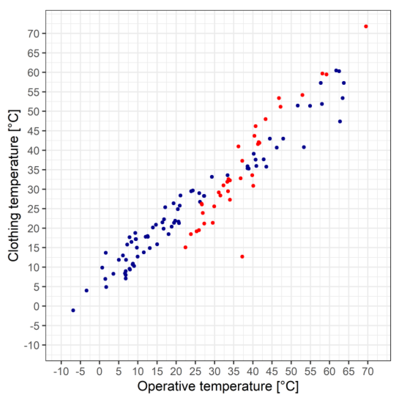
o. The scatterplot of the relationship between clothing surface temperature and operative temperature is presented in
Figure 9.
The relationship between Tcl and To is linear, despite the scatter of points. Two ranges can be recognized: 1) in the range Tcl < TS the Tcl values are larger than the To values, and 2) in the range Tcl > TS the Tcl values are generally somewhat smaller than the To values.
5.6. Applicability of the Model
The model has limited applicability. Three cases can be distinguished: 1) the model cannot be applied because the values of r
cl,t < 0, 2) the model simulates large, non-physically based r
cl,t values (methodological singularity) and 3) the model simulates real, physically based r
cl,t values. All these cases can be seen in
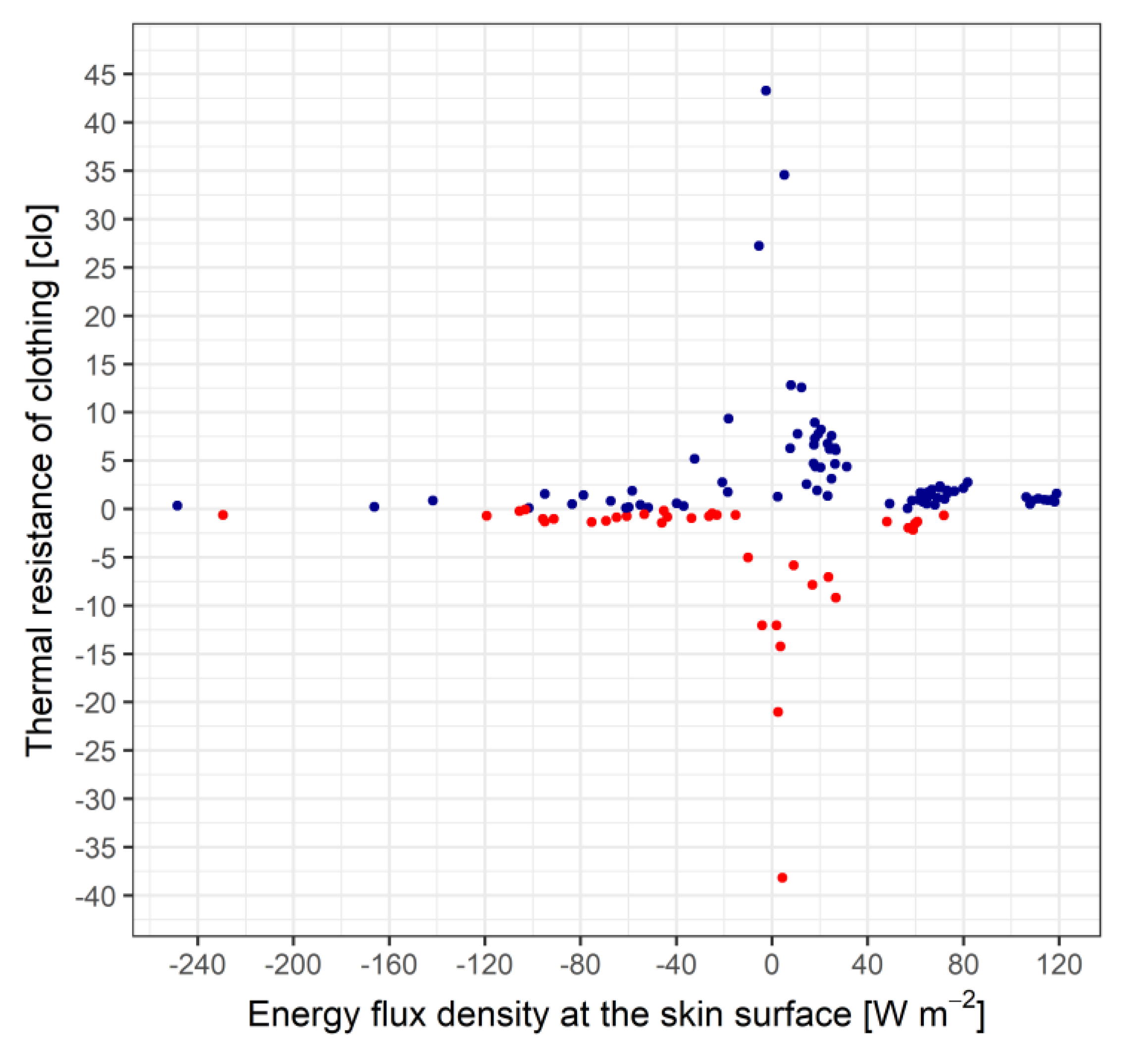
Figure 10, where the scatterplot of the r
cl,t – Hu relationship is shown.
Red points represent not applicable cases (case 1). The blue points with a very high r
cl,t values (case 2) are the consequence of the methodological singularity, they are mostly in the range -40 < Hu < 40 Wm
-2. The physically based r
cl,t values (case 3) are in the most negative (the latent heat flux density of the sweated water is much higher than the metabolic heat flux density and there is a large heat surplus) and the most positive (no sweating and there is a large heat deficit) Hu value ranges. In this figure, it is difficult to recognize the points representing the state of thermal neutrality (r
cl,t is close to 0 clo and the temperature difference (T
S – T
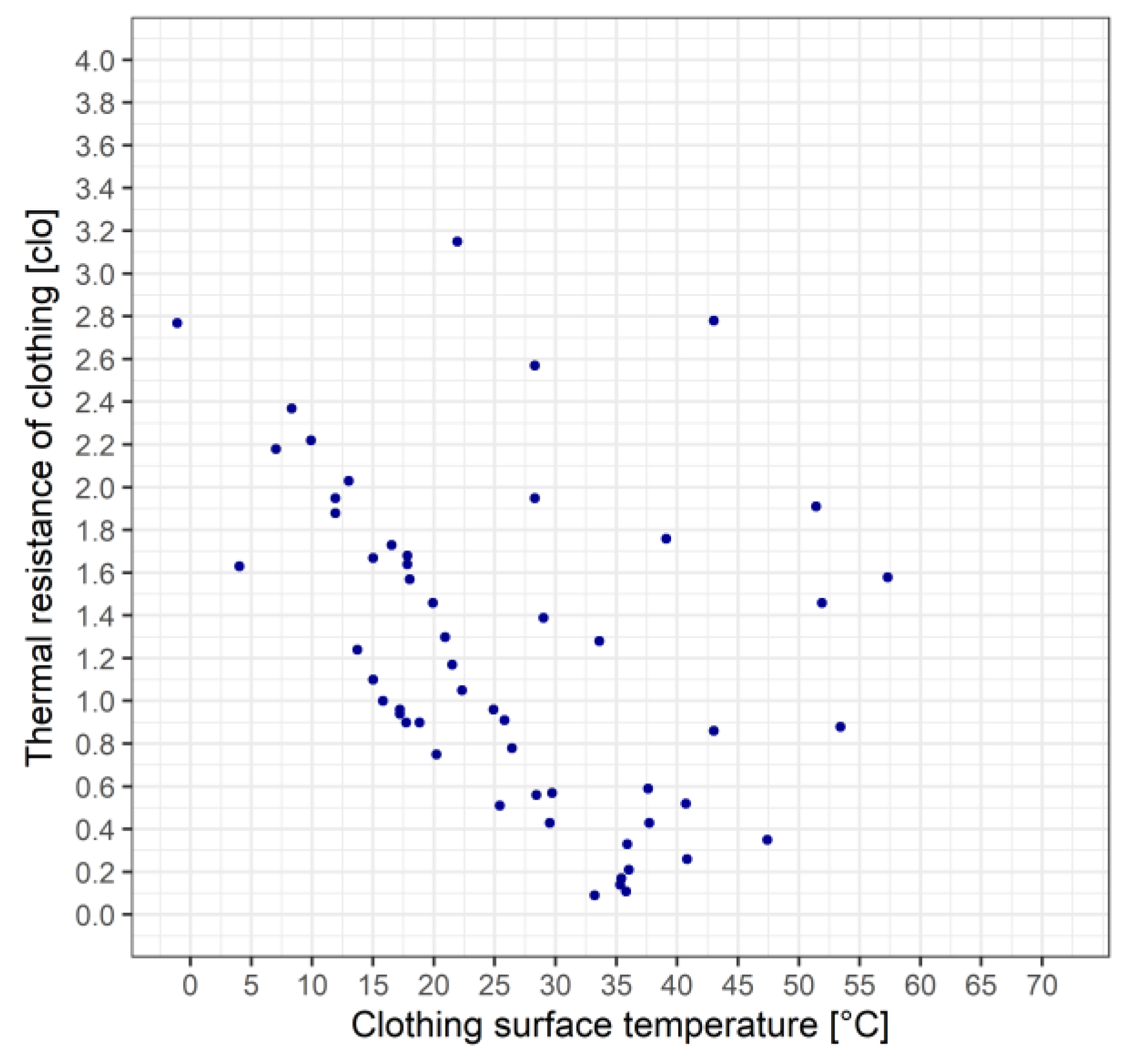
cl) is small, a few °C). These cases can be seen in
Figure 11 for values of T
cl, which are close to T
S.
In summary: the method performs well in the range of thermal neutrality, as well as when 1) the environmental heat surplus is high and the rate of sweating is high, 2) the environmental heat deficit is high and there is no sweating.
6. Discussion
Our measurements and analyzes showed that the model is suitable for simulating and characterizing the individual human climate. Today, there are no individual human climate descriptions, only attempts [
6] that are similar to this one. The reasons for this are as follows: 1) the concept of the "standard/average" person has spread in human meteorological studies. There is no simulation for individuals, so that human variability does not have to be dealt with, and it is also important that conducting longitudinal measurements with individuals is a very tedious and complex task. 2) We characterize a human climate instead of a human thermal climate by expanding the concept of comfortable clothing. Clothing is comfortable when it is dry and thermally neutral. The imaginary clothing used in the model fulfills these two conditions. The condition of thermal neutrality was achieved by applying the energy balance equation at the clothing-air environment interface, and the condition of dry clothing is achieved by equating the latent heat flux densities leaving the skin surface and the clothing surface. Thus, the clothing was characterized not only from a thermal point of view, but also from a moisture point of view, accordingly, the model consists of a thermal and an evaporative module. With the addition of the evaporative module and its coupling to the thermal module, we obtained a new clothing resistance model.
Which are the most important results that can characterize the simulated individual human climate? We would highlight three results that refer to the environmental heat surplus, the environmental heat deficit, and thermal neutrality. In the case of high thermal loads, the r
cl,t values were between 0.1-0.5 clo-t, while the r
cl,e values were between 0.4-0.8 clo-e. The values of r
cl,t and r
cl,e close to 0 were caused by intense sweating (λE
sw > 200 Wm
-2). The former models [
1,
5] - as they did not simulate the process of sweating - were not applicable in these heat excess situations. In heat-deficient situations, the amount of sweating decreases, so the r
cl,e values increase, and they are the highest when there is no sweating and the evaporation from the skin surface is equal to the evaporation from dry skin. In such cases, r
cl,e values were around 20-21 clo-e (λE
sd 10-15 Wm
-2), r
cl,t values varied between 0.5-1.6 clo-t. It should be mentioned that the average winter r
cl,t values are around 1.3-1.8 clo-t [
4,
5] In conditions close to thermal neutrality (T
cl values are close to T
S), we can sweat while walking - especially if we walk at a faster pace. Thus, when r
cl,t values were 0.1-0.4 clo-t, the corresponding r
cl,e values were 0.8-3 clo-e. Sweating is considered to be natural when we walk for longer distances at higher speeds (> 1.1 ms
−1).
These parameters characterize imaginary clothing for an individual (
Table 1). How close are the parameters of the imagined clothing to the parameters of real clothing? In this regard, we would like to make a comment about the r
cl,e values. We observed that the t-shirt worn was always wet when sweating, this was visible. This means that the sweated water flux density is convergent, that is, the clothing absorbs water, even if the amount is negligible. Real and imaginary clothing differ in this, that is, the r
cl,e values of the real clothing are obviously larger than the r
cl,e values of the imaginary clothing. Therefore, the r
cl,e values of the imagined clothing are to be considered as lower limit values.
One of the key variables in the model is the rate of sweating. λE
sw determines both the thermal and evaporative climate of an individual. In the cold season, λE
sw is minimal, close to zero; in the warm season it can be extremely high (200-300 Wm
-2), it depends not only on the environmental heat load, but also on the activity. In our study, the λE
sw – M dependence is weak (
Figure 5), as M varied between narrow limits (135 – 189 Wm
-2), while the variability of the environmental heat load (-7 °C < T
o < 70 °C) was large. The relation of λE
sw to M is of decisive importance, which can be seen from equations (11) and (14) of the model. If Hu is close to 0 (there is a mathematical singularity at the point Hu = 0), the r
cl,t values are unrealistically high, that is, they are not physically based. Little is known about the interpersonal variability of sweating [
18]. To establish this, several similar longitudinal experiments would be needed, which goes beyond the framework of an individual project.
The model can be applied to all activities if M and λE
sw characterizing the activity are known. In our previous models, we did not estimate sweating, the activity was walking at a speed of 1.1 ms
−1 [
4,
5,
6,
7,
8]. Examining the applicability of the model in the case of lying down and running is one of the important goals of our future research. We can say that the model can be used in any climate, weather and activity. The determinant physiological variables of the model are M and λE
sw, the relationship between which is unknown in many respects.
7. Conclusions
In this study, we continued the development of the clothing resistance model type. Until now, these models [
4,
5,
6,
7,
8] have only been used in the winter season and in cold climates, because the determination of sweating was omitted when estimating r
cl,t. We changed this concept and characterized both the thermal and moisture climates of a person by determining sweating. Since sweating is individual-specific, the model can be applied individually. Our main conclusions are as follows: 1) the human climate can be characterized not only from a thermal point of view, but also from a moisture point of view. Knowledge of sweating is necessary not only to estimate r
cl,e, but also r
cl,t. 2) Sweating is the determining variable in the estimation of both r
cl,t and r
cl,e, but little is known about its interpersonal variability. 3) The applicability of the model strongly depends on the relationship between λE
sw and M, the human variability of which we know little about.
Supplementary Materials
The following supporting information can be downloaded at the website of this paper posted on Preprints.org.
Author Contributions
Conceptualization, F.Á.; methodology, F.Á.; software, F.Á. and E.K.; validation, F.Á.; formal analysis, F.Á.; investigation, F.Á.; resources, F.Á.; data curation, F.Á. and E.K.; writing—original draft preparation, F.Á.; writing—review and editing, F.Á. and E.K.; visualization, E.K.; supervision, F.Á. E.K.; project administration, F.Á.; funding acquisition, F.Á. All authors have read and agreed to the published version of the manuscript.
Funding
“This research received no external funding”. Online publication cost has been funded by Publisher.
References
- Auliciems, A.; de Freitas, C.R. Cold Stress in Canada. A Human Climatic Classification. Int. J. Biometeorol. 1976, 20, 287–294. [Google Scholar] [CrossRef] [PubMed]
- Auliciems, A.; Kalma, J.D. A Climatic Classification of Human Thermal Stress in Australia. J. Appl. Meteorol. (1962-1982) 1979, 18, 616–626. [Google Scholar] [CrossRef]
- Burton, A.C.; Edholm, O.G. Man in a Cold Environment. Edward Arnold Ltd., London, 1955, 273 pp.
- Ács, F.; Zsákai, A.; Kristóf, E.; Szabó, A.I.; Breuer, H. Carpathian Basin climate according to Köppen and a clothing resistance scheme. Theor. Appl. Climatol. 2020, 141, 299–307. [Google Scholar] [CrossRef]
- Ács, F.; Zsákai, A.; Kristóf, E.; Szabó, A.I.; Breuer, H. Human thermal climate of the Carpathian Basin. Int. J. Climatol. 2021, 41, E1846–E1859. [Google Scholar] [CrossRef]
- Ács, F.; Kristóf, E.; Zsákai, A. Individual local human thermal climates in the Hungarian lowland: Estimations by a simple clothing resistance-operative temperature model. Int. J. Climatol. 2023, 43, 1273–1292. [Google Scholar] [CrossRef]
- Ács, F.; Szalkai, Z.; Kristóf, E.; Zsákai, A. Thermal Resistance of Clothing in Human Biometeorological Models. Geogr Pannonica 2023, 27, 83–90. [Google Scholar] [CrossRef]
- Kristóf, E.; Ács, F.; Zsákai, A. On the Human Thermal Load in Fog. Meteorology 2024, 3, 83–96. [Google Scholar] [CrossRef]
- Yan, Y.Y.; Oliver, J.E. The Clo: A Utilitarian Unit to Measure Weather/Climate Comfort. Int. J. Climatol. 1996, 16, 1045–1056. [Google Scholar] [CrossRef]
- Parsons, R.A. , 1997: 1997 ASHRAE Handbook, Chapter 8 (Thermal Comfort), Evaporative Heat Loss from Skin, 8.3 pp.
- Rovelli, C. Helgoland: Making Sense of the Quantum Revolution. Park Kiadó, Budapest, 2022, 269 pp. ISBN: 978-963-355-725-9. (in Hungarian).
- Campbell, G.S.; Norman, J. An Introduction to Environmental Biophysics; 2nd edition; Springer: New York, 1997; ISBN 978-0-387-94937-6. [Google Scholar]
- Katić, K.; Li, R.; Zeiler, W. Thermophysiological Models and Their Applications: A Review. Build. Environ. 2016, 106, 286–300. [Google Scholar] [CrossRef]
- Weyand, P.G.; Smith, B.R.; Puyau, M.R.; Butte, N.F. The mass-specific energy cost of human walking is set by stature. J. Exp. Biol. 2010, 213, 3972–3979. [Google Scholar] [CrossRef] [PubMed]
- Fanger, P.O. Thermal comfort: analysis and applications in environmental engineering. PhD Thesis, Danmarks tekniske højskole, Danish Technical Press, Copenhagen, 1970; p. 244, ISBN: 8757103410 9788757103410. [Google Scholar]
- Dubois, D.; Dubois, E.F. The Measurement of the Surface Area of Man. Archives of Internal Medicine 1915, XV, 868–881. [Google Scholar] [CrossRef]
- Mihailović, D.T.; Ács, F. Calculation of daily amounts of global radiation in Novi Sad. Időjárás 1985, 89, 257–261. (In Hungarian) [Google Scholar]
- Lim, C.L. Fundamental Concepts of Human Thermoregulation and Adaptation to Heat: A Review in the Context of Global Warming. Int. J. Environ. Res. Public Health 2020, 17, 7795. [Google Scholar] [CrossRef]
Figure 1.
Heat and moisture transports and state variables that characterize imaginary clothing. H - sensible heat flux density between the clothing surface and the air, λE - latent heat flux density between the clothing surface and the air, Ta - air temperature, ea - partial water vapor pressure of the air, Tcl - temperature of the clothing surface, ecl - partial water vapor pressure on the clothing surface, Rn - radiation balance of the clothing surface, rHa - aerodynamic resistance to heat transport between the clothing surface and the air, HS - sensible heat flux density between the skin surface and clothing, λES – latent heat flux density of skin surface evaporation, λEsd – latent heat flux density of dry skin surface evaporation between the skin and clothing, λEsw - the latent heat flux density of sweating, TS - the temperature of the skin surface (34 °C), eS(TS) - the water vapor pressure at saturation at TS temperature, rcl,t - the thermal resistance of the clothing, rcl,e - the evaporative resistance of the clothing and M - metabolic heat flux density.

Figure 2.
Martonvásár (47.31° N, 18.79° E), the location of the observations and topographical map of Hungary (Central Europe).
Figure 2.
Martonvásár (47.31° N, 18.79° E), the location of the observations and topographical map of Hungary (Central Europe).
Figure 3.
The relationship between the latent heat flux density of skin surface evaporation and the latent heat flux density of sweating for a walking person. Average walking speed varied between 1.1 and 1.7 ms
−1. The sweating rate depends on both human (for instance, M) and environmental (for instance, T
o, which provides information on the integrated thermal load of the environment) factors. The point clouds characterizing the relationship between λE
S and T
o and λE
S and M can be seen in
Figure 4 and
Figure 5, respectively.
Figure 4.
Scatterplot of the relationship between skin surface evaporation and operative temperature in the case of a walking observer. Observation period: June 2, 2023 -- March 9, 2024.
Figure 4.
Scatterplot of the relationship between skin surface evaporation and operative temperature in the case of a walking observer. Observation period: June 2, 2023 -- March 9, 2024.
Figure 5.
Scatterplot of the relationship between skin surface evaporation and metabolic heat flux density in the case of a walking observer. Average walking speed interval: 1.1-1.7 ms−1, observation period: June 2, 2023 -- March 9, 2024.
Figure 5.
Scatterplot of the relationship between skin surface evaporation and metabolic heat flux density in the case of a walking observer. Average walking speed interval: 1.1-1.7 ms−1, observation period: June 2, 2023 -- March 9, 2024.
Figure 6.
Scatterplot of the relationship between the clothing thermal resistance and skin surface evaporation. Blue points: the method is applicable (rcl,t > 0), red points: the method is unapplicable (rcl,t < 0). .
Figure 6.
Scatterplot of the relationship between the clothing thermal resistance and skin surface evaporation. Blue points: the method is applicable (rcl,t > 0), red points: the method is unapplicable (rcl,t < 0). .
Figure 7.
Scatterplot of the relationship between the clothing thermal resistance and surface temperature. Blue points: the method is applicable (rcl,t > 0), red points: the method is unapplicable (rcl,t < 0).
Figure 7.
Scatterplot of the relationship between the clothing thermal resistance and surface temperature. Blue points: the method is applicable (rcl,t > 0), red points: the method is unapplicable (rcl,t < 0).
Figure 8.
Scatterplot of the relationship between the clothing evaporative resistance and latent heat flux density of skin surface evaporation. Blue points: the method is applicable (rcl,t > 0), red points: the method is unapplicable (rcl,t < 0).
Figure 8.
Scatterplot of the relationship between the clothing evaporative resistance and latent heat flux density of skin surface evaporation. Blue points: the method is applicable (rcl,t > 0), red points: the method is unapplicable (rcl,t < 0).
Figure 9.
Scatterplot of the relationship between the clothing surface temperature and operative temperature. Blue points: the method is applicable (rcl,t > 0), red points: the method is unapplicable (rcl,t < 0).
Figure 9.
Scatterplot of the relationship between the clothing surface temperature and operative temperature. Blue points: the method is applicable (rcl,t > 0), red points: the method is unapplicable (rcl,t < 0).
Figure 10.
Scatterplot of the relationship between the clothing thermal resistance and the energy flux density at the skin surface.
Figure 10.
Scatterplot of the relationship between the clothing thermal resistance and the energy flux density at the skin surface.
Figure 11.
The scatterplot of the relationship between the clothing thermal resistance and the clothing surface temperature in the range of rcl,t < 0.8 clo.
Figure 11.
The scatterplot of the relationship between the clothing thermal resistance and the clothing surface temperature in the range of rcl,t < 0.8 clo.
Table 1.
Human state variables and basal metabolic heat flux density of the person conducting observations.
Table 1.
Human state variables and basal metabolic heat flux density of the person conducting observations.
| Person |
Sex |
Age[years] |
Body mass [kg] |
Body length [cm] |
Basal metabolic heat flux density [Wm−2] |
| the observer |
male |
68 |
89.0 |
190 |
40.8 |
|
Disclaimer/Publisher’s Note: The statements, opinions and data contained in all publications are solely those of the individual author(s) and contributor(s) and not of MDPI and/or the editor(s). MDPI and/or the editor(s) disclaim responsibility for any injury to people or property resulting from any ideas, methods, instructions or products referred to in the content. |
© 2024 by the authors. Licensee MDPI, Basel, Switzerland. This article is an open access article distributed under the terms and conditions of the Creative Commons Attribution (CC BY) license (http://creativecommons.org/licenses/by/4.0/).
