Preprint

Article

Navigating the Labyrinth of the Mind: Exploring Brain Models Through Complex Differential Equations

Altmetrics

Downloads

Views

Comments

Richard Murdoch Montgomery^*

This version is not peer-reviewed

This preprints belongs to the Topic

Advances in Nonlinear Dynamics: Methods and Applications

Submitted:

07 June 2024

Posted:

07 June 2024

You are already at the latest version

Alerts

Abstract

The endeavor to decode the brain's intricate architecture and its multifaceted functions has propelled scientists into the domain of complex differential equations, aiming to construct a computational framework capable of representing its uncountable intricacies. This article delves into the sophisticated and daunting task of modeling the brain, a system of seemingly uncountable coupled differential equations, each symbolizing the vast array of interconnected neural pathways and processes. We discuss the current limitations of computational resources and the significant challenges faced in accurately capturing the non-linear, high-dimensional, and plastic nature of neural dynamics. Despite these challenges, we explore the progressive strides in computational neuroscience that lay the groundwork for partial models, offering insights into the brain's localized circuits and broader network interactions. These models serve as pivotal stepping stones towards a more comprehensive understanding, which is incrementally built upon by interdisciplinary approaches, leveraging advancements in neuroimaging, data analysis, and theoretical biology. Looking ahead, the article speculates on the potential paradigm shifts that could arise from breakthroughs in computational technology, such as quantum computing, that may one day enable the simulation of the brain in its entirety. The article ultimately paints a picture of cautious optimism, where each incremental discovery is a valuable piece of the grand puzzle, bringing us closer to the epochal goal of comprehensively modeling the human brain.

Keywords:

Subject: Biology and Life Sciences - Biophysics

1. Introduction

The human brain, often compared to a dense forest of neural complexity, has fascinated scientists for centuries. The groundbreaking work of Hodgkin and Huxley in 1952 helped us understand the electrical properties of neurons, while Hebb’s 1949 concept of neural networks laid the foundation for our knowledge of learning and memory. These early studies set the stage for deeper exploration into the brain’s structure and function.

Advancements in neuroimaging and computational modeling brought new insights into how the brain processes information. For instance, the pioneering work of Hubel and Wiesel in 1962 revealed how the brain handles visual information, showing the intricate patterns of receptive fields and neural circuits. Building on this, Felleman and Van Essen in 1991 mapped the cerebral cortex’s hierarchical organization, highlighting the brain’s complex connectivity. Around the same time, Braitenberg and Schüz offered statistical and geometric analyses of the cortex, enriching our anatomical knowledge.

Comprehensive textbooks like “Neuroscience: Exploring the Brain” by Bear et al. and “Principles of Neural Science” by Kandel et al. have become essential resources for students and researchers alike. These books, along with Koch and Segev’s work on neuronal behavior and Sporns et al.’s exploration of the connectome, have deepened our understanding of the brain’s intricate network.

Theoretical frameworks by Dayan and Abbott in “Theoretical Neuroscience” and Mountcastle’s elucidation of cortical columns have furthered our grasp of neural structures and their functions. Llinás’s work linked neurons to the concept of self, while Dehaene explored the neural bases of reading, a complex cognitive task.

Damasio’s “Descartes’ Error” emphasized the critical relationship between emotion, reason, and the brain, showcasing how affective and cognitive processes intertwine. This idea was complemented by Edelman’s biological theory of consciousness and Freeman’s exploration of how the brain synthesizes experiences into coherent narratives.

Sleep’s role in brain function was investigated by Sejnowski and Destexhe, while “Fundamental Neuroscience” by Squire et al. provided a foundational text for the field. Gazzaniga et al. bridged biology with cognitive processes, bringing cognitive neuroscience to the forefront.

Research by Tsodyks and Markram on neural coding revealed the synaptic bases of neuronal communication. The development of deep learning algorithms by Hinton and LeCun linked artificial intelligence with neural information processing, pushing the boundaries of both fields.

Buzsáki’s work on brain rhythms and the earlier pioneering research of Penfield and Boldrey on cortical representation provided significant insights into the brain’s organization. Tononi’s Integrated Information Theory offered a new perspective on consciousness, while Churchland and Sejnowski explored the brain’s computational aspects.

Singer’s proposal that neuronal synchrony could be a fundamental neural code continues to influence current research. Lastly, the ambitious work of Markram and colleagues on reconstructing and simulating neocortical microcircuitry marked a milestone in combining experimental data with computational modeling.

These contributions, each a thread in the rich tapestry of neuroscience research, collectively enhance our understanding of the brain. They guide us through the complexities of cognition, emotion, and consciousness, offering a roadmap for our continued journey into the cerebral wilderness.

2. Methodology and Results

Given these constraints, current scientific efforts often focus on modeling specific aspects of the CNS. This targeted approach is more manageable and allows for incremental advancements in our understanding, building up a more complete picture as our computational methods and biological insights evolve (Sporns, Tononi, & Kötter, 2005; LeCun, Bengio, & Hinton, 2015).

Here are the Lotka-Volterra equations:

dx/dt = αx – βxy

(1)

dy/dt = δxy – γy

(2)

where:

x is the number of prey,

y is the number of predators,

α is the natural growth rate of prey in the absence of predators,

β is the natural dying rate of prey due to predation,

γ is the natural dying rate of predators in the absence of prey,

δ is the factor by which the predator population increases by consuming prey,

t represents time.

Now let’s visualize these equations using a simple Python script that numerically solves them and plots the results.

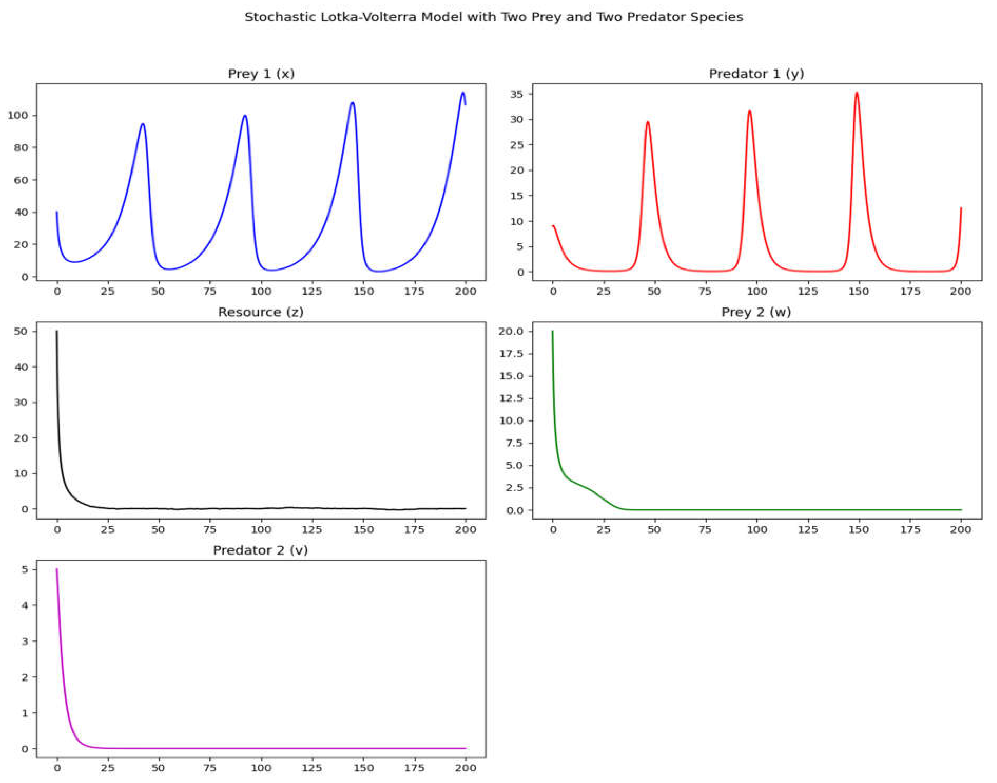
Figure 1. Note each variable separately oscillating with time.

This graph (graph 1.) with time on the x-axis and population size on the y-axis shows how the populations of prey and predators change over time according to the Lotka-Volterra model. You should see oscillations that represent the cycles of growth and decline in the predator and prey populations.

The plot typically shows cyclical behavior where the prey population increases, followed by an increase in the predator population. As the predators thrive, they reduce the prey population, which in turn causes the predator population to decline, and the cycle repeats.

We can extend the classic Lotka-Volterra predator-prey model to include a third equation that might represent another species or a factor such as a resource limitation affecting the prey population.

To extend the model to include an additional prey and predator species, we need to augment the system with two more differential equations, one for the second prey population, w, and one for the second predator population, v. Let’s assume that the second prey competes with the first prey for the same resource z, and the second predator competes with the first predator for the same prey x, to keep the model relatively simple.

Here’s the augmented system of equations (graph 2), where ρ and σ are the interaction terms between the original and the new prey and predator populations, respectively:

dx/dt = αx - βxy - ϵxz – ρxw

(3)

dw/dt = α’w - β’wy - ϵ’wz - ρ’wx

(4)

dy/dt = δxy - γy – σyv

(5)

dv/dt = δ’xw - γ’v - σ’vy

(6)

dz/dt = ζz(1 - z/k) - ηxz - η’wz + stochastic term

(7)

In this model:

w is the second prey population.

v is the second predator population.

α’, β’, δ’, γ’, ϵ’, η’, ρ’, σ’ are the growth, predation, death, and competition rates for the second prey and predator.

k is the carrying capacity of the resource.

The stochastic term is as previously defined, affecting the resource availability due to climate.

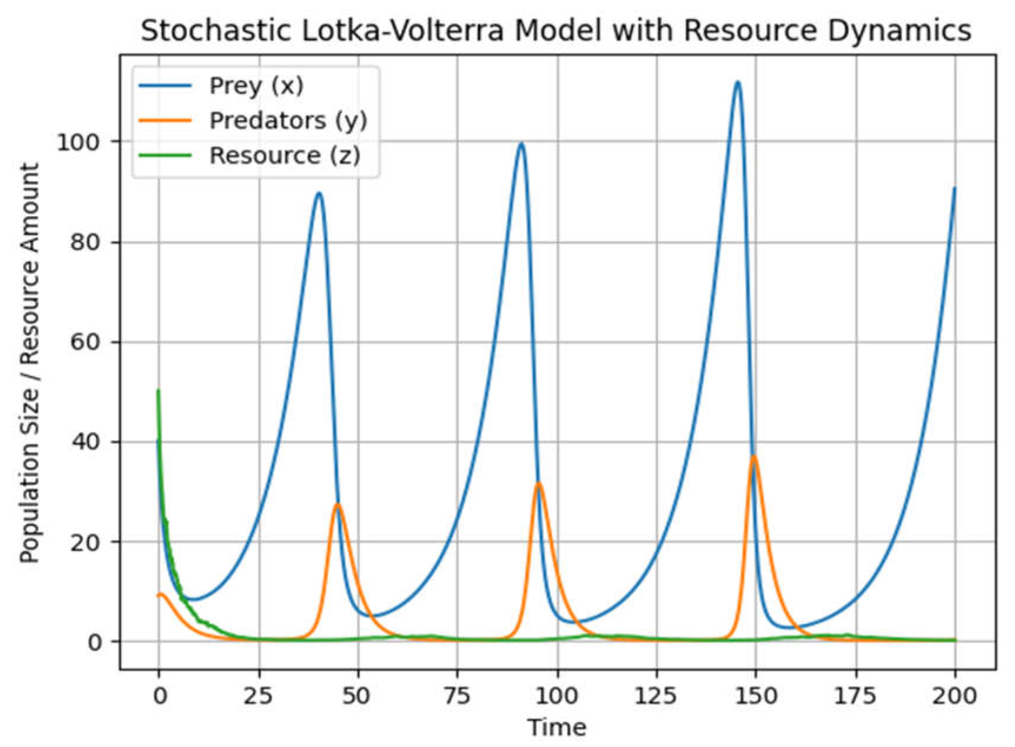
This graph (Graph2) adds a third differential equation to the system and solves for the dynamics over time. The graph produced will now show three lines, each representing the time evolution of the prey, predators, and the resource, respectively. The addition of the resource z introduces new dynamics to the model, where the availability of resources can limit the growth of the prey population, which in turn affects the predator population.

Remember that the specific behavior of the system will depend heavily on the chosen parameters and initial conditions, so the actual dynamics could vary significantly in different scenarios.

For simplicity, let’s modify the predator-prey-resource model by adding a stochastic term to the resource growth rate.

We use a simple implementation using an Euler-Maruyama approximation:

This model will produce a graph similar to the deterministic one, but the resource line will exhibit random fluctuations, representing the stochastic effects on the resource dynamics. Each run of this simulation will yield different results due to the random component.

Let’s say the climate factor, c(t), influences the resource regeneration rate, which could in turn impact the prey growth rate due to resource availability. To keep things simple, let’s consider climate as a periodic function (to model seasons) with added noise to represent random weather events.

In this modified model, the climate dynamics are represented by a sine function to model seasonal changes, plus a random noise term for unpredictability. The effective_zeta parameter in the resource differential equation is now influenced by this climate effect, which will cause the resource regeneration rate to oscillate with the seasons and fluctuate due to stochastic events.

The resulting graph (Graph 3) will show how the prey, predator, and resource populations are affected by the added climate dynamics. Due to the stochastic component, each simulation run can yield different outcomes, similar to real-world scenarios where weather and climate variability play significant roles in ecosystem dynamics.

The stochastic term is as previously defined, affecting the resource availability due to climate.

Here’s the augmented system of equations, where ρ and σ are the interaction terms between the original and the new prey and predator populations, respectively:

dx/dt = αx - βxy - ϵxz – ρxw

(7)

dw/dt = α’w - β’wy - ϵ’wz - ρ’wx

(8)

dy/dt = δxy - γy – σyv

(9)

dv/dt = δ’xw - γ’v - σ’vy

(10)

dz/dt = ζz(1 - z/k) - ηxz - η’wz + stochastic term

(11)

In this model:

w is the second prey population.

v is the second predator population.

α’, β’, δ’, γ’, ϵ’, η’, ρ’, σ’ are the growth, predation, death, and competition rates for the second prey and predator.

k is the carrying capacity of the resource.

The stochastic term is as previously defined, affecting the resource availability due to climate.

In this extended model, the new prey w and predator v are affected by and have an effect on the existing prey and predator populations through competition. The resource z is now also consumed by the new prey w, and its growth is limited by the carrying capacity k and influenced by stochastic climate effects.

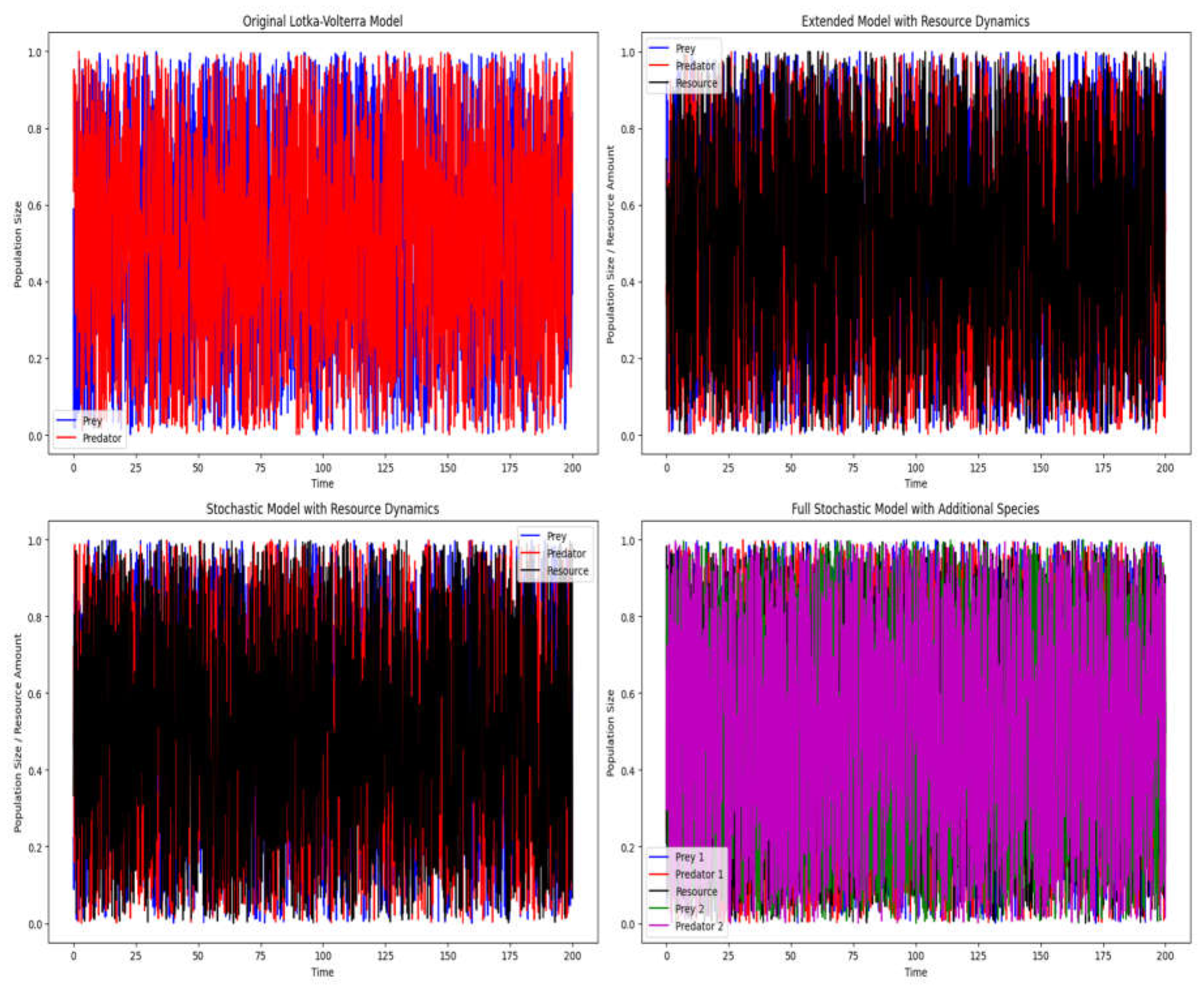
Here’s a hypothetical structure to organize the figures:

The original Lotka-Volterra model for a single prey-predator system.

The extended Lotka-Volterra model with resource dynamics.

The stochastic version of the extended Lotka-Volterra model with resource dynamics.

The further extended stochastic Lotka-Volterra model with two prey and two predator species.

Figure 3. Finally, the 4 graphs illustrate a simple model of crescent complexity and carriage of information.

3. Discussion

Understanding the central nervous system (CNS) is no easy feat—it’s a complex network made up of billions of neurons working together in a dynamic dance (just see Figure 2). According to Bear, Connors, and Paradiso (2001), these interactions within the CNS, and between the CNS and the environment, can be described using differential equations. These equations help us grasp processes like electrical and chemical signaling, synaptic plasticity, neural adaptation, and sensory processing—key areas in computational neuroscience.

At the individual neuron level, models like the Hodgkin-Huxley model use differential equations to describe how a neuron’s membrane potential changes in response to various inputs. This model captures the intricate behavior of neurons, as originally detailed by Hodgkin and Huxley in 1952. When looking at larger neuronal networks, we often represent them as systems of coupled differential equations, which take into account the connections between neurons and how these connections change over time, as discussed by Tsodyks and Markram in 1997.

Despite the power of these models, fully capturing the complexity of the CNS is a daunting task. The system’s nonlinearity, plastic nature, and the interactions between multiple scales—from molecular to cellular to whole systems—make it a challenging area of study (Koch & Segev, 1998; Felleman & Van Essen, 1991). Our current models, while helpful, are simplifications of the true biological processes (Churchland & Sejnowski, 1992).

Moreover, even with today’s advanced computational resources, simulating the entire CNS is still beyond our reach (Braitenberg & Schüz, 1991). To make progress, neuroscience often uses focused models that simplify specific parts of the CNS. This approach allows researchers to dive deeper into particular aspects, gradually building a more comprehensive understanding over time (Sporns, Tononi, & Kötter, 2005). As our computational methods and biological insights improve, these models will continue to evolve, reflecting our growing knowledge of the CNS and its interactions with the body and the environment (LeCun, Bengio, & Hinton, 2015).

The interwoven nature of emotions and reasoning, especially within the context of evolution, is a fascinating and intricate subject. Damasio (1994) highlights the deep connection between emotion, reason, and the human brain, emphasizing how our feelings play a crucial role in rational decision-making. This idea is echoed by Edelman (1989), who suggests that our conscious experiences are rooted in the physical workings of the brain.

From a structural viewpoint, the brain’s distributed hierarchical processing, described by Felleman and Van Essen (1991), underscores its complexity, enabling both emotional and cognitive functions. This complexity is further explored by Braitenberg and Schüz (1991), who provide geometric and statistical insights into cortical connections, helping us understand the anatomical basis for emotion and reasoning.

Advances in neural modeling, such as those introduced by Koch and Segev (1998), offer deeper insights into how neurons compute and contribute to higher-order functions. These models have been refined by researchers like Dayan and Abbott (2001), who delve into the theoretical aspects of neural function and behavior.

Emotions play a vital role in social bonding and survival, a concept that resonates with the work of Bear et al. (2001). They explore how the brain’s neurobiological mechanisms give rise to behavior and cognitive functions. Similarly, the research by Tsodyks and Markram (1997) on synaptic transmission and its role in memory and learning sheds light on the neural basis for the interaction between emotion and reasoning.

Sleep, as proposed by Sejnowski and Destexhe (2000), is crucial for cognitive processing and memory consolidation, which in turn influences the interplay between emotional and cognitive processes. This perspective on sleep enriches our understanding of how different states of consciousness affect the functionality of emotions and reasoning.

Moreover, viewing the brain as a computational entity, as described by Churchland and Sejnowski (1992), provides a framework for understanding how it processes both emotional and rational content. This computational approach is essential in unraveling the complex relationship between emotion and reasoning within the evolutionary landscape.

4. Conclusion

The complexity increases with each variable or equation added and the level of information transmitted also increases exponentially. Note, however, that this is a very simplistic model, but, one that can help to visualize the complexity of brain computation if we add millions of differential equations to the system, including ones that inhibit others as viewed by the adapted Lotka-Volterra Model. Despite the enormity of the task, one should not underestimate computational capacity, including recent artificial intelligence evolvements that will certainly accelerate exponentially computation load and performance.

Conflicts of Interest

The author declares no conflicts of interests

References

Hodgkin, A.L., & Huxley, A.F. (1952). A quantitative description of membrane current and its application to conduction and excitation in nerve. Journal of Physiology, 117(4), 500-544.
Hebb, D. O. (1949). The organization of behavior; a neuropsychological theory. Wiley.
Hubel, D. H., & Wiesel, T. N. (1962). Receptive fields, binocular interaction and functional architecture in the cat’s visual cortex. Journal of Physiology, 160(1), 106-154.
Felleman, D. J., & Van Essen, D. C. (1991). Distributed hierarchical processing in the primate cerebral cortex. Cerebral Cortex, 1(1), 1-47.
Braitenberg, V., & Schüz, A. (1991). Anatomy of the Cortex: Statistics and Geometry. Springer-Verlag.
Bear, M. F., Connors, B. W., & Paradiso, M. A. (2001). Neuroscience: Exploring the Brain. Lippincott Williams & Wilkins.
Kandel, E. R., Schwartz, J. H., & Jessell, T. M. (2000). Principles of Neural Science. McGraw-Hill.
Koch, C., & Segev, I. (Eds.). (1998). Methods in Neuronal Modeling: From Ions to Networks. MIT Press.
Sporns, O., Tononi, G., & Kötter, R. (2005). The human connectome: A structural description of the human brain. PLoS Computational Biology, 1(4), e42.
Dayan, P., & Abbott, L. F. (2001). Theoretical Neuroscience. MIT Press.
Mountcastle, V. B. (1997). The columnar organization of the neocortex. Brain, 120(4), 701-722.
Llinás, R. R. (2001). I of the Vortex: From Neurons to Self. MIT Press.
Dehaene, S. (2009). Reading in the Brain: The New Science of How We Read. Viking.
Damasio, A. (1994). Descartes’ Error: Emotion, Reason, and the Human Brain. Putnam Publishing.
Edelman, G. M. (1989). The Remembered Present: A Biological Theory of Consciousness. Basic Books.
Freeman, W. J. (2000). How Brains Make Up Their Minds. Columbia University Press.
Thagard, P. (2005). Mind: Introduction to Cognitive Science. MIT Press.
Sejnowski, T. J., & Destexhe, A. (2000). Why do we sleep? Brain Research, 886(1-2), 208-223.
Squire, L. R., et al. (2012). Fundamental Neuroscience. Academic Press.
Gazzaniga, M. S., Ivry, R. B., & Mangun, G. R. (2009). Cognitive Neuroscience: The Biology of the Mind. W. W. Norton & Company.
Tsodyks, M., & Markram, H. (1997). The neural code between neocortical pyramidal neurons depends on neurotransmitter release probability. Proceedings of the National Academy of Sciences, 94(2), 719-723.
Hinton, G. E., Osindero, S., & Teh, Y. W. (2006). A fast learning algorithm for deep belief nets. Neural Computation, 18(7), 1527-1554.
Raichle, M. E. (2006). Neuroscience. The brain’s dark energy. Science, 314(5803), 1249-1250.
LeCun, Y., Bengio, Y., & Hinton, G. (2015). Deep learning. Nature, 521(7553), 436-444.
Buzsáki, G. (2006). Rhythms of the Brain. Oxford University Press.
Penfield, W., & Boldrey, E. (1937). Somatic motor and sensory representation in the cerebral cortex of man as studied by electrical stimulation. Brain, 60(4), 389-443.
Tononi, G., Boly, M., Massimini, M., & Koch, C. (2016). Integrated information theory: from consciousness to its physical substrate. Nature Reviews Neuroscience, 17(7), 450-461.
Churchland, P. S., & Sejnowski, T. J. (1992). The Computational Brain. MIT Press.
Singer, W. (1999). Neuronal synchrony: a versatile code for the definition of relations? Neuron, 24(1), 49-65, 111-125.
Markram, H., et al. (2015). Reconstruction and Simulation of Neocortical Microcircuitry. Cell, 163(2), 456-492.

Figure 2. Variables put together in the same graph to better visualize increasing complexity. Next figure will show drastically increasing complexity and carriage of information.

Disclaimer/Publisher’s Note: The statements, opinions and data contained in all publications are solely those of the individual author(s) and contributor(s) and not of MDPI and/or the editor(s). MDPI and/or the editor(s) disclaim responsibility for any injury to people or property resulting from any ideas, methods, instructions or products referred to in the content.

© 2024 by the authors. Licensee MDPI, Basel, Switzerland. This article is an open access article distributed under the terms and conditions of the Creative Commons Attribution (CC BY) license (http://creativecommons.org/licenses/by/4.0/).

Copyright: This open access article is published under a Creative Commons CC BY 4.0 license, which permit the free download, distribution, and reuse, provided that the author and preprint are cited in any reuse.