1. Introduction
When solving many applied problems, there is often a need to minimize certain functional. Recently, a variety of minimization software packages have become available to scientists, providing access to highly-optimized minimization functions. For example, in one of the most popular libraries among the scientific community, SciPy [
1] of the Python programming language, multiparameter minimization functions are available, which can be divided into two classes: local minimization functions and global minimization functions. Local minimization functions include those that implement: the Nelder-Mead algorithm [
2], the modified Powell algorithm [
3], the conjugate gradient algorithm [
4], the Broyden-Fletcher-Goldfarb-Shanno (BFGS) algorithm [
5,
6,
7,
8], the Newton conjugate gradient algorithm [
9], the limited memory Broyden-Fletcher-Goldfarb-Shanno (L-BFGS-B) algorithm with box constraints [
10], a truncated Newton (TNC) algorithm [
11], the Constrained Optimization BY Linear Approximation (COBYLA) algorithm [
12], Sequential Least Squares Programming (SLSQP) [
13], a trust-region algorithm for constrained optimization [
14,
15], the dog-leg trust-region algorithm [
16], the Newton conjugate gradient trust-region algorithm [
17], the Newton Generalized Lanczos Trust Region (GLTR) algorithm [
18,
19], a nearly exact trust-region algorithm [
20]. Global minimization functions include those that implement: the Basin-hopping algorithm [
21], the “brute force” method [
22], the differential evolution method [
23], simplicial homology global optimization [
24], dual annealing optimization [
25], the DIRECT (Dividing RECTangles) algorithm [
26,
27].
The availability of such minimization software packages has significantly increased the efficiency of scientific work, since it has allowed scientific groups that do not specialize in numerical minimization methods not to waste time on software implementation of the minimization algorithms necessary in scientific work. However, it should be noted that the most popular minimization packages involve sequential calculations. This leads to the following problem: the computational complexity of many modern application problems requires such large amounts of calculations that these calculations cannot be performed on personal computers in a reasonable time.
This problem could be solved as follows. With the development of computing capabilities, the use of parallel computing and parallel programming technologies has become widespread, which make it possible to solve computationally complex problems in a reasonable time. The problem of long calculation is solved by parallelizing calculations between different computing nodes of a computer system. However, the fact that many popular minimization packages do not involve parallelization of calculations leads scientists to the following dilemma: either agree to an extremely long calculation, or try to implement minimization algorithms themselves and then parallelize them. In both cases, the time required to solve the scientific problem being solved may increase significantly.
It should be noted that many minimization software packages have recently begun to add parallel computing to their implementation on computer systems with shared memory. In practice, such systems are usually a computer with a single multi-core processor. As a result, within one computing node (for example, a personal computer), the running time of the algorithm can be reduced, but the maximum possible acceleration of the program is still limited by the capabilities of this computing node. Therefore, it is still relevant to develop software implementations that have the ability to use computing systems with distributed memory.
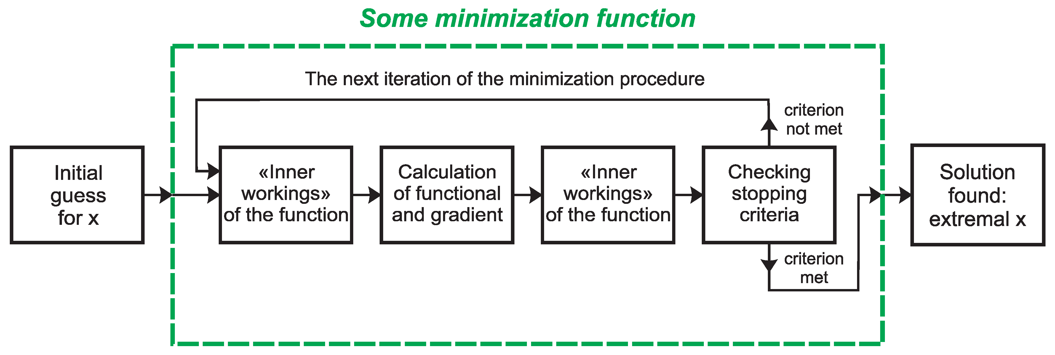
In connection with the above, a question arose: is it possible to parallelize the calculations that arise when using standard minimization functions, bypassing a detailed study of the computational algorithms that are implemented inside these functions? That is, is it possible to use the available minimization functions “as is”? Research has shown that this can be done. The structure of any minimization function is such (see
Figure 1) that the main calculations involve calculating the functional and, possibly, its gradient (in the case of using first-order minimization methods). And it is the functions that implement functional/gradient calculations that scientists implement independently in any case. As a consequence, only these calculations can be parallelized. This work is devoted to how this can be done relatively simply.
The structure of this work is as follows.
Section 2 describes the structure of the proposed parallel algorithm, formalizes the pseudo-code of this algorithm, and also describes the structure of the corresponding Python code that implements this algorithm using the mpi4py package. The mpi4py package for organizing the communication of various computing processes allows the use of MPI message passing technology, which is currently the main programming tool in parallel computing on systems with distributed memory. For convenience, the Python code is presented in the form of pseudocode that does not contain operations and function arguments that are unimportant for the perception of the algorithm.
Section 3 describes the full version of the software implementation of the parallel algorithm, which also uses the latest version of the MPI standard — MPI-4 [
28,
29].
Section 4 presents the results of test calculations demonstrating the strong scalability properties of the proposed software implementation.
Section 5 discusses possible ways to modify the proposed algorithm, taking into account the most frequently encountered situations in practice.
2. Parallel Algorithm
According to
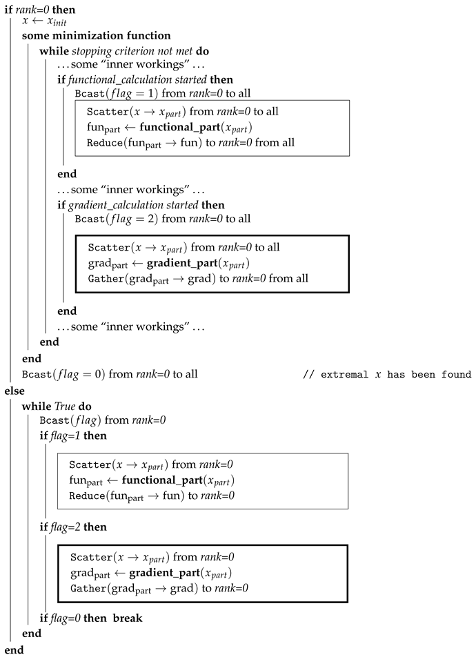
Figure 1, any minimization function, when executed, repeatedly calls functions that are specified by the user and implement the calculation of the functional and its gradient. Given that the minimization function used is sequential, it will only be called by the master process. Therefore, functions that are specified by the user and implement the calculation of the functional and its gradient will be split into two pairs of functions: 1) functions that are called by the master process only within the minimization function, and 2) auxiliary functions that are called by all processes.
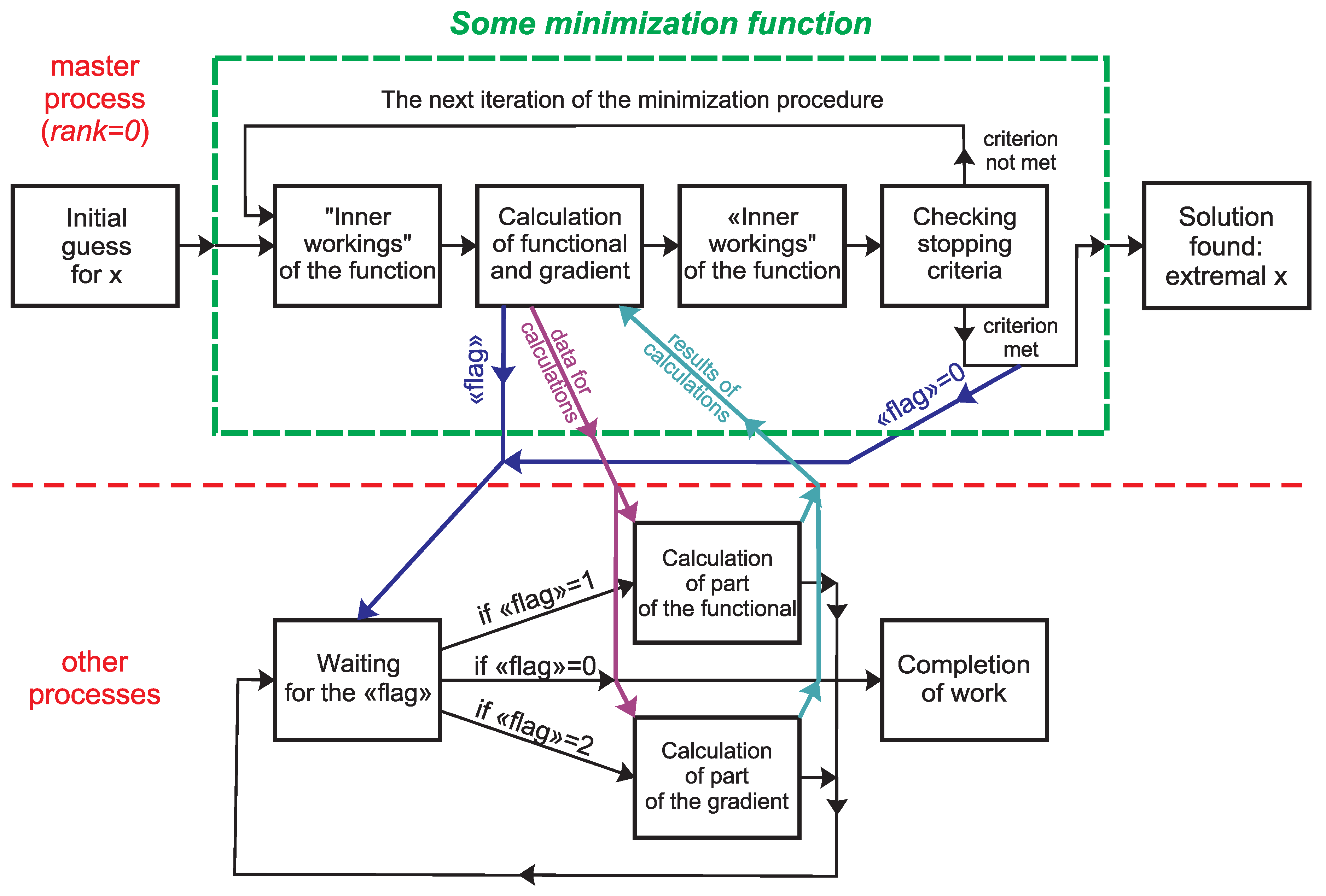
Functions that are called only by the master process must first implement the distribution of a “flag” to all other processes, based on which the remaining processes can conclude what needs to be done next: 1) calculate their part of the functional, or 2) calculate their part of the gradient. The data needed for calculations is then distributed across all processes. After this, the master process launches an auxiliary function, through which part of the functional or part of its gradient is calculated, for which the master process is responsible for calculating. Then, data from intermediate calculations performed in parallel is collected from all processes, and the final result of calculating the functional and its gradient is aggregated.
After the minimization function completes its work on the master process, the master process sends a “flag” to all other processes, based on the value of which the other processes can conclude that it is necessary to stop working.
The other processes run an endless “while” loop, inside which each process waits to receive a “flag”, based on the value of which it concludes what needs to be done next: 1) calculate its part of the functional, 2) calculate its part of the gradient, 3) finish the job. Further, in the case of the first two options, data for calculations is expected and after receiving it, an auxiliary function is launched, through which the calculation of its part of the functional or its gradient is implemented. Next, the results obtained are sent to the master process.
This algorithm is illustrated in
Figure 2 and formalized in the form of the following pseudocode (see algorithm 1), in which the master process has
rank = 0.
|
Algorithm 1:Pseudocode of a universal parallel algorithm. Frames highlight pairs of blocks that are executed in parallel. Distribution of data from MPI master process with rank=0 to other MPI processes is carried out using the MPI routine of collective communication of processes Scatter(), but depending on the features of the minimized functional, the distributing data can be implemented with using one of the MPI routines Bcast(), Scatterv(), Reduce_scatter(), etc. |
 |
The Python code that implements this algorithm will be quite compact. Its structure in the form of Python pseudocode is presented below. At the same time, for clarity: 1) some of the arguments of the functions used are omitted, 2) the syntax is simplified.
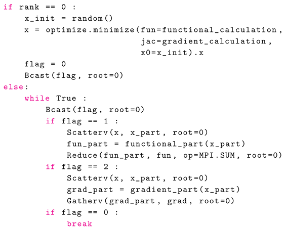
Here the functions functional_calculation() and gradient_calculation(), which are called by the master process inside the minimization function optimize.minimize() from the SciPy package, have the following structure:
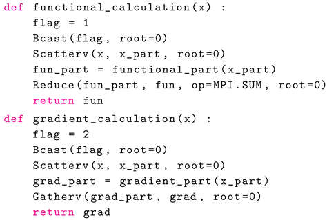
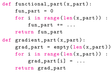
and the auxiliary functions
functional_part() and
gradient_part(), which are called by all processes, have the following general form:

Note. Here it is assumed that in order to calculate its part of the functional or its gradient, each MPI process must know not all the components of the next approximation for the vector x, which is contained in the array x, but only part of its components , which are contained in the array x_part. Situations are quite common when each MPI process must know all the components of the next approximation for the vector x. In this case, you may need to use the MPI routine Bcast() instead of the MPI routine Scatter(v)().
3. Description of the Full Version of the Software Implementation of the Parallel Algorithm (Using the MPI-4 Standard)
Next, we will describe the complete Python code that implements the algorithm 1. But first, the following remark must be made. The software implementation structure proposed in the previous section contains collective communications between processes with the same argument list which are repeatedly executed within the inner loop of a parallel computation. In such a situation, it may be possible to optimize the communications by binding the list of communication arguments to a persistent communication request once and, then, repeatedly using the request to initiate and complete messages. The peculiarity of the MPI-4 standard (2021) is that it introduced MPI routines that allow this to be done for operations of collective communications of processes.
For example, the result of running the MPI routine Bcast() is equivalent to the sequence of launching the MPI routines Bcast_init() “+” Start() “+” Wait(). Moreover, if the MPI routine Bcast_init() is launched multiple times with the same set of arguments, the result of calling Bcast_init() will be the same. This makes it possible to move this action “out of brackets”, that is, out of the loop through which it is called repeatedly.
That is, in order to use more advanced versions of the MPI routines for collective communication of processes from the MPI-4 standard, it is necessary to perform the following sequence of changes.
Before the main loop while, it is necessary to generate persistent communication requests using MPI routines of the form request[] = Bcast_init() for all routines of collective communications of processes Bcast(), Scatterv(), Reduce() and Gatherv(), which are called multiple times with the same set of arguments.
Replace MPI routine calls with a sequence of function calls Start(request[]) “+” Wait(request[]).
So, taking into account the comments made, the parallel software implementation of the algorithm 1 will take the following form (in this case, the program code will be commented block by block, but all blocks with numbered lines will form a single program code).

Lines 1–3 import the necessary functions. When importing MPI (line 1), the MPI part of the program is initialized. Based on the results of lines 5-7, each MPI process, on which this program code is executed, knows 1) the total number numprocs of processes participating in the calculations, and 2) its identifier rank in the communicator comm, which contains all the processes on which the program runs.


In line 8, the number of components of the model vector
x is determined, and then in lines 11–15, on the master process with
rank = 0, auxiliary arrays
counts and
displs, necessary for MPI routines
Scatterv() and
Gatherv() (which will be used to distribute components of the vector
x among processes or to collect intermediate calculation data from all processes), are prepared. Thus, the array
counts contains information about the number of elements sending to each process (or received from each process). Those, array element
counts[k] contains the value
— number of components of part
of vector
x, for which MPI process with
rank = k is responsible for processing. The algorithm for determining the elements of
counts is such that the maximum difference between any two elements of this array is 1, but the sum of all elements of this array is equal to
N:
It should be noted that the values of the array elements counts and displs will be needed further only on the process with rank = 0 (master process). These values will not be used by other processes. But taking into account the fact that the arrays counts and displs will be arguments to the functions Scatterv() and Gatherv(), which are called on all processes, then the corresponding Python objects formally must be initialized. This is done on line 17 for processes with rank >= 1.
Line 19 allocates memory space for the array N_part, which will contain only one value — the number of elements of the vector part , for which the MPI process, on which this program code is running, is responsible. It is necessary to recall that formally this number must be a numpy-array, since the MPI routines used only work with numpy-arrays. In line 20, using the MPI routine Scatter(), this array is filled with the corresponding value from the array counts, contained only in the process with rank = 0. Now the MPI process with ramk = k knows its value , contained on this MPI process in the array N_part.
Next, an array x_model is formed, which contains the values of the model vector , with which the solution to the minimization problem will be compared.

In lines 21–24 this array is formed only on the master process with rank = 0 (line 22), and then in lines 27–28, using the MPI routine Scatterv(), it is distributed in parts from the process with rank = 0 across all processes where the corresponding parts are stored in the array x_model_part. To do this, in line 26, memory space is preliminarily allocated for these arrays.
Now begins the consideration of the main part of the program, which directly implements the algorithm considered in the work.
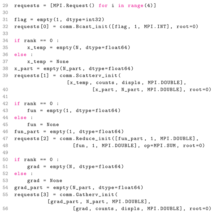
First, it is necessary to generate persistent communication requests for all MPI routines of collective communications of processes that will be called repeatedly.

Line 29 creates the array requests, which will contain the values of the returned parameters, which, in turn, will be used to identify specific persistent communication requests for collective communications. Next, persistent communication requests are generated for the MPI routines Bcast() (lines 31–32), Scatterv() (lines 34–40), Reduce() (lines 42 —48), Gatherv() (lines 50–56).
The generation of such persistent communication requests for collective communications is the same, so it will be explained only using the example of the formation of a persistent communication request for collective communication for the MPI routine Scatterv() (lines 34–40). Line 35 allocates memory space for the array x_temp only on the process with rank = 0 (this array will contain the values of the vector x, but the meaning of the postfix _temp will be explained later when filling this array with specific values). Its contents will not be used by other processes. But taking into account the fact that the array x_temp is an argument of the MPI routines Scatterv_init() (lines 39–40), which are called on all processes, the corresponding Python object must formally be initialized. This is done on line 37 for processes with rank >= 1. Line 38 allocates memory space for the array x_part.
It is necessary to note the following important point in the formation of persistent communication requests. The arguments of the corresponding functions are numpy-arrays (for example, in the case considered, the arrays x_temp and x_part), namely fixed memory areas associated with these arrays. When initializing generated communication requests using the MPI routine MPI.Prequest.Start(), all data will be taken/written to these memory areas, which are fixed once when the corresponding persistent communication request is generated. Therefore, it is necessary to first allocate space in memory for all arrays that are arguments to these functions; and during subsequent calculations, ensure that the corresponding calculation results are stored in the correct memory areas.
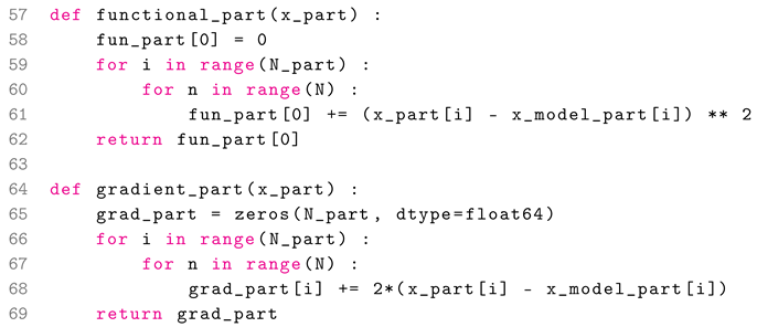
Next, the auxiliary functions functional_part() and gradient_part() are defined, which are called by all processes.

These auxiliary functions contain calculations of the functional, which for simplicity is given as
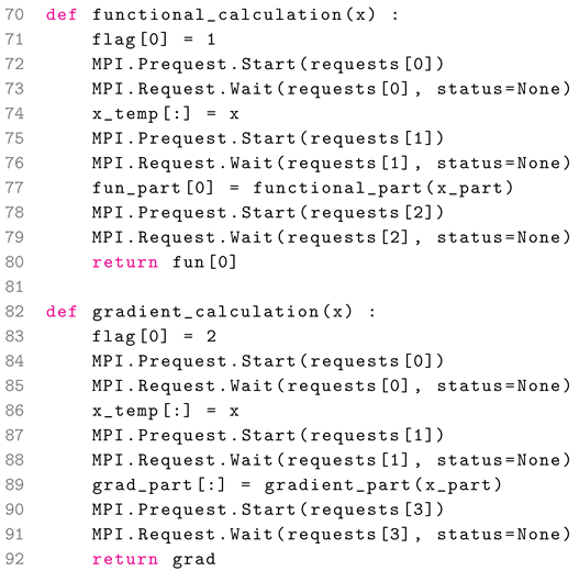
Next, the functions functional_calculation() and gradient_calculation() are defined, which are called by the master process with rank = 0 inside the minimization function optimize.minimize() from the SciPy package.

The structure of these functions fully corresponds to the structure proposed at the end of the previous section (
Section 2). Therefore, it is necessary to note only the features of their software implementation. This will be done using the function
functional_calculation() as an example.
In lines 72–73, the functionality of the MPI routine Bcast() is executed, the persistent communication request for which was generated in line 32. Since the corresponding MPI routine is non-blocking, we must wait until the end of its execution (line 73).
In lines 75–76, the functionality of the MPI routine Scatterv() is executed, the persistent communication request for which was generated in lines 39–40. Since the corresponding MPI routine is non-blocking, we must wait for its execution to complete (line 76).
In this case, it is necessary to note the role of the array x_temp (line 74). This array will contain the values of the vector x, which could not be redefined, but directly distributed between other processes. But due to the fact that it is often unknown how the minimization function is structured internally, which at each iteration redefines the vector x, it may turn out that a new place in memory is allocated for the next approximation of this vector at this iteration. Therefore, for the purpose of insurance, the values of this array are copied to a pre-allocated fixed location in memory (line 35) in order for the function Scatterv(), generated by a persistent communication request, to work correctly.
In lines 78–79, the functionality of the MPI routine Reduce() is executed, the persistent communication request for which was generated in lines 47–48. Since the corresponding MPI routine is non-blocking, we must wait for its execution to complete (line 79).
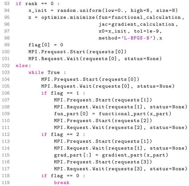
The following is the Python code that implements the main part of the algorithm 1.

The structure of this code fully corresponds to the structure proposed at the end of the previous section (
Section 2). Therefore, it is necessary to note only the features of its software implementation.
In lines 100–101 and 104–105, the functionality of the MPI routine Bcast() is executed, the persistent communication request for which was generated in line 32.
In lines 107–108 and 113–114, the functionality of the MPI routineScatterv() is executed, the persistent communication request for which was generated in lines 39–40.
In lines 110–111, the functionality of the MPI routine Reduce() is executed, the persistent communication request for which was generated in lines 47–48.
In lines 116–117, the functionality of the MPI routine Gatherv() is executed, the persistent communication request for which was generated in lines 55–56.
4. Efficiency and Scalability of Software Implementation of the Proposed Parallel Algorithm
To test the efficiency and scalability of the proposed software implementation of the parallel algorithm, the computing section “test” of the supercomputer “Lomonosov-2” [
30] of the Research Computing Center of Lomonosow Moscow State University was used. Each computing node in the “test” section contains a 14-core Intel Xeon E5-2697 v3 2.60GHz processor with 64 GB of RAM (4.5 GB per core) and a Tesla K40s video card with 11.56 GB of video memory (not used in calculations).
Remark. The program described in
Section 3 was tested. However, in addition to the file “example_MPI-4.py”, which contains this program, the digital version of the article also contains the file “example_MPI-3.py”, which contains a simplified version of the program that uses only MPI routines from the MPI-3 standard.
The parallel version of the program was launched with each MPI process bound to exactly one core. The software packages used were 1) mpi4py version 4.0.0.dev0, 2) numpy version 1.26.4, 2) scipy version 1.12.0, 4) mpich version 4.1. 1.
The scheme of numerical experiments repeats the scheme described in the work [
31]. The program was launched on a number of processes
numprocs, for which the running time
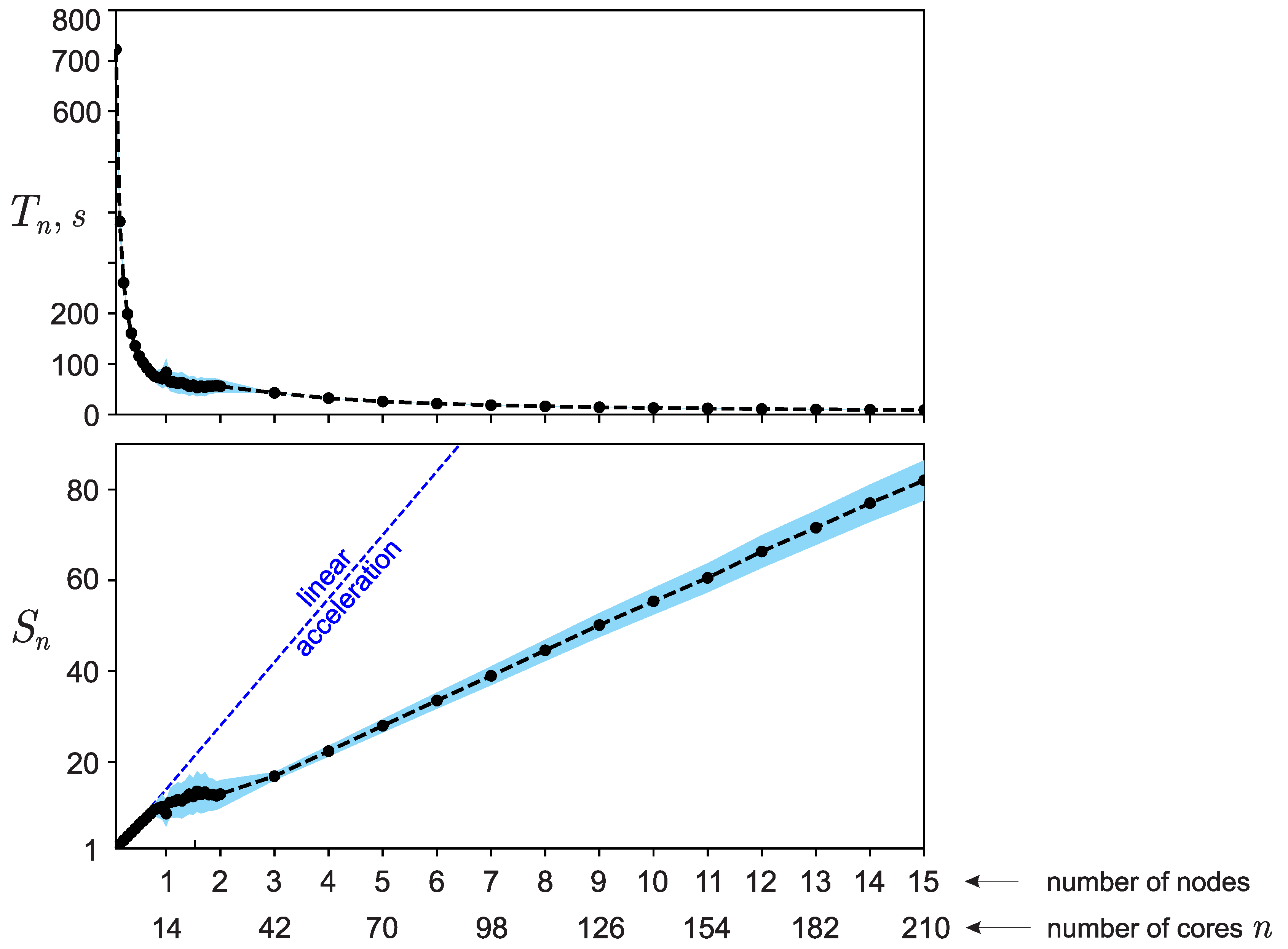
of the computational part of the program was recorded (see
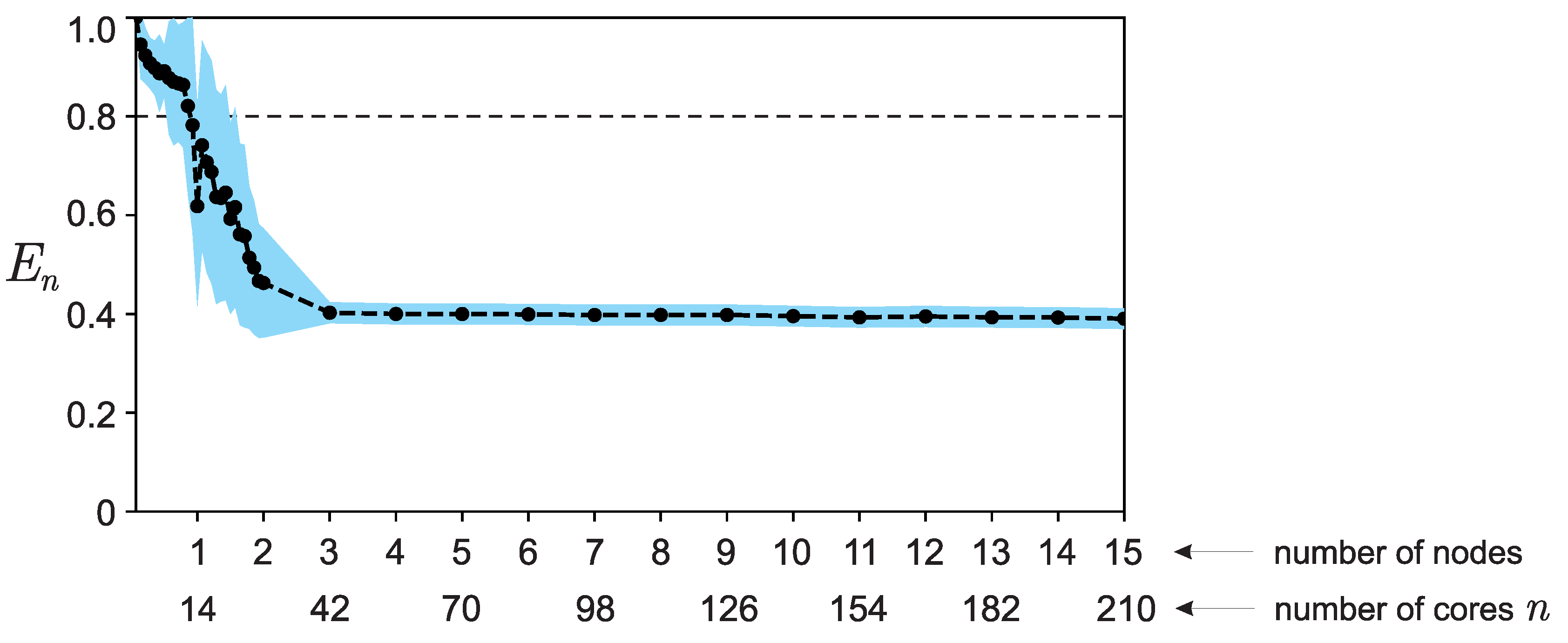
Figure 3). Using the estimated running time
of the sequential version of the algorithm, the speedup
was calculated using the formula
(see
Figure 3), and then efficiency
of software implementation (see
Figure 4).
The calculations were carried out for the parameter
(number of components in the model vector
x), for which the running time of the computational part of the serial version of the program was ∼ 752 seconds. The results shown in
Figure 3 and
Figure 4 correspond to the averaged values over a series of runs (100 runs for each value
n). At the same time, the graphs also show a corridor of errors
and
.
Errors for the obtained average values of acceleration and efficiency were calculated using the error formula for indirect measurements. In general, such a formula for the quantity
N, depending on direct measurements
,
, with known standard deviations
, has the form
Thus, for the acceleration calculated by the formula
the errors are calculated as
where
— estimate of the standard deviation for each measurement
.
For efficiency calculated using the formula
, the errors are calculated as
As can be seen from
Figure 4 the efficiency decreases in the interval from
to
and then remains constant. Formally, one could say that from this figure it can be concluded that the parallel software implementation of the algorithm, within certain limits, has good efficiency and good strong scalability over most of the range of the number of cores used for calculations. However, the indicated period of change in efficiency raises questions. Such a result would be easy to explain only in the case of a sharp deterioration in efficiency, starting from
. When
, only one node is used for calculations, as a result of which there is practically no overhead for the interaction of computing nodes (message transmission over the network is not used). Starting from
, 2 nodes already take part in the calculations, as a result of which the communication network is involved and significant overhead may appear for receiving/transmitting messages between computing nodes. Moreover, with an increase in the number of computing nodes used, the share of costs for receiving/transmitting messages should only increase.
The study of this issue revealed the following feature of the computing equipment used for test calculations. With the current settings of the installed packages and the “Lomonosov-2” supercomputer, when running programs using the mpirun utility from the mpich package, about 0-4 cores appear on each computing node, operating on average 2.28 times slower than the rest. The operating time of the entire parallel program is determined by the operating time of the slowest process, and as the number of computing processes n increases (each of which is executed on its own core of a multi-core processor), the probability of using “slow” cores increases, which is why the efficiency decreases relatively smoothly on the first two computing nodes, and then stops at the value (i.e., starting from three computing nodes, with a probability close to one, ”slow” cores begin to be used).
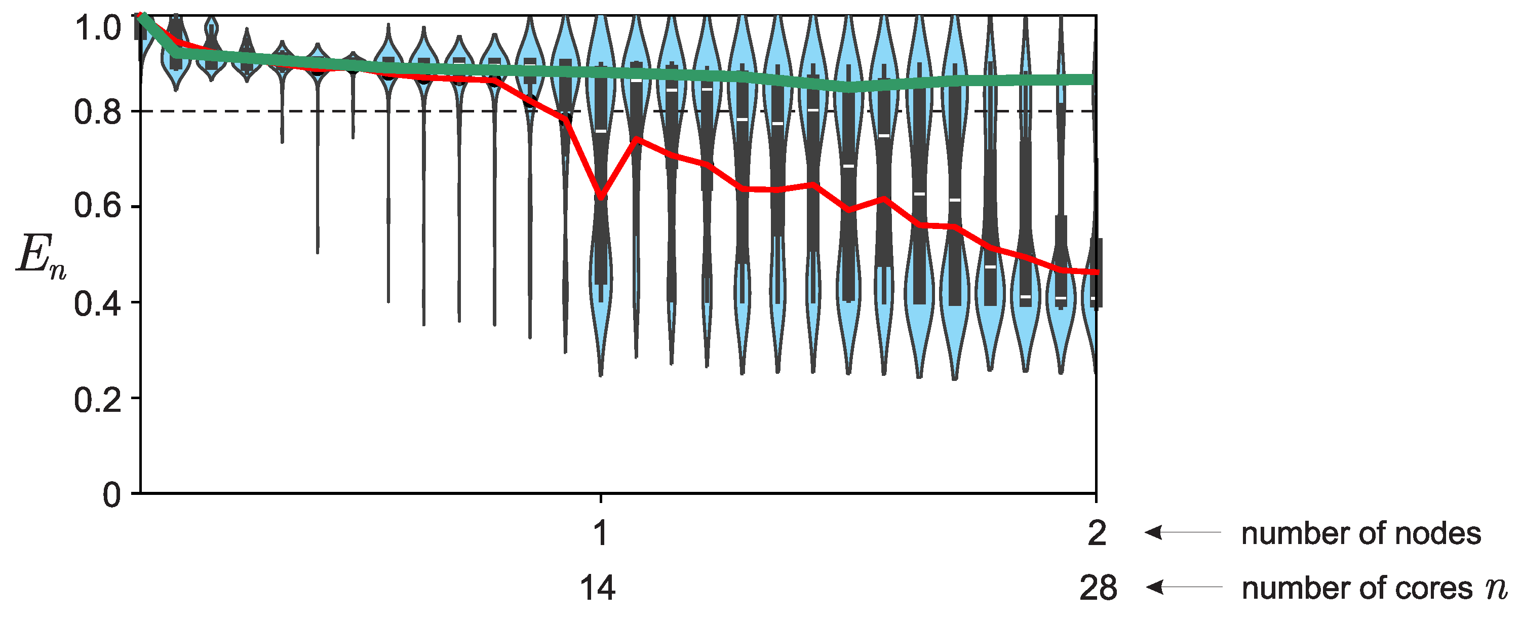
For values of the number of cores
, a graph was constructed showing the distribution of efficiency values over a series of runs for each value of
n (100 runs for each value). The resulting distributions (see
Figure 5) are not normal, since they contain two pronounced peaks: in the presence and absence of “slow” cores. Therefore, using the average of these values (see
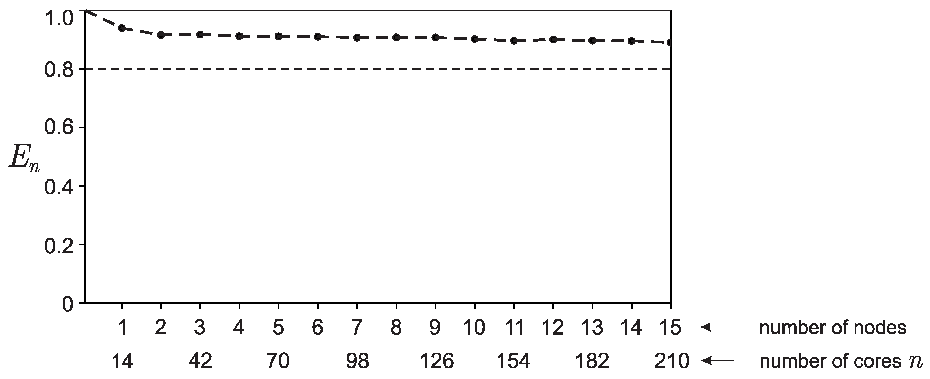
Figure 4) to characterize the properties of strong scalability of a software implementation of a parallel algorithm is not entirely correct — it is better to use values corresponding to the maximums of the distribution (see
Figure 6).


 and the auxiliary functions functional_part() and gradient_part(), which are called by all processes, have the following general form:
