Reliability Analysis of Distorted Distributions using Aging Intensity Function

Preprint

Article

Reliability Analysis of Distorted Distributions using Aging Intensity Function

Altmetrics

Downloads

102

Views

Comments

This version is not peer-reviewed

This preprints belongs to the Topic

Advanced Systems Engineering: Theory and Applications, 2nd Volume

Submitted:

08 June 2024

Posted:

10 June 2024

You are already at the latest version

Alerts

Abstract

This paper presents the preservation property of the average intensity order and the preservation property of the monotonic average intensity classes under distorted distributions. Several sufficient conditions are given to get the preservation properties. It is shown that the imposed conditions are achievable as we examine in some examples. The preservation of the average intensity order and the preservation of the decreasing average intensity class under the structure of a parallel system with independent and identically distributed components' lifetime are made. A lower bound for the average intensity function of a random lifetime with an increasing failure rate in average distribution is derived. The results are applied to some semiparametric models as a particular standard family of distorted distribution.

Keywords:

Subject: Computer Science and Mathematics - Probability and Statistics

MSC: 60E05, 60E15, 62N05

1. Introduction and Preliminaries

The notions of aging are very important because they reveal how the performance of an object having a random lifetime changes over time. The aging characteristics of a lifetime unit can be recognized by the distribution of the length of its lifetime. The aging aspect of a lifetime distribution is clearly different from the frequency aspect of this distribution, because it is not generally correct to say that a period in which failures are frequently observed is necessarily the time interval in which aging occurs more rapidly. The concept of aging is very useful for engineers in the context of reliability, for risk supervisors in the context of risk management and for experts in survival analysis. Due to design flaws, any technical system or component that is put into service will eventually cease to function as intended. Reliability theory states that the aging process, i.e. the gradual loss of a system or component’s total lifetime over time, is a representation of this physical reality. Different reliability measures that characterize the aging features of a life distribution have been developed in the literature (see, e.g., Barlow and Proschan [3], Lai and Xie [20], Marshall and Olkin [22]); these measures can also be used to define distinct stochastic ordering between the random variables that characterize the lifetimes of two units or objects. When comparing two life distributions with regard to various dependability metrics, these stochastic ordering can be helpful. The literature contains several examples of these stochastic orders. A comprehensive review of the several stochastic orders and dependability metrics may be found in the monographs written by Shaked and Shanthikumar [34], Li and Li [21] and Belzunce et al. [4].

In the literature, there are numerous reliability characteristics to measure aging phenomenon in lifetime units. Hazard rate function, mean residual lifetime function are very well-known among other various measures of aging. According to Jiang et al. ([14]), a system’s aging can be qualitatively represented by its hazard rate. In order to quantitatively assess the aging property of a system, the concept of aging intensity

(A I)

function has been introduced in the literature for evaluating the aging property of a unit (that may be a system or a living organism) quantitatively. The

A I

function of X which is denoted by

L_{X} (t)

created by Jiang et al. ([14]). This concept is defined as the ratio of the instantaneous hazard rate (h.r.)

h_{X} (t)

to the average hazard rate

H_{X} (t) = \frac{1}{t} \int_{0}^{t} h_{X} (τ) d τ

, which is given by

\begin{matrix} L_{X} (t) & : = \frac{h_{X} (t)}{H_{X} (t)} \\ = \frac{- t f (t)}{\bar{F} (t) ln (\bar{F} (t))}, t > 0, \end{matrix}

(1.1)

where f and

\bar{F}

are the probability density function (p.d.f.) and the survival function (s.f.) of the random variable (r.v.) X, respectively. In the context of reliability engineering, the

A I

function has been played a prominent role. Nanda et al. [26] derived some stochastic properties of various distributions in terms of the

A I

function. They defined a stochastic order called aging intensity order using the

A I

function and also proposed two monotonic aging classes of lifetime distributions based on the

A I

function. With regard to the

A I

function, Bhattacharjee et al. [5] investigated the behavior of some generalized Weibull models and certain system characteristics. Szymkowiak [35] presented some characterization results on Weibull- and inverse-Weibull-related distributions using the

A I

function. Using right-censored data, Misra and Bhattacharjee [24] examined the

A I

function and the hazard rate function in a case study of bone marrow transplant recipients with acute leukemia. Several aging classes were defined by Bhattacharjee et al. [6] using the harmonic, geometric and arithmetic averages of the

A I

function to determine their monotonicity. Giri et al. [10] derived the

A I

function of recent continuous Weibull distributions and obtained generalizations of a few recent Weibull models. Rasin et al. [31] proposed a novel nonparametric estimator of the

A I

function and established asymptotic behaviours of the derived estimator under suitable regularity conditions. Jiang et al. [15] and Jiang et al. [16] conducted the methods of parameter estimation on heavily censored data using the

A I

function. Raymarakkar Sidhiq et al. [32] proposed two nonparametric estimators for the

A I

function based on right-censored dependent data scheme and studied their properties.

The use of distorted distributions in reliability theory makes them very interesting (see, for instances, Navarro et al. [27], Navarro and del Águila [29] and Burkschat and Navarro [7]) and actuarial sciences (see Quiggin [30], Yaari [36] and Schmeidler [33]). The introduction of distorted distributions into actuarial science in recent decades has led to their application to a multitude of insurance-related issues, most notably the calculation of risk measures and insurance premiums (for further details see Goovaerts et al. [11] and the references therein). In the literature, there are some publications that link stochastic orderings and skewed distributions. A general survey on this topic can be found in Shaked and Shanthikumar [34]. To address applications of stochastic orders in actuarial science one may refer to Müller and Stoyan [25] and Denuit et al. [9]).

Let X and Y be two non-negative r.v.s which represent the lifetime of two items with aging intensity functions

L_{X}

and

L_{Y}

, respectively. Then, it is said that X is smaller than Y in the average intensity order (denoted as

X \leq_{A I} Y

) if

L_{X} (t) \geq L_{Y} (t),

for all

t \geq 0

. Nanda et al. [26] focused on the closure properties of the

A I

order under series systems with heterogenous component lifetime. They also remarked that the

A I

order is not closed under the formation of parallel system with independent and identically distributed (i.i.d.) component lifetimes. Nanda et al. [26] also revealed some preliminary properties of non-monotonic

A I

-based aging classes. In this direction, let X be a non-negative r.v. denoting the lifetime of an item. It is said then that X has increasing [decreasing] average intensity (

I A I

) [

D A I

] property whenever

L_{X} (t)

is a non-decreasing (non-increasing) function of

t \geq 0

. Let us consider a non-negative r.v. X with s.f.

\bar{F}

. Let

ν : [0, 1] \to [0, 1]

be a non-decreasing function such that

ν (0) = 0

and

ν (1) = 1

. The function

ν

is called a distortion function. We will suppose that

X_{ν}

is a non-negative random variable with s.f.

{\bar{F}}_{ν} (t) = ν (\bar{F} (t))

. The r.v.

X_{ν}

is said to have a distorted distribution. The purpose of the current study is to establish sufficient conditions for the preservation of the

A I

order and

I A I

and

D A I

classes under distorted distributions. To be more specific, we find conditions under which

X \leq_{A I} Y ⟹ X_{ν} \leq_{A I} Y_{ν},

and, further, we obtain conditions to get

X \in I A I (D A I) ⟹ X_{ν} \in I A I (D A I) .

It is seen that the lifetime of a parallel system with i.i.d. component lifetimes has a distorted distribution with

ν (u) = 1 - {(1 - u)}^{n}

. We show in examples that the results of the paper are satisfied for this specific distortion function. Therefore, under some mild conditions we indeed prove that a parallel system enjoys the closure property with respect to the

A I

order and also closure property with respect to the

D A I

class.

In what follows, some preliminaries which are essential to our development are given. Denote by X, the lifetime of a device which has c.d.f. F, s.f.

\bar{F}

and p.d.f. f (if it exists). Then, the h.r. function of X is defined as:

h_{X} (t) = lim_{δ \to 0^{+}} \frac{1}{δ} P (X \leq t + δ | X > t) = \frac{f (t)}{\bar{F} (t)}, t \geq 0 : F (t) < 1 .

The h.r. function which is uniquely determines the underlying distribution, measures the instantaneous risk for failure of an object at the age t.

The next definition is concerning stochastic comparison of random lifetimes according to their magnitude.

Definition 1.1.(Shaked and Shanthikumar [34]) Let X and Y denote two random lifetimes, such that X and Y have s.f.s

\bar{F}

and

\bar{G},

respectively. It is said that X is greater than (or equal to) Y in the usual stochastic order (denoted as

X \geq_{s t} Y

) whenever

\bar{F} (t) \geq \bar{G} (t),

for all

t \geq 0

The following definition presents an aging class of lifetime distributions.

Definition 1.2.(Lai and Xie [20]) It is said that X has increasing failure rate in average (

I F R A

) property, written as

X \in I F R A

, if

\frac{1}{t} \int_{0}^{t} h_{X} (x) d x

is increasing in

t > 0

The following key definition is adopted from Karlin [17].

Definition 1.3.

Let

l (x, y)

be a non-negative function. We say that f is totally positive of order 2 (or shortly, f is

T P_{2}

) in

(x, y) \in X \times Y

where

X

and

Y

are two arbitrary subsets of

R = (- \infty, + \infty)

when

\begin{matrix} f (x_{1}, y_{1}) & f (x_{1}, y_{2}) \\ f (x_{2}, y_{1}) & f (x_{2}, y_{2}) \end{matrix} \geq 0, f o r a l l x_{1} \leq x_{2} \in X, a n d f o r a l l y_{1} \leq y_{2} \in Y .

(1.2)

If the direction of the inequality given after determinant in (2.2) is reversed then f is said to be reverse regular of order 2 (f is

R R_{2}

) in

(x, y) \in X \times Y

The materials and the contents of the paper are organized subsequently as follows. In Section 2, the preservation property of the

A I

order under distorted distributions is established. In Section 3, we derive a lower bound for the

A I

function of a random lifetime possessing the

I F R A

properrty. In Section 4, the preservation property of the

I A I

and

D A I

classes under distorted distributions is studied. In Section 5, we apply our results on some families of semiparametric models. In Section 6, we gather some remarks and provide some explanations ion current research and also clarify some open problems for future research.

2. Preservation of the Average Intensity Order Under Distortion

In this section, the

A I

comparison between two base distributions is developed to the

A I

comparison of the corresponding distorted distribution. We will use the following technical lemmas to prove the main results.

Lemma 2.1.

Let

Φ (u) = \frac{u . ν^{'} (u)}{ν (u)}

. If

\frac{Φ (x^{α})}{Φ (x)}

is decreasing (increasing) in

x \in [0, 1]

for every

α \in [0, 1]

, then

K_{ν} (u) : = \frac{- ln (u) Φ (u)}{- ln (ν (u))}

is increasing (decreasing) in

u \in [0, 1]

Proof.

We prove the non-parenthetical part. The proof of other part is quite similar. By making the change of variable

y = - ln (u)

K_{ν} (u)

, one realizes that

K_{ν} (u)

is increasing in

u \in [0, 1]

if, and only if,

K_{ν} (e^{- y})

is decreasing in

y \geq 0

. One has

K_{ν} (e^{- y}) = \frac{y e^{- y} ν^{'} (e^{- y})}{- ν (e^{- y}) ln (ν (e^{- y}))}, f o r a l l y \geq 0 .

Note that, for all

y \geq 0,

- ln (ν (e^{- y})) = \int_{0}^{y} e^{- s} \frac{ν^{'} (e^{- s})}{ν (e^{- s})} d s = \int_{0}^{y} Φ (e^{- s}) d s .

(2.3)

Clearly,

K_{ν} (e^{- y})

is decreasing in

y \geq 0

if, and only if,

1 / K_{ν} (e^{- y})

is increasing in

y \geq 0

. By using Eq. (2.3), we get

\begin{matrix} \frac{1}{K_{ν} (e^{- y})} & = \frac{- ln (ν (e^{- y}))}{y e^{- y} \frac{ν^{'} (e^{- y})}{ν (e^{- y})}} \\ = \frac{1}{y} \int_{0}^{y} \frac{Φ (e^{- s})}{Φ (e^{- y})} d s \\ = \int_{0}^{1} \frac{Φ (e^{- α y})}{Φ (e^{- y})} d α . \end{matrix}

From assumption,

\frac{Φ (x^{α})}{Φ (x)}

is decreasing in

x \in [0, 1]

for every

α \in [0, 1]

, thus

\frac{Φ (e^{- α y})}{Φ (e^{- y})}

is increasing in

y \geq 0

. Thus,

1 / K_{ν} (e^{- y})

is increasing in

y \geq 0

□

The following lemma will be used in the sequel.

Lemma 2.2.

Let

α \in [0, 1] .

Then,

\frac{1 - x}{1 - x^{α}}

is increasing in

x \in (0, 1)

Proof.

Fix

α \in [0, 1] .

We show that

\frac{\partial}{\partial x} \frac{1 - x}{1 - x^{α}} \geq 0,

for all

x \in (0, 1)

. One gets

\frac{\partial}{\partial x} \frac{1 - x}{1 - x^{α}} \overset{s g n}{=} (1 - α) x^{α} + α x^{α - 1} - 1,

which is non-negative if, and only if,

(1 - α) x^{α} \geq 1 - α x^{α - 1}, f o r a l l x \in (0, 1) .

(2.4)

Denote

p (x) = (1 - α) x^{α}

and

q (x) = 1 - α x^{α - 1}

. One can see then that

p (1) = q (1) = 1 - α

. We also observe that

q^{'} (x) - p^{'} (x) = α (1 - α) x^{α - 2} (1 - x) \geq 0, f o r a l l x \in (0, 1) .

Thus,

p (x) - q (x) = \int_{x}^{1} (q^{'} (x) - p^{'} (x)) d x \geq 0, f o r a l l x \in (0, 1),

which validates the inequality given in (2.4). □

Next, we present an example to show that the result of Lemma 2.1 is satisfied.

Example 2.3.

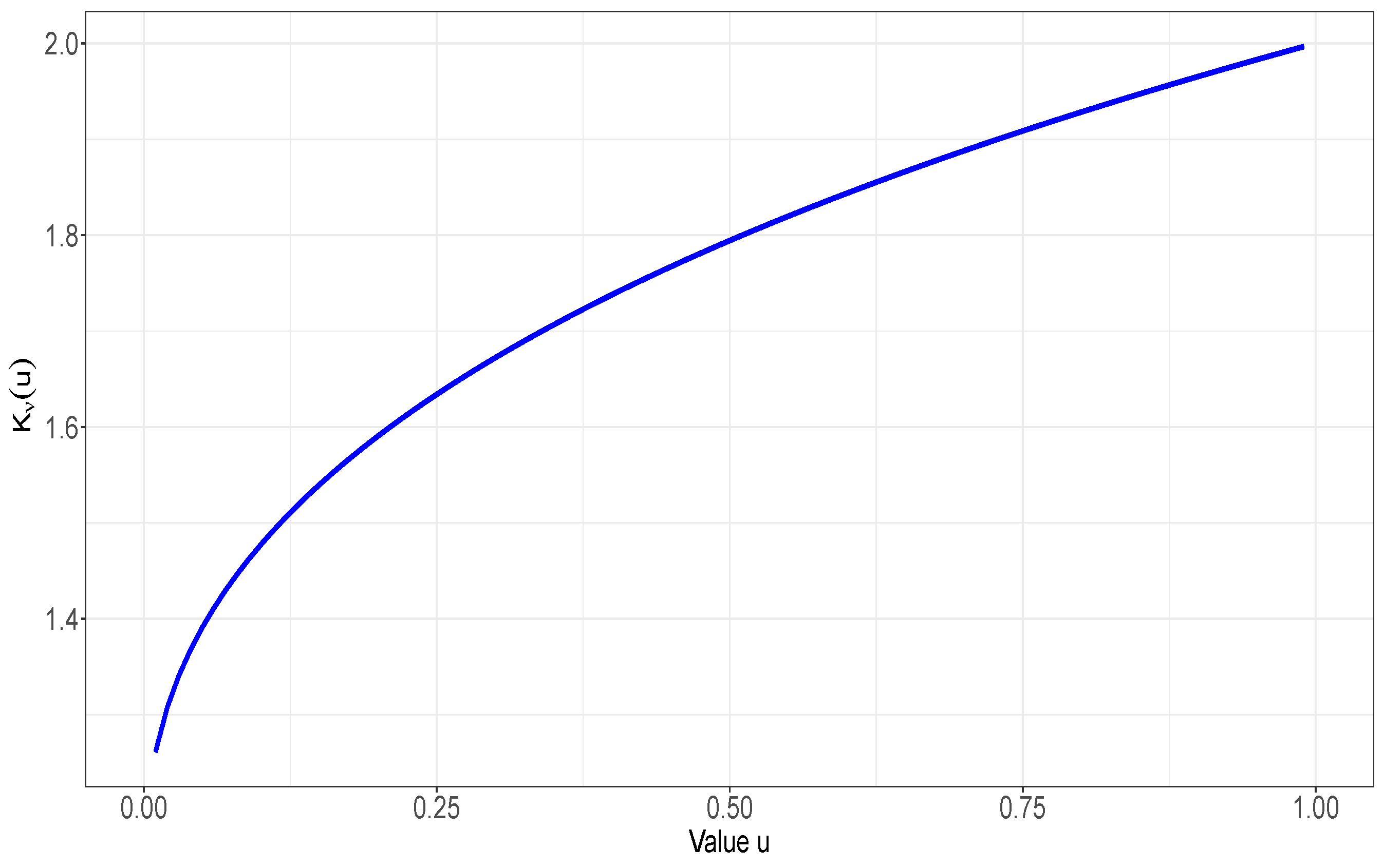
Suppose that

ν (u) = u exp (1 - u)

, which is distortion function. It is seen that

Φ (x) = 1 - x .

Thus,

\frac{Φ (x^{α})}{Φ (x)} = \frac{1 - x^{α}}{1 - x}

. From Lemma 2.2,

\frac{Φ (x^{α})}{Φ (x)}

is decreasing in

x \in [0, 1]

for every

α \in [0, 1]

. Therefore, according to Lemma 2.1,

K_{ν} (u) : = \frac{- ln (u) Φ (u)}{- ln (ν (u))} = \frac{- ln (u) . (1 - u)}{u - ln (u) - 1},

is increasing in

u \in [0, 1]

. We plot the graph of

K_{ν} (u)

for

u \in [0, 1]

in Figure .

Figure 1. Plot of

K_{ν} (u) : = \frac{- ln (u) . (1 - u)}{u - ln (u) - 1}

for

u \in [0, 1]

Figure 1. Plot of

K_{ν} (u) : = \frac{- ln (u) . (1 - u)}{u - ln (u) - 1}

for

u \in [0, 1]

The following proposition presents some sufficient condition under which “

\frac{Φ (x^{α})}{Φ (x)}

is decreasing (increasing) in

x \in (0, 1)

for every

α \in (0, 1)

”.

Proposition 2.4.

Let

Φ (x) : = \frac{x . ν^{'} (x)}{ν (x)}

is a differentiable function of

x \in [0, 1]

. Suppose the partial derivatives of

Φ (x^{α})

with respect x and α exist and are continuous in

x \in [0, 1]

and

α \in [0, 1]

. Let one of the following (equivalent) conditions hold:

(i): The function $ξ : {[0, 1]}^{2} \mapsto (0, + \infty)$ where $ξ (x, α) : = Φ (x^{α}),$ is $T P_{2}$ ( $R R_{2}$ ) in $(x, α) \in [0, 1] \times [0, 1] .$
(ii): For all $(x, α) \in {[0, 1]}^{2}$ , it holds that $\frac{\partial^{2}}{\partial α \partial x} ln (ξ (x, α)) \geq (\leq) 0$ .

Then,

\frac{Φ (x^{α})}{Φ (x)}

is decreasing (increasing) in

x \in [0, 1]

for every

α \in [0, 1]

Proof.

It is notable from Theorem 7.1 in Holland and Wang [12] that the assertions (i) and (ii) are equivalent. Therefore, we only show that assertion (i) implies that

\frac{Φ (x^{α})}{Φ (x)}

is decreasing (increasing) in

x \in [0, 1]

for all

α \in [0, 1]

. To this end, assume that

ξ (x, α)

T P_{2}

(

R R_{2}

) in

(x, α) \in {[0, 1]}^{2}

. Then,

ξ (x_{1}, α_{1}) . ξ (x_{2}, α_{2}) \geq (\leq) ξ (x_{1}, α_{2}) . ξ (x_{2}, α_{1}), f o r e v e r y x_{1} \leq x_{2} \in [0, 1] a n d, f o r a l l α_{1} \leq α_{2} \in [0, 1],

(2.5)

Let

α

be an arbitrary value in

[0, 1]

. In the particular case when

α_{1} = α

and

α_{2} = 1

, the inequality given in (2.5) gives

ξ (x_{1}, α) . ξ (x_{2}, 1) \geq (\leq) ξ (x_{1}, 1) . ξ (x_{2}, α), f o r a l l x_{1} \leq x_{2} \in [0, 1], a n d f o r a l l α \in [0, 1] .

(2.6)

Using the conventions

\frac{a}{0} = 0

for

a = 0

and

\frac{a}{0} = + \infty

for

a > 0

, it follows from (2.6) that

\frac{ξ (x_{1}, α)}{ξ (x_{1}, 1)} \geq (\leq) \frac{ξ (x_{2}, α)}{ξ (x_{2}, 1)}, f o r e v e r y x_{1} \leq x_{2} \in [0, 1], a n d f o r a l l α \in [0, 1] .

This is equivalent to saying that

\frac{ξ (x, α)}{ξ (x, 1)}

is decreasing (increasing) in

x \in [0, 1]

for all

α \in [0, 1]

. The required result is achieved. □ □

Theorem 2.5.

Let

Φ (u) = \frac{u . ν^{'} (u)}{ν (u)}

and let

\frac{Φ (x^{α})}{Φ (x)}

be decreasing in

x \in [0, 1]

for every

α \in [0, 1]

. If

X \geq_{s t} Y

, then

X \leq_{A I} Y ⟹ X_{ν} \leq_{A I} Y_{ν} .

(2.7)

Proof.

From assumption

X \leq_{A I} Y

. Using Theorem 3.1(iii) of Nanda et al. [26],

\frac{- ln (\bar{F} (t))}{- ln (\bar{G} (t))}

is increasing in

t \geq 0

. On the other hand, since for all

t \geq 0,

\frac{d}{d t} (\frac{- ln (\bar{F} (t))}{- ln (\bar{G} (t))}) \overset{s g n}{=} h_{X} (t) (- ln (\bar{G} (t))) - h_{Y} (t) (- ln (\bar{F} (t))),

thus if

\frac{- ln (\bar{F} (t))}{- ln (\bar{G} (t))}

is increasing in

t \geq 0

, then

\frac{h_{X} (t)}{h_{Y} (t)} \geq \frac{- ln (\bar{F} (t))}{- ln (\bar{G} (t))}, f o r a l l t \geq 0 .

(2.8)

To prove

X_{ν} \leq_{A I} Y_{ν}

, we show that

\frac{d}{d t} (\frac{- ln ({\bar{F}}_{ν} (t))}{- ln ({\bar{G}}_{ν} (t))}) \geq 0,

for all

t \geq 0

. We have

\begin{matrix} \frac{d}{d t} (\frac{- ln ({\bar{F}}_{ν} (t))}{- ln ({\bar{G}}_{ν} (t))}) & = \frac{d}{d t} (\frac{- ln (ν (\bar{F} (t)))}{- ln (ν (\bar{G} (t)))}) \\ \overset{s g n}{=} \frac{f (t) ν^{'} (\bar{F} (t))}{ν (\bar{F} (t))} (- ln (ν (\bar{G} (t)))) - \frac{g (t) ν^{'} (\bar{G} (t))}{ν (\bar{G} (t))} (- ln (ν (\bar{F} (t)))) . \end{matrix}

Therefore,

X_{ν} \leq_{A I} Y_{ν}

holds if, and only if,

h_{X} (t) Φ (\bar{F} (t)) (- ln (ν (\bar{G} (t)))) \geq h_{Y} (t) Φ (\bar{G} (t)) (- ln (ν (\bar{F} (t)))), f o r a l l t \geq 0 .

(2.9)

The inequality given in (2.9) is satisfied if, and only if,

\frac{h_{X} (t)}{h_{Y} (t)} \geq \frac{Φ (\bar{G} (t))}{Φ (\bar{F} (t))} . \frac{- ln (ν (\bar{F} (t)))}{- ln (ν (\bar{G} (t)))}, f o r a l l t \geq 0 .

(2.10)

From (2.8), the inequality given in (2.10) is satisfied when

\frac{- ln (\bar{F} (t))}{- ln (\bar{G} (t))} \geq \frac{Φ (\bar{G} (t))}{Φ (\bar{F} (t))} . \frac{- ln (ν (\bar{F} (t)))}{- ln (ν (\bar{G} (t)))}, f o r a l l t \geq 0,

or equivalently if,

\frac{- ln (\bar{F} (t)) Φ (\bar{F} (t))}{- ln (ν (\bar{F} (t)))} \geq \frac{- ln (\bar{G} (t)) Φ (\bar{G} (t))}{- ln (ν (\bar{G} (t)))}, f o r a l l t \geq 0 .

(2.11)

From assumption,

X \geq_{s t} Y

which implies that

\bar{F} (t) \geq \bar{G} (t),

for all

t \geq 0

. Therefore, in order to demonstrate (2.11), it suffices to prove that

\frac{- ln (u) Φ (u)}{- ln (ν (u))}

is an increasing function in

u \in [0, 1]

. In view of the notation defined in Lemma 2.1, this is equivalent to saying that

K_{ν} (u)

is an increasing function in

u \in [0, 1]

. From assumption the result follows from Lemma 2.1 and the proof is complete. □ □

The following lemma is useful in the sequel.

Lemma 2.6.

For every

0 < a < b,

\frac{ln (1 + a t)}{ln (1 + b t)}

is increasing in

t > 0 .

Proof.

For every

t > 0,

let us write

\begin{matrix} \frac{ln (1 + a t)}{ln (1 + b t)} & = \frac{\int_{0}^{t} \frac{a}{1 + a x} d x}{\int_{0}^{t} \frac{b}{1 + b x} d x} \\ = \frac{W (2, t)}{W (1, t)}, \end{matrix}

where

W (j, t) : = \int_{0}^{\infty} γ (j, x) . I [x \leq t] d x, j = 1, 2; t > 0,

(2.12)

in which

I [x \leq t]

is the indicator function of the set

[x \leq t]

γ (j, x) = \frac{b}{1 + b x}

for

j = 1

and

γ (j, x) = \frac{a}{1 + a x}

whenever

j = 2

. It is straightforward to see that

γ (j, x)

T P_{2}

(j, x) \in {1, 2} \times (0, \infty)

and, further, one can check that

I [x \leq t]

T P_{2}

(x, t) \in (0, \infty) \times (0, \infty)

. Thus, applying general composition theorem of Karlin [17] to Eq. (2.12),

W (j, t)

T P_{2}

(j, t) \in {1, 2} \times (0, \infty)

. Hence,

\frac{W (2, t)}{W (1, t)}

is increasing in

t > 0

which completes the proof. □

Next, we give an example to show that Theorem 2.5 is applicable.

Example 2.7.

Suppose that X and Y have s.f.s

{\bar{F}}_{X} (t) = \frac{1}{{(1 + 2 t)}^{2}}, t \geq 0

and

{\bar{F}}_{Y} (t) = \frac{1}{{(1 + 4 t)}^{2}}, t \geq 0

. Assume that

ν (u) = u . exp (1 - u)

, and thus

X_{ν}

and

Y_{ν}

have respective s.f.s

{\bar{F}}_{X_{ν}} (t) = \frac{1}{{(1 + 2 t)}^{2}} . exp (\frac{4 t + 4 t^{2}}{{(1 + 2 t)}^{2}}) a n d {\bar{F}}_{Y_{ν}} (t) = \frac{1}{{(1 + 4 t)}^{2}} . exp (\frac{8 t + 16 t^{2}}{{(1 + 4 t)}^{2}}) .

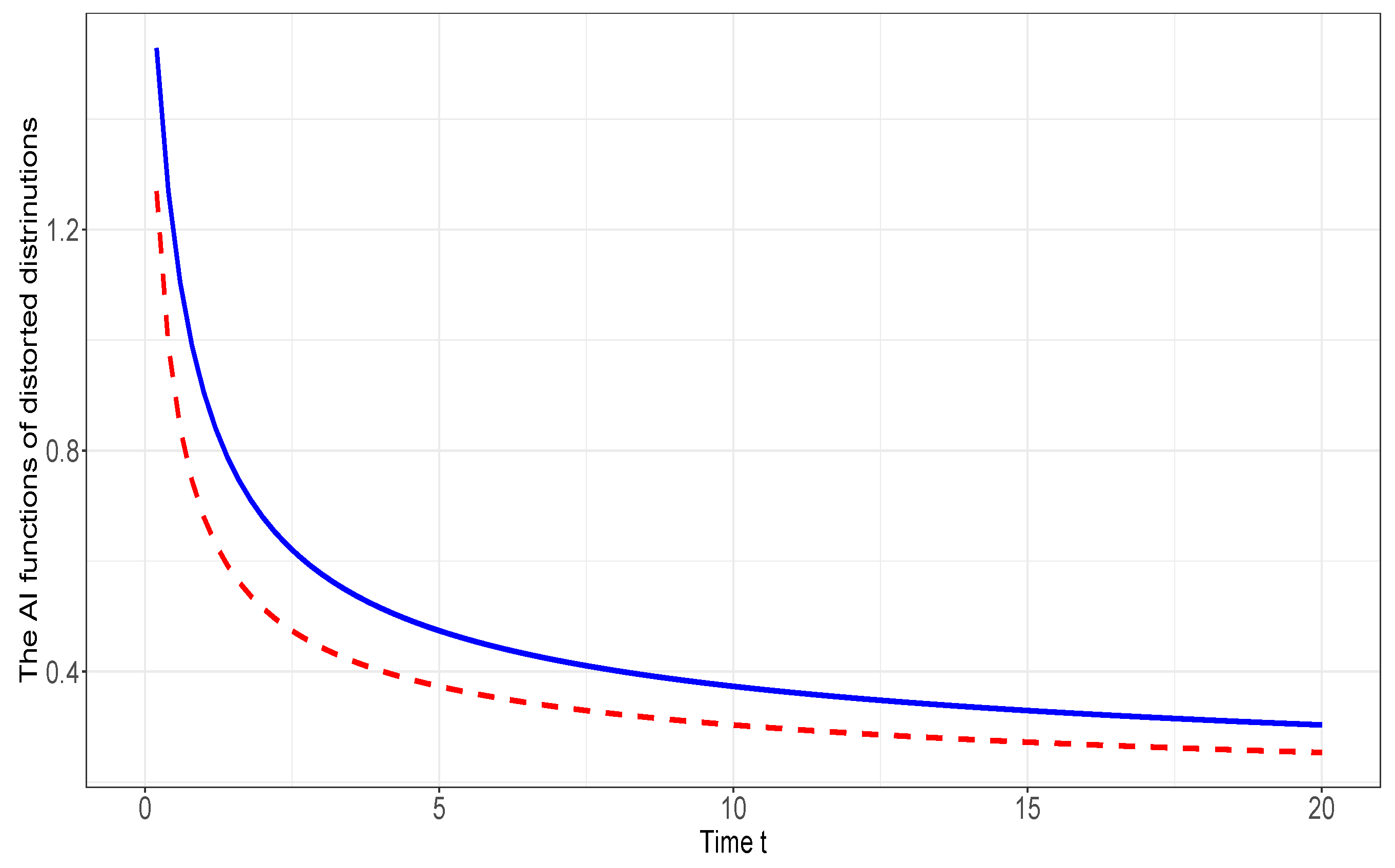
It is plainly seen that

X \geq_{s t} Y

. We have

\frac{ln ({\bar{F}}_{X} (t))}{ln ({\bar{F}}_{Y} (t))} = \frac{ln (1 + 2 t)}{ln (1 + 4 t)}

which by using Lemma 2.6, increases in

t > 0

. In view of Theorem 3.1 (i) and (iii) of Nanda et al. [26],

X \leq_{A I} Y

. From Example 2.3,

\frac{Φ (x^{α})}{Φ (x)}

is decreasing in

x \in [0, 1]

for every

α \in [0, 1]

. Therefore, by using Theorem 2.5, we deduce that

X_{ν} \leq_{A I} Y_{ν} .

Note that the

A I

functions of

X_{ν}

and

Y_{ν}

are given, respectively, by

L_{X_{ν}} (t) = \frac{16 (1 + t) t^{2}}{2 {(1 + 2 t)}^{3} ln (1 + 2 t) - 4 t (1 + t) (1 + 2 t)}

and

L_{Y_{ν}} (t) = \frac{64 (1 + 2 t) t^{2}}{2 {(1 + 4 t)}^{3} ln (1 + 4 t) - 8 t (1 + 4 t) (1 + 2 t)} .

In Figure , we plot the graph of

A I

functions of

X_{ν}

and

Y_{ν}

Figure 2. Plot of

A I

functions of

X_{ν}

(solid line) and

Y_{ν}

(dashed line)

Figure 2. Plot of

A I

functions of

X_{ν}

(solid line) and

Y_{ν}

(dashed line)

3. A Lower Bound for the Average Intensity Function

The following proposition presents an application of Theorem 2.5 to get a lower bound for the AI function of a distorted distribution under some condition on the base distribution.

Proposition 3.1.

Let X have the

I F R A

property such that

h_{X} (\infty) = m

. Suppose ν is a distortion function such that

\frac{Φ (x^{α})}{Φ (x)}

is decreasing in

x \in [0, 1]

for all

α \in [0, 1] .

Then,

L_{X_{ν}} (t) \geq \frac{m t e^{- m t} ν^{'} (e^{- m t})}{- ν (e^{- m t}) ln (ν (e^{- m t}))}, f o r a l l t \geq 0 .

(3.13)

Proof.

Define Y as an r.v. with exponential distribution with mean

\frac{1}{m}

. It is observed, after routine calculation, that

L_{Y} (t) = 1,

for all

t \geq 0

. On the other hand, X is

I F R A

if, and only if,

L_{X} (t) \geq 1,

for all

t \geq 0

. Thus, we deduce that

L_{X} (t) \geq L_{Y} (t),

for all

t \geq 0,

i.e.,

X \leq_{A I} Y

. Since X is

I F R A

, thus for all

t > 0,

\begin{matrix} \frac{- ln (\bar{F} (t))}{t} & = \frac{\int_{0}^{t} h_{X} (s) d s}{t} \\ \leq lim_{t \to \infty} \frac{\int_{0}^{t} h_{X} (s) d s}{t} \\ = h_{X} (\infty) . \end{matrix}

Therefore,

\frac{- ln (\bar{F} (t))}{t} \leq m

, for all

t \geq 0

, or equivalently,

\bar{F} (t) \geq e^{- m t},

for every

t \geq 0 .

This means

X \geq_{s t} Y

. From assumption

\frac{Φ (x^{α})}{Φ (x)}

is decreasing in

x \in [0, 1]

for every

α \in [0, 1]

. By using Theorem 2.5, one concludes

X_{ν} \leq_{A I} Y_{ν}

which reveals that

L_{X_{ν}} (t) \geq L_{Y_{ν}} (t), f o r a l l t \geq 0 .

(3.14)

Denote by

h_{Y_{ν}}

and

{\bar{G}}_{ν}

the h.r.f. and the s.f. of

Y_{ν}

. Note that

{\bar{G}}_{ν} (t) = ν (e^{- m t})

. We get

\begin{matrix} L_{Y_{ν}} (t) & = \frac{t h_{Y_{ν}} (t)}{- ln ({\bar{G}}_{ν} (t))} \\ = \frac{t . \frac{- \partial}{\partial t} ln (ν (e^{- m t}))}{- ln (ν (e^{- m t}))} \\ = \frac{m t e^{- m t} ν^{'} (e^{- m t})}{- ν (e^{- m t}) ln (ν (e^{- m t}))} . \end{matrix}

Now, the proof follows from (3.14). □

The next example presents a lower bound for the

A I

function of the lifetime of a parallel system with components’ lifetime having the

I F R A

property.

Example 3.2.

Consider a parallel system with independent components’ lifetimes

X_{1}, X_{2}, \dots, X_{n}

with a common s.f.

\bar{F}

. The lifetime of the system is

X_{n : n},

the maximum order statistic of

X_{1}, X_{2}, \dots, X_{n}

, which has s.f.

{\bar{F}}_{X_{n : n}} (t) = ν (\bar{F} (t))

, where

ν (u) = 1 - {(1 - u)}^{n} .

Using the identity

1 - {(1 - x)}^{n} = x \sum_{j = 0}^{n - 1} {(1 - x)}^{j}

, for all

x \in (0, 1),

we get

\begin{matrix} Φ (x) & = \frac{x . ν^{'} (x)}{ν (x)} \\ = \frac{n x {(1 - x)}^{n - 1}}{1 - {(1 - x)}^{n}} \\ = \frac{n {(1 - x)}^{n - 1}}{\sum_{j = 0}^{n - 1} {(1 - x)}^{j}} \\ = \frac{n}{\sum_{j = 0}^{n - 1} {(1 - x)}^{j - n + 1}} . \end{matrix}

Now, one can observe that

\begin{matrix} \frac{Φ (x^{α})}{Φ (x)} & = \frac{\sum_{j = 0}^{n - 1} {(1 - x)}^{j - n + 1}}{\sum_{j = 0}^{n - 1} {(1 - x^{α})}^{j - n + 1}} \\ = \sum_{j = 0}^{n - 1} {(\frac{1 - x}{1 - x^{α}})}^{j - n + 1} . \frac{{(1 - x^{α})}^{j - n + 1}}{\sum_{j = 0}^{n - 1} {(1 - x^{α})}^{j - n + 1}} \\ = \sum_{j = 0}^{n - 1} ω (j; x) . f (j ∣ x) \\ = E [ω (J_{x}; x)], \end{matrix}

where

ω (j; x) : = {(\frac{1 - x}{1 - x^{α}})}^{j - n + 1}

and

J_{x}

is a discrete r.v. with probability mass function

f (j ∣ x)

given by

f (j ∣ x) : = \frac{{(1 - x^{α})}^{j - n + 1}}{\sum_{j = 0}^{n - 1} {(1 - x^{α})}^{j - n + 1}}, j = 0, 1, \dots, n - 1 .

(3.15)

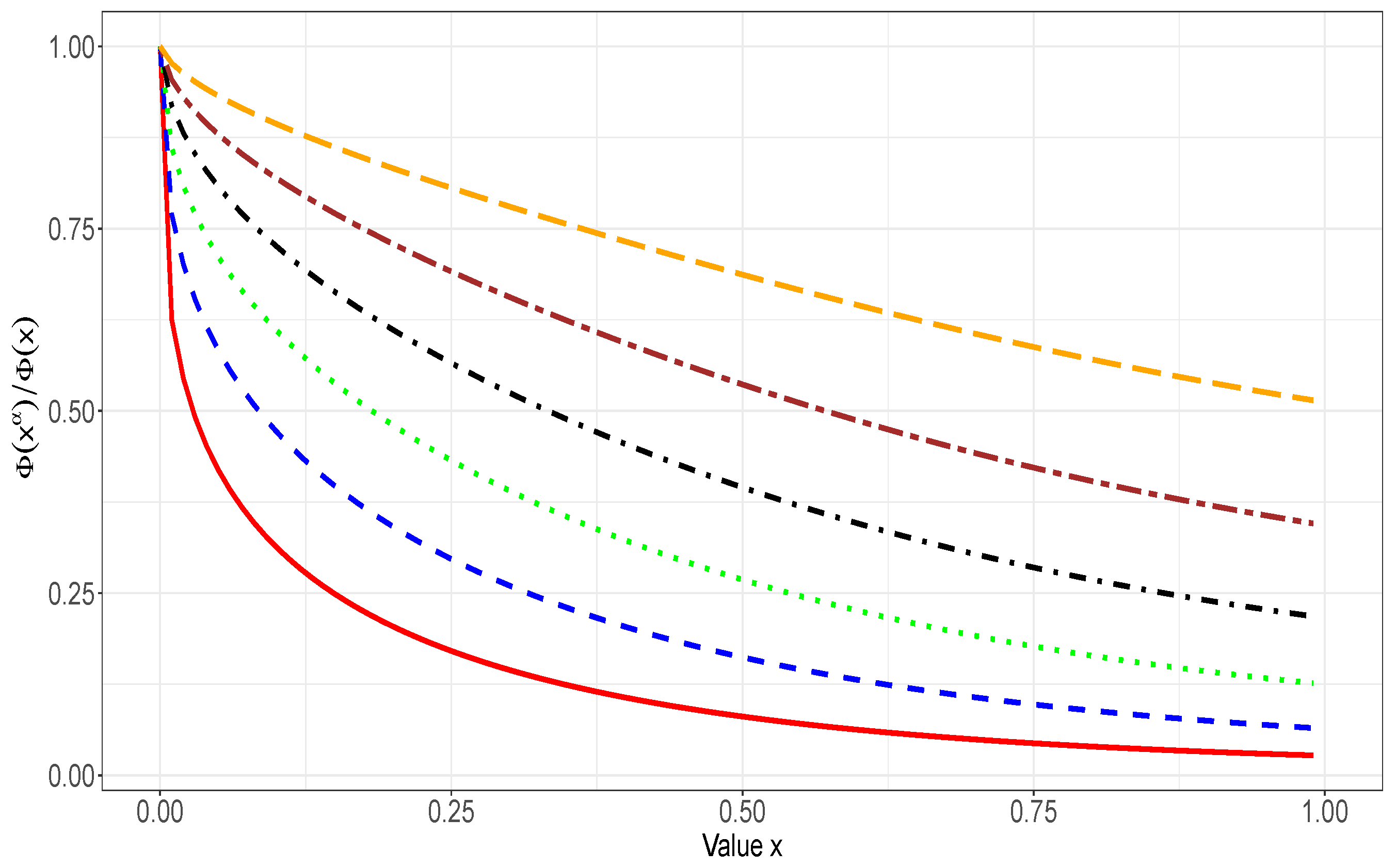
Since

j - n + 1 \leq 0

, for all

j = 0, 1, \dots, n,

thus using Lemma 2.2,

ω (j; x)

is decreasing in

x \in (0, 1),

for every

j = 0, 1, \dots, n

. On the other hand, since for all

x \in (0, 1)

and for every

α \in [0, 1]

\frac{1 - x}{1 - x^{α}} \geq 1

, thus,

ω (j; x)

is increasing in

j = 0, 1, \dots, n

for every

x \in (0, 1)

. It is also obvious from (3.15) that

\frac{f (j_{2} ∣ x)}{f (j_{1} ∣ x)}

is decreasing in

x \in (0, 1)

which means that

J_{x_{1}} \geq_{l r} J_{x_{2}},

for all

x_{1} \leq x_{2} \in (0, 1)

. Therefore,

J_{x}

is stochastically decreasing in

x \in (0, 1)

. Now, by using Lemma 2.2(ii) of Misra and van der Meulen [23],

E [ω (J_{x}; x)]

and, consequently,

\frac{Φ (x^{α})}{Φ (x)}

is decreasing in

x \in [0, 1]

. The graph of

\frac{Φ (x^{α})}{Φ (x)}

has been plotted in Figure for some choices of

α \in (0, 1)

. Note that the right hand side expression in Eq. (3.13) in Proposition 3.1 is obtained as

\begin{matrix} \frac{m t e^{- m t} ν^{'} (e^{- m t})}{- ν (e^{- m t}) ln (ν (e^{- m t}))} & = \frac{n m t e^{- m t} {(1 - e^{- m t})}^{n - 1}}{- ln (1 - {(1 - e^{- m t})}^{n}) (1 - {(1 - e^{- m t})}^{n})} \\ = \frac{n m t}{- ln (1 - {(1 - e^{- m t})}^{n}) . \sum_{j = 0}^{n - 1} {(1 - e^{- m t})}^{j - n + 1}} \\ = \frac{n t {[\sum_{j = 0}^{n - 1} {(1 - e^{- m t})}^{j - n + 1}]}^{- 1}}{t - ln {(\sum_{j = 0}^{n - 1} {(1 - e^{- m t})}^{j})}^{\frac{1}{m}}}, \end{matrix}

where the identity

1 - {(1 - e^{- m t})}^{n} = e^{- m t} . \sum_{j = 0}^{n - 1} {(1 - e^{- m t})}^{j}

is utilized. Now, let us assume that the lifetime of the components of the parallel system have the

I F R A

property such that

h_{X_{1}} (\infty) = m

. Therefore, by using Proposition 3.1, we have:

L_{X_{n : n}} (t) \geq \frac{n t {[\sum_{j = 0}^{n - 1} {(1 - e^{- m t})}^{j - n + 1}]}^{- 1}}{t - ln {(\sum_{j = 0}^{n - 1} {(1 - e^{- m t})}^{j})}^{\frac{1}{m}}}, f o r a l l t \geq 0 .

(3.16)

Figure 3. Plot of

\frac{Φ (x^{α})}{Φ (x)}

for

α = 0.3, 0.4, 0.5, 0.6, 0.7

and

0.8

from bottom to up

Figure 3. Plot of

\frac{Φ (x^{α})}{Φ (x)}

for

α = 0.3, 0.4, 0.5, 0.6, 0.7

and

0.8

from bottom to up

The following example applies the materials in Example 3.2 in the case of a parametric distribution.

Example 3.3.

We consider a system with the parallel structure with three independent components’ lifetimes

(n = 3)

following common s.f.

{\bar{F}}_{X_{1}} (t) = {(1 + θ_{1} t)}^{\frac{θ_{2}}{θ_{1}^{2}}} . exp (- \frac{θ_{2}}{θ_{1}} t), t \geq 0

where

θ_{1} \in [0, 1]

and

θ_{2} > 0

. It can be seen that the h.r. of

X_{1}

h_{X_{1}} (t) = \frac{θ_{2} t}{1 + θ_{1} t}

which is increasing in

t \geq 0

, i.e. X is

I F R

and hence

I F R A

. It is obviously seen that

m = h_{X_{1}} (\infty) = \frac{θ_{2}}{θ_{1}}

. It can be verified that

L_{X_{3 : 3}} (t) = \frac{θ_{2} t^{2} {\bar{F}}_{X_{1}} (t) {(1 - {\bar{F}}_{X_{1}} (t))}^{2}}{- (1 + θ_{1} t) (1 - {(1 - {\bar{F}}_{X_{1}} (t))}^{3}) ln (1 - {(1 - {\bar{F}}_{X_{1}} (t))}^{3})} .

In view of the inequality (3.16),

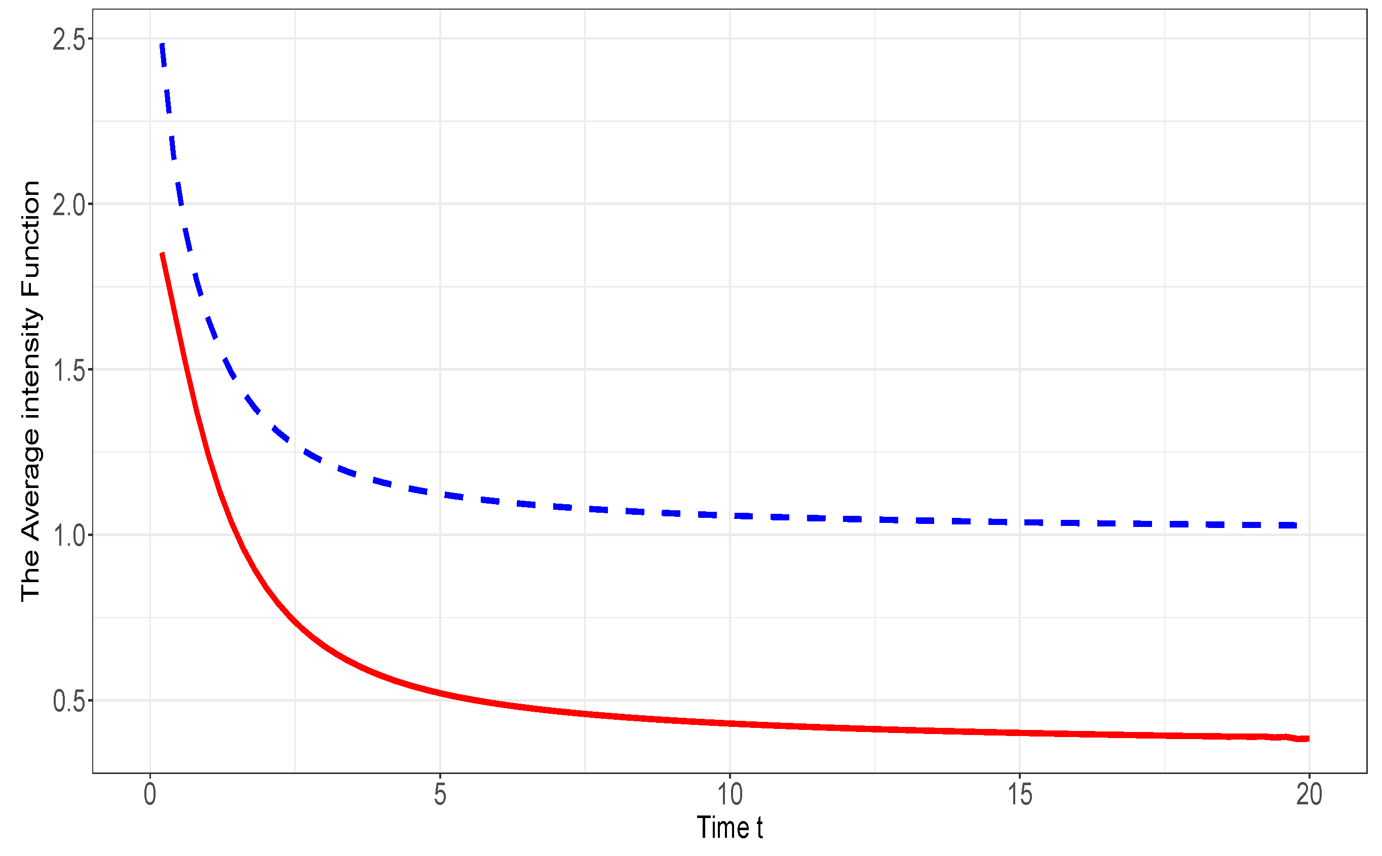
L_{X_{3 : 3}} (t) \geq \frac{3 t {[\sum_{j = 0}^{2} {(1 - e^{- \frac{θ_{2}}{θ_{1}} t})}^{j - 2}]}^{- 1}}{t - ln {(\sum_{j = 0}^{2} {(1 - e^{- \frac{θ_{2}}{θ_{1}} t})}^{j})}^{\frac{θ_{1}}{θ_{2}}}}, f o r a l l t \geq 0 .

In order to verify this, the graph of

L_{X_{3 : 3}} (t)

and also the function

\frac{3 t {[\sum_{j = 0}^{2} {(1 - e^{- \frac{θ_{2}}{θ_{1}} t})}^{j - 2}]}^{- 1}}{t - ln {(\sum_{j = 0}^{2} {(1 - e^{- \frac{θ_{2}}{θ_{1}} t})}^{j})}^{\frac{θ_{1}}{θ_{2}}}}

has been depicted in Figure for values

θ_{1} = 1

and

θ_{2} = 2

Figure 4. Plot of the

A I

function of

X_{3 : 3}

(dashed line) and its lower bound (solid line) in Example for

θ_{1} = 1

and

θ_{2} = 2

Figure 4. Plot of the

A I

function of

X_{3 : 3}

(dashed line) and its lower bound (solid line) in Example for

θ_{1} = 1

and

θ_{2} = 2

4. Preservation of the Increasing (Decreasing) Average Intensity Classes

In this subsection, we study the preservation of two aging classes of lifetime distributions under distortion. Through such an investigation, one may be able to translate stochastic aspects in original data into the same stochastic trends for transformed data following a distorted distribution. For example, in the context of a coherent system, the lifetime of its identical (possibly dependnet) components,

X_{1}, X_{2}, \dots, X_{n}

, can be anticipated as a potential for original data and the lifetime of the coherent system (

T = ϕ (X_{1}, X_{2}, \dots, X_{n})

) provides a transformation of the original data which follows a distorted distribution (see, for example, Navarro et al. [28], Izadkhah et al. [13] and Badía et al. [2]).

Next, we state the following result in which a similar sufficient condition as in Theorem 2.5 is considered.

Theorem 4.1.

Let

Φ (u) : = \frac{u . ν^{'} (u)}{ν (u)}

such that

\frac{Φ (x^{α})}{Φ (x)}

be increasing (resp. decreasing) in

x \in [0, 1]

for every

α \in [0, 1]

. Then,

X \in I A I (r e s p . X \in D A I) ⟹ X_{ν} \in I A I (r e s p . X_{ν} \in D A I) .

(4.17)

Proof.

We only prove the non-parenthetical part as the proof of the parenthetical part is similar. From Definition 1.2, it is sufficient to show that

L_{X_{ν}} (t)

is increasing in

t \geq 0

. Note that

\begin{matrix} h_{X_{ν}} (t) & = - \frac{d}{d t} ln (ν (\bar{F} (t))) \\ = \frac{ν^{'} (\bar{F} (t)) f (t)}{ν (\bar{F} (t))} \\ = \frac{\bar{F} (t) ν^{'} (\bar{F} (t))}{ν (\bar{F} (t))} . h_{X} (t) \\ = Φ (\bar{F} (t)) . h_{X} (t), f o r a l l t \geq 0 . \end{matrix}

Now, we can develop the aging intensity function of

X_{ν}

as follows:

\begin{matrix} L_{X_{ν}} (t) & = \frac{t ν^{'} (\bar{F} (t)) \bar{F} (t) h_{X} (t)}{- ν (\bar{F} (t)) ln (ν (\bar{F} (t)))} \\ = \frac{- ν^{'} (\bar{F} (t)) \bar{F} (t) ln (\bar{F} (t))}{- ν (\bar{F} (t)) ln (ν (\bar{F} (t)))} . \frac{t h_{X} (t)}{- ln (\bar{F} (t))} \\ = \frac{- ν^{'} (\bar{F} (t)) \bar{F} (t) ln (\bar{F} (t))}{- ν (\bar{F} (t)) ln (ν (\bar{F} (t)))} . L_{X} (t), f o r a l l t \geq 0 . \end{matrix}

Therefore, if

X \in I A I

and if, further,

\frac{- ν^{'} (\bar{F} (t)) \bar{F} (t) ln (\bar{F} (t))}{- ν (\bar{F} (t)) ln (ν (\bar{F} (t)))} i s i n c r e a s i n g i n t \geq 0,

(4.18)

then

X_{ν} \in I A I

. The expression in (4.18) holds true if, and only if,

\frac{- u ν^{'} (u) ln (u)}{- ν (u) ln (ν (u))}

is decreasing in

u \in [0, 1]

. Given the notations of Lemma 2.1, this is equivalent to saying that

K_{ν} (u)

is decreasing in

u \in [0, 1] .

From assumption and also using the parenthetical part of Lemma 2.1, the result follows. □ □

The following example illustrates a situation where Theorem 4.1 is utilized.

Example 4.2.

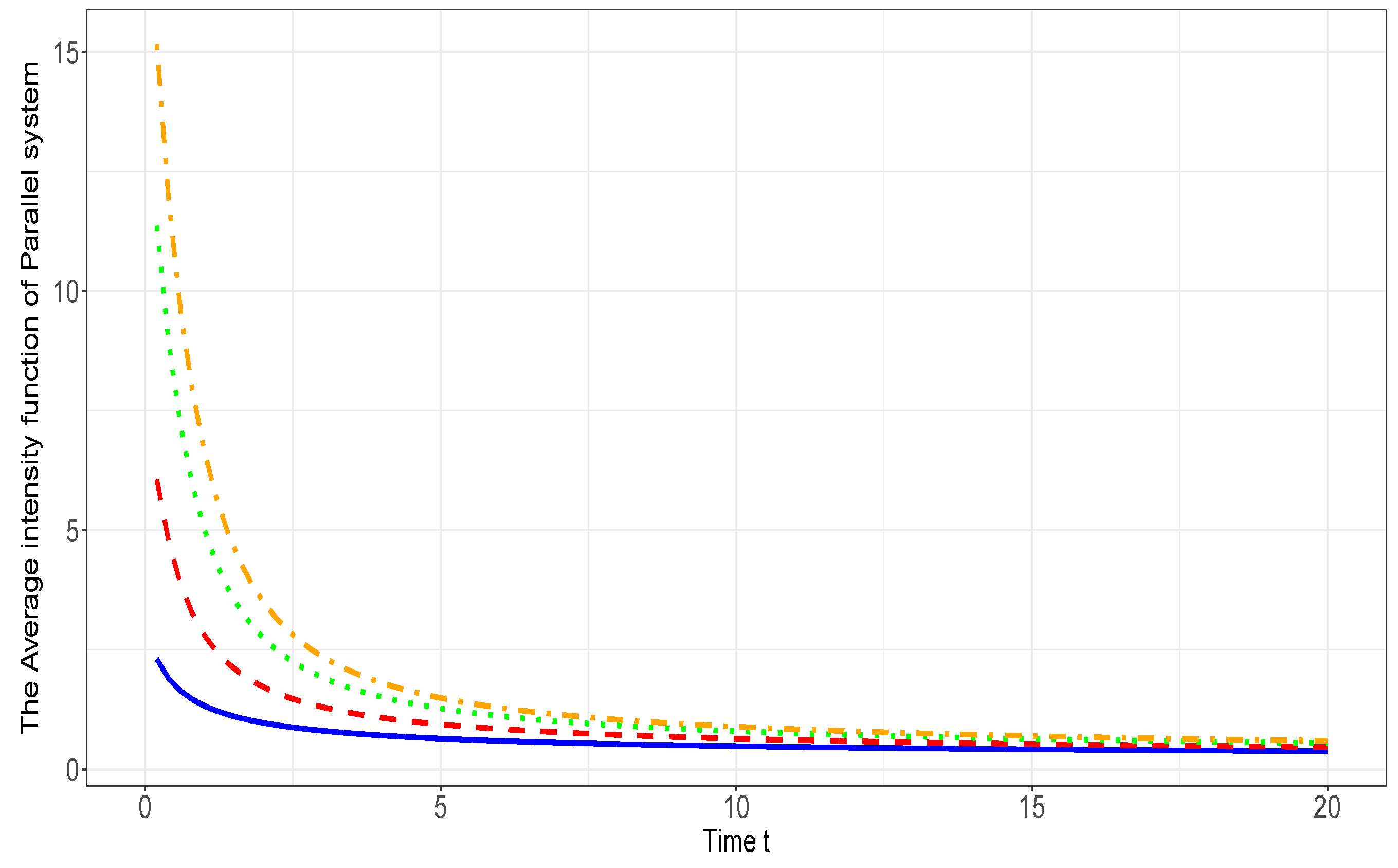
Consider a parallel system with independent component’s lifetime

X_{i}, i = 1, 2, \dots, n

following common s.f.

\bar{F} (t) = \frac{1}{{(1 + t)}^{2}}, t \geq 0

. It is seen that

- ln (\bar{F} (t)) = 2 ln (1 + t)

and thus

h_{X_{1}} (t) = \frac{2}{(1 + t)} .

Therefore, the

A I

function of

X_{1}

is given by

L_{X_{1}} (t) = \frac{t}{(1 + t) ln (1 + t)} .

Clearly,

X_{1}

has the

D A I

property if, and only if,

ψ (t) : = (1 + \frac{1}{t}) . ln (1 + t)

is increasing in

t \geq 0

. We can see that

ψ^{'} (t) \overset{s g n}{=} 1 - \frac{ln (1 + t)}{t}

which is non-negative for all

t \geq 0

because

ln (1 + t) \leq t,

for all

t \geq 0

. From Example 3.2,

\frac{Φ (x^{α})}{Φ (x)}

is decreasing in

x \in [0, 1]

. Thus, according to the parenthetical part of Theorem 4.1,

X_{n : n}

has the

D A I

property. The

A I

function of

X_{n : n}

can be acquired as

L_{X_{n : n}} (t) = \frac{2 n {(2 + t)}^{n - 1} t^{n}}{[{(1 + 2 t)}^{2 n + 1} - (1 + t) {(2 t + t^{2})}^{n}] . [ln (1 - \frac{{(2 t + t^{2})}^{n}}{{(1 + t)}^{2 n}})]} .

(4.19)

In Figure , we plot the graph of

L_{X_{n : n}} (t)

in terms of t for some choices of the components’ number n. As exhibited in this graph the function

L_{X_{n : n}} (t)

is decreasing in

t \geq 0

Figure 5. Plot of the

A I

functions of

X_{3 : 3}

(solid line),

X_{8 : 8}

(dashed line),

X_{15 : 15}

(dotted line) and

X_{20 : 20}

(dotdash line) in Example

Figure 5. Plot of the

A I

functions of

X_{3 : 3}

(solid line),

X_{8 : 8}

(dashed line),

X_{15 : 15}

(dotted line) and

X_{20 : 20}

(dotdash line) in Example

5. Analysis of Semiparametric Models

Semiparametric families are particular distorted distributions for which the distortion function

ν

is characterized (see, e.g. Chapter 7 of Marshall and Olkin [22]). Closure properties of semiparametric families with respect to various stochastic orders and also preservation properties of stochastic orders under the structure of semiparametric families of distributions have been studied in literature (see, for instance, Navarro and del Águila [29], Kayid et al. [18], Burkschat and Navarro [7], Arriaza and Sordo [1] and Kayid and Al-Shehri [19]).

The following lemma which is useful to our destination, will be used in the sequel.

Lemma 5.1.

The following statements hold:

(i): Let $η \in (0, 1)$ (resp. $η \in (1, \infty)$ ) be an arbitrary value. Then,

${(1 - y)}^{η} \leq (\geq) 1 - η y, f o r a l l y \in [0, 1] .$
(ii): The function $d_{0} (y) : = \frac{(1 - y)}{\sqrt{y} . ln (y)}$ is increasing in $y \in (0, 1)$ .

Proof.

(i) .

To prove this assertion, let us denote

p_{η} (u) = {(1 - u)}^{η}

and

q_{η} (u) = 1 - η u

. Note that

p_{η} (1) = q_{η} (1) = 0,

for all

η \in (0, 1)

(resp.

η \in (1, \infty)

). One can get

p_{η}^{'} (u) = - η {(1 - u)}^{η - 1}

and

q_{η}^{'} (u) = - η

. It is obvious that, for all

η \in (0, 1)

(resp.

η \in (1, \infty)

), and for all

u \in (0, 1)

q_{η}^{'} (u) - p_{η}^{'} (u) = η . [{(1 - u)}^{η - 1} - 1] \geq (\leq) 0 .

For every

y \in (0, 1)

(resp.

η \in (1, \infty)

), it holds that:

q_{η} (y) - p_{η} (y) = \int_{0}^{y} (q_{η}^{'} (u) - p_{η}^{'} (u)) d u \geq (r e s p . \leq) 0 .

(i i) .

We first prove that

d_{1} (u) = d_{0} (u^{2})

is increasing in

u \in (0, 1)

. Then,

d_{0} (y) = d_{1} (\sqrt{y})

will be an increasing function of

y \in (0, 1)

. Note that

d_{1} (u) = \frac{u^{- 1} - u}{2 ln (u)} .

It can be seen that

d_{1}^{'} (u) \overset{s g n}{=} \frac{1}{2} (1 - \frac{1}{u^{2}} - (1 + \frac{1}{u^{2}}) ln (u)),

which is non-negative, if and only if,

- \frac{1}{2} ln (u^{2}) \geq \frac{1 - u^{2}}{1 + u^{2}}, f o r a l l u \in (0, 1) .

Therefore, it is enough to show that:

- \frac{1}{2} ln (w) \geq \frac{1 - w}{1 + w}, f o r a l l w \in (0, 1) .

(5.20)

Let us denote

k_{1} (s) : = - \frac{1}{2} ln (s)

and

k_{2} (s) : = \frac{1 - s}{1 + s}

. One has

k_{1} (1) = k_{2} (1) = 0

. Since

k_{1}^{'} (s) = - \frac{1}{2 s}

and

k_{2}^{'} (s) = - \frac{2}{{(1 + s)}^{2}}

, and because for all

s \in (0, 1)

, we have

{(1 - s)}^{2} \geq 0

, thus

k_{2}^{'} (s) - k_{1}^{'} (s) \geq 0,

for all

s \in (0, 1)

. Thus, for every

w \in (0, 1),

k_{1} (w) - k_{2} (w) = \int_{w}^{1} (k_{2}^{'} (s) - k_{1}^{'} (s)) d s \geq 0,

which proves the inequality in (5.20). The proof is completed. □ □

Below, we list a number of semiparametric families of distributions for which the results of this paper are fulfilled. The results of this paper (including Theorem 2.5, Proposition 2.4 and Theorem 4.1) consider a criterion on the distortion function

ν

in a general setting. For the case when

ν

is as arisen from the following typical semiparametric models, we shall establish the fulfillment of that criterion.

Proportional hazard rate model (PHRM)

The PHRM is a very well-known model in survival analysis (cf. Cox [8]). The idea is the proportionality of the hazard rate function of the distorted distribution

F_{ν}

with the hazard rate function of the underlying base distribution (F). Let us contemplate a non-negative r.v. X having s.f.

\bar{F}

. The r.v.

X_{ν}

with s.f.

{\bar{F}}_{X_{ν}} (t) = ν (\bar{F} (t))

where

ν (u) = u^{ξ},

with

ξ > 0

follows the PHRM. The PHRM is recognized by the following relationship:

h_{X_{ν}} (t) = ξ . h_{X} (t), f o r a l l t \geq 0,

where

h_{X_{ν}}

is the h.r. function of

X_{ν}

and

h_{X}

is the h.r. function of X. The parameter

ξ

is called the frailty parameter.

It is remarkable that the

A I

function is free of the frailty parameter

ξ

. This is because X and

X_{ν}

with

ν (u) = u^{ξ}

are identical in the

A I

function, i.e.,

L_{X_{ν}} (t) = L_{X} (t),

for all

t \geq 0

. On that account, it is clear that

X \leq_{A I} Y

is equivalent to

X_{ν} \leq_{A I} Y_{ν}

. In the context of Theorem 2.5,

Φ (x) = ξ,

for all

x \in [0, 1]

. Thus,

\frac{Φ (x^{α})}{Φ (x)} = 1

which is a constant function. Therefore, if

X \geq_{s t} Y

, then, the result of Theorem 2.5 holds. However, as discussed earlier, the result holds even without X being stochastically greater than Y in the sense of the usual stochastic order. This is an indication that the condition “

X \geq_{s t} Y

” in Theorem 2.5 is not a necessary condition. In the setting of Theorem 4.1,

X \in I A I

(resp.

X \in D A I

) if, and only if,

X_{ν} \in I A I

(resp.

X_{ν} \in D A I

Proportional reversed hazard rate model (PRHRM)

This model is characterized via the proportionality of the reversed hazard rate function of the distorted distribution

F_{ν}

with that of base distribution (F). Suppose that X is a non-negative r.v. with c.d.f. F. Then, the r.v.

X_{ν}

with s.f.

{\bar{F}}_{X_{ν}} (t) = ν (\bar{F} (t))

where

ν (u) = 1 - {(1 - u)}^{η},

with

η > 0

is said to follow the PRHRM. The parameter

η

is called the resilience parameter. We demonstrate here that the sufficient conditions of the results obtained in this paper (Theorem 2.5, Proposition 2.4 and Theorem 4.1) involving the distortion function

ν

of the PRHRM, are satisfied for the PRHRM.

To be more specific, we present the following proposition:

Proposition 5.2.

(i) .

η \in (0, 1),

then

\frac{Φ (x^{α})}{Φ (x)}

is increasing in

x \in [0, 1]

for all

α \in [0, 1]

, and

(i i) .

η \in (1, \infty),

then

\frac{Φ (x^{α})}{Φ (x)}

is decreasing in

x \in [0, 1]

for all

α \in [0, 1]

, and

Proof.

Note that if

ν (x) = 1 - {(1 - x)}^{η}

, then for every

x \in (0, 1)

, we have:

Φ (x^{α}) = \frac{x^{α} . ν^{'} (x^{α})}{ν (x^{α})} = \frac{η x^{α} {(1 - x^{α})}^{η - 1}}{1 - {(1 - x^{α})}^{η}} .

From Proposition 3.1(ii), to prove the assertion (i) (assertion (ii)) of the proposition, it suffices to prove that

Ψ (α, x) : = \frac{\partial}{\partial x} ln (Φ (x^{α}))

is a decreasing (increasing) function in

α \in (0, 1),

for all

x \in [0, 1]

. It can be seen after routine calculations that, for all

x \in (0, 1)

and also for all

α \in (0, 1)

\begin{matrix} Ψ (α, x) & = \frac{α}{x} + \frac{α (1 - η) x^{α}}{x (1 - x^{α})} - \frac{α η x^{α}}{x (1 - x^{α}) ({(1 - x^{α})}^{- θ} - 1)} \\ = \frac{1}{x ln (x)} (ln (x^{α}) + \frac{(1 - η) ln (x^{α}) x^{α}}{(1 - x^{α})} - \frac{η x^{α} ln (x^{α})}{(1 - x^{α}) ({(1 - x^{α})}^{- θ} - 1)}) . \end{matrix}

Now, it can be plainly verified that

Ψ (α, x)

is decreasing (increasing) in

α \in (0, 1)

, for every

x \in (0, 1)

when the following function is decreasing (increasing) in

y \in (0, 1)

Ψ^{*} (y) = ln (y) + \frac{(1 - η) y ln (y)}{1 - y} - \frac{η y ln (y)}{(1 - y) ({(1 - y)}^{- η} - 1)} .

We can see now that

\begin{matrix} Ψ^{*} (y) & = \frac{- y ln (y)}{1 - y} . (η - 1 + \frac{η}{{(1 - y)}^{- η} - 1} - \frac{1 - y}{y}) \\ = \frac{- y ln (y)}{1 - y} . (η + \frac{η}{{(1 - y)}^{- η} - 1} - \frac{1}{y}) \\ = Ψ_{0}^{*} (y) . Ψ_{1}^{*} (y), \end{matrix}

where

Ψ_{0}^{*} (y) = \frac{- y ln (y)}{1 - y}

and

Ψ_{1}^{*} (y) = η + \frac{η}{{(1 - y)}^{- η} - 1} - \frac{1}{y}

. To prove

Ψ^{*} (y)

is decreasing in

y \in (0, 1)

, it is enough to show that

Ψ_{0}^{*} (y)

is non-negative and increasing in

y \in (0, 1)

and further

Ψ_{1}^{*} (y)

is non-positive and decreasing in

y \in (0, 1)

as we prove that it holds true when

η \in (0, 1)

. As for the case when

η \in (1, \infty)

, we need to prove that

Ψ^{*} (y)

is an increasing function in

y \in (0, 1)

. In this case one needs to prove that

Ψ_{0}^{*} (y)

and also

Ψ_{1}^{*} (y)

are non-negative and increasing in

y \in (0, 1)

. We only prove the case of assertion (i) as the other assertion can be analogously proved. In the spirit of Lemma 5.1(ii), one has

Ψ_{0}^{*} (y) = - \frac{\sqrt{y}}{d_{0} (y)}

. Since

d_{0}

is increasing in

y \in (0, 1)

, thus

Ψ_{0}^{*} (y)

is increasing in

y \in (0, 1)

and also clearly it is a non-negative function. Moreover, from the non-parenthetical part of Lemma 5.1, it follows that

Ψ_{1}^{*} (y)

is non-negative for every

y \in (0, 1) .

Therefore, we only need to show that

Ψ_{1}^{*} (y)

is a decreasing function in

y \in (0, 1) .

Now, for every

y \in (0, 1)

we have

\frac{d}{d y} Ψ_{1}^{*} (y) = \frac{1}{y^{2}} - \frac{η^{2} {(1 - y)}^{- (1 + η)}}{{({(1 - y)}^{- η} - 1)}^{2}},

which is non-positive if, and only if,

\frac{{(1 - y)}^{- \frac{η}{2}} - {(1 - y)}^{\frac{η}{2}}}{η} \geq {(1 - y)}^{- \frac{1}{2}} - {(1 - y)}^{\frac{1}{2}}, f o r a l l y \in (0, 1),

which by the change of variable as

u = 1 - y

, is equivalent to

\frac{u^{- \frac{η}{2}} - u^{\frac{η}{2}}}{η} \geq u^{- \frac{1}{2}} - u^{\frac{1}{2}}, f o r a l l u \in (0, 1) .

(5.21)

To prove that (5.21) holds, it is sufficient to demonstrate that

δ_{η} (u) : = \frac{u^{- \frac{η}{2}} - u^{\frac{η}{2}}}{η}

is decreasing in

η \in (0, 1)

. Note that

η = \frac{ln (u^{η})}{ln (u)}

. Hence,

δ_{η} (u) = \frac{1 - u^{η}}{\sqrt{u^{η}} ln (u^{η})} ln (u) .

Thus, by taking

y = u^{η} \in (0, 1)

, it is seen that

δ_{η} (u)

is decreasing in

η \in (0, 1)

if, and only if,

d_{0} (y) = \frac{1 - y}{\sqrt{y} ln (y)}

is increasing in

y \in (0, 1)

. This holds true from Lemma 5.1. The proof is complete. □ □

Now, using the main results of this paper together with Proposition 5.2 we get the following corollary:

Corollary 5.3.

Let X and Y are two non-negative r.v.s with s.f.s

\bar{F}

and

\bar{G},

respectively. Suppose that

X_{ν}

and

Y_{ν}

follow the PRHRM with a common resilience parameter

η > 0

. Then:

(i): Let $η \in (1, \infty)$ . If $X \leq_{A I} Y$ and $X \geq_{s t} Y,$ then $X_{ν} \leq_{A I} Y_{ν} .$
(ii): Let $η \in (1, \infty)$ . If $X \in D A I$ then $X_{ν} \in D A I .$
(iii): Let $η \in (0, 1)$ . If $X \in I A I$ then $X_{ν} \in I A I .$

Hazard power model (HPM)

The HPM is a less known model in reliability theory (cf. Marshall and Olkin [22]). In this model, the

A I

function of the distorted distribution (

F_{ν}

) and the

A I

function of the base distribution F are considered proportional. We contemplate a non-negative r.v. X following s.f.

\bar{F}

. The r.v.

X_{ν}

with s.f.

{\bar{F}}_{X_{ν}} (t) = ν (\bar{F} (t))

where

ν (u) = exp (- {(- ln (u))}^{ζ}),

with

ζ > 0

is then said to follow the HPM. The parameter

ζ

is called the hazard power parameter. We show that the distortion function based conditions which are present in Theorem 2.5, Proposition 2.4 and Theorem 4.1 are satisfied. According to the HPM, let

X_{ν}

have s.f.

{\bar{F}}_{ν} (t) = exp (- {(- ln (\bar{F} (t)))}^{ζ}), t \geq 0

. To derive the

A I

function of

X_{ν}

, we get

\begin{matrix} L_{X_{ν}} (t) & = \frac{t . {(- ln ({\bar{F}}_{X_{ν}} (t)))}^{'}}{- ln ({\bar{F}}_{X_{ν}} (t))} \\ = \frac{ζ t h_{X} (t) . {(- ln (\bar{F} (t)))}^{ζ - 1}}{{(- ln (\bar{F} (t)))}^{ζ}} \\ = ζ . L_{X} (t), f o r a l l t \geq 0 . \end{matrix}

Therefore, we get the preservation property of the

A I

order under the structure of the HPM. The result holds since X and

X_{ν}

with

ν (u) = exp (- {(- ln (u))}^{ζ})

are proportional in the

A I

function, i.e.,

L_{X_{ν}} (t) = ζ . L_{X} (t),

for all

t \geq 0

. Therefore, since

L_{X_{ν}} (t) - L_{Y_{ν}} (t) = ζ . (L_{X} (t) - L_{Y} (t))

, thus it is obvious that

X \leq_{A I} Y

is equivalent to

X_{ν} \leq_{A I} Y_{ν}

. In the framework of Theorem 2.5, we get

\begin{matrix} Φ (u) & = \frac{u . ν^{'} (u)}{ν (u)} \\ = \frac{ζ . {(- ln (u))}^{ζ - 1} exp (- {(- ln (u))}^{ζ})}{exp (- {(- ln (u))}^{ζ})} \\ = ζ {(- ln (u))}^{ζ - 1}, f o r a l l u \in (0, 1) . \end{matrix}

Thus,

\frac{Φ (x^{α})}{Φ (x)} = α^{ζ - 1}

which is a constant function. Consequently, if

X \geq_{s t} Y

then, the result of Theorem 2.5 is satisfied. Following the foregoing discussion, the result of Theorem 2.5 holds even if

X ≱_{s t} Y

. Based on Theorem 4.1, in the context of the HPM, we conclude that

X \in I A I

(resp.

X \in D A I

) if, and only if,

X_{ν} \in I A I

(resp.

X_{ν} \in D A I

6. Concluding Remarks

Let us consider a non-negative random variable X that indicates the original lifetime of a unit with the survival function

\bar{F} (t)

. Now consider a new environment in which units are inserted to create a new system with lifetime

X_{ν}

and survival function

ν (\bar{F} (t))

. Many families or models in reliability theory and survival analysis have the formation of a skewed or distorted distribution. Sequential (generalized) order statistics, which include both the order statistics of a random sample and the lower and upper records (k-records) of a sequence of random variables, have the general form of a distorted distribution. The lifetime of a coherent system with identical but possibly dependent components also has a distorted distribution.

In this paper, we firstly studied the preservation properties of the average intensity order under distorted distributions. For two units (components of two systems) with lifetimes X and Y, the derived preservation result states that if X is less than or equal to Y in the average intensity order (i.e., if

X \leq_{A I} Y

), then under an order condition for the distribution functions of X and Y and a condition for the distortion function

ν

, the random lifetime

X_{ν}

is less than or equal to the random lifetime

Y_{ν}

(i.e.,

X_{ν} \leq_{A I} Y_{ν}

). If X and Y have survival functions

\bar{F} (t)

and

\bar{G} (t)

respectively, then

X_{ν}

and

Y_{ν}

with the respective survival functions

ν (\bar{F} (t))

and

ν (\bar{G} (t))

can denote the lifetime of systems consisting of the components (coherent systems). The preservation of an order property between

\bar{F}

and

\bar{G}

under the transformations

\bar{F} (t) \mapsto ν (\bar{F} (t))

and

\bar{G} (t) \mapsto ν (\bar{G} (t))

can be advantageous. For example, if the identical components of a system with lifetimes

X_{1}, \dots, X_{n}

have a lower average intensity function over time than the identical components of another system with lifetimes

Y_{1}, \dots, Y_{n}

, then one may wonder whether the lifetime of the system consisting of the components with lifetimes

X_{i}

also has a lower average intensity function than the lifetime of the system consisting of the components with lifetimes

Y_{i}

. This can be a challenge for system designers who always assume that a system with better components must also be more reliable, but this is not necessarily the case. The conditions for the preservation properties presented in our results are easy to distinguish in order to separate the effect of the distortion function

ν

and the effect of the base survival functions

\bar{F}

and

\bar{G}

. Thus, if for a distortion function

ν

x^{α - 1} \frac{ν^{'} (x^{α}) ν (x)}{ν (x^{α}) ν^{'} (x)}

is decreasing in

x \in [0, 1]

for all

α \in [0, 1]

and, separately, if the survival functions of the base distributions satisfy the ordering criteria

\bar{F} (t) \geq \bar{G} (t),

for all

t \geq 0

, then

X \leq_{A I} Y

implies

X_{ν} \leq_{A I} Y_{ν}

. At first glance, the first condition for the distortion function

ν

seems to be a rough condition. However, we have given many examples, including the well-known family of semiparametric models and also a parallel system where

x^{α - 1} \frac{ν^{'} (x^{α}) ν (x)}{ν (x^{α}) ν^{'} (x)}

is monotonic in

x \in [0, 1]

for all

α \in [0, 1] .

Another aspect of the preservation result for the average intensity order is related to the conditions for the base distributions, i.e.

X \leq_{A I} Y

together with

X \geq_{s t} Y

, which in turn is an indication of the direction in which one system is better than the other. In this context, it should be noted that the average intensity ordering focuses on the concept of faster aging, while the usual stochastic ordering deals with the notion of comparison in terms of the magnitude of random variables. So being better in one sense does not guarantee that you are better in another sense.

Secondly, the preservation property of the aging intensity order was used to derive a lower bound for the average intensity function of a distribution with increasing failure rate in the average property. Since the aging intensity function analyzes the aging property quantitatively, the larger aging intensity corresponds to the stronger tendency of aging (see, e.g. Jiang et al. ([14])). In this context, a lower bound for the average intensity function of a unit showing a positive aging process (e.g.

I F R A

) can indicate the extent of aging of a unit. To obtain the lower bound,

x^{α - 1} \frac{ν^{'} (x^{α}) ν (x)}{ν (x^{α}) ν^{'} (x)}

must be decreasing in

x \in [0, 1]

for all

α \in [0, 1],

and furthermore, knowing the exact amount of the extreme hazard rate of the base distribution is also necessary toward our destination.

Thirdly, the preservation property of two aging classes, namely the increasing average intensity (IAI) class and the decreasing average intensity (DAI) class, was established under a distorted distribution. The sufficient condition presented in this preservation result is again based on the monotonicity of

x^{α - 1} \frac{ν^{'} (x^{α}) ν (x)}{ν (x^{α}) ν^{'} (x)}

x \in [0, 1]

for all

α \in [0, 1]

. This establishes a link between the usability of the paper’s results for certain distorted distributions. In the context of reliability theory, we have shown that a parallel system with independent and identically distributed component lifetimes satisfy the results presented in the paper. We have finally proved that the sufficient conditions required to obtain our results are available for some well-known semiparametric models. On that account, one of the goals of of the current study has been the study of closure properties of semi-parametric families with a common real-valued parameter with respect to the underlying base distribution.

In the future of this study, the comparative analysis undertaken in this paper can be further developed in some other meanings. For example, the order properties and the aging properties of a semiparametric distribution could be studied in terms of its real parameters. The derivation of such closure properties may be useful to identify other aspects of probability distributions in modeling life events.

Acknowledgments

This work was supported by Researchers Supporting Project number (RSP2024R392), King Saud University, Riyadh, Saudi Arabia

References

Arriaza, A.; Sordo, M.A. Preservation of some stochastic orders by distortion functions with application to coherent systems with exchangeable components. Applied Stochastic Models in Business and Industry 2021, 37, 303–317. [Google Scholar] [CrossRef]
Badía, F.G.; Cha, J.H.; Lee, H.; Sangüesa, C. Preservation of the log-concavity by Bernstein operator with an application to aging properties of a coherent system. Journal of Computational and Applied Mathematics 2024, 443, 115748. [Google Scholar] [CrossRef]
Barlow, R.E.; Proschan, F. (1975). Statistical theory of reliability and life testing, New York: Holt, Rinehart and Winston. [Google Scholar]
Belzunce, F.; Riquelme, C.M.; Mulero, J. (2015). An introduction to stochastic orders, Academic Press. [Google Scholar]
Bhattacharjee, S.; Misra, S.K. Reliability analysis using aging intensity function. Statistics and Probability Letters 2013, 83, 1364–1371. [Google Scholar] [CrossRef]
Bhattacharjee, S.; Mohanty, I.; Szymkowiak, M. Properties of aging functions and their means. Communications in Statistics-Simulation and Computation.
Burkschat, M.; Navarro, J. Stochastic comparisons of systems based on sequential order statistics via properties of distorted distributions. Probability in the Engineering and Informational Sciences 2018, 32, 246–274. [Google Scholar] [CrossRef]
Cox, D.R. Regression models and life-tables. Journal of the Royal Statistical Society: Series B (Methodological) 1972, 34, 187–202. [Google Scholar] [CrossRef]
Denuit, M.; Dhaene, J.; Goovaerts, M.J.; Kaas, R. Actuarial Theory for Dependent Risks. John Wiley and Sons. 2005.
Giri, R.L.; N. ; a A.K.; Dasgupta, M.; Misra, S.K.; Bhattacharjee, S. On aging intensity function of some Weibull models. Communications in Statistics-Theory and Methods 2023, 52, 227–262. [Google Scholar] [CrossRef]
Goovaerts, M.J.; Kaas, R.; Laeven, R.J. Decision principles derived from risk measures. Insurance: Mathematics and Economics 2010, 47, 294–302. [Google Scholar] [CrossRef]
Holl, P.W.; Wang, Y.J. Dependence function for continuous bivariate densities. Communications in Statistics-Theory and Methods 1987, 16, 863–876. [Google Scholar]
Izadkhah, S.; Amini-Seresht, E.; Balakrishnan, N. Preservation properties of some reliability classes by lifetimes of coherent and mixed systems and their signatures. Probability in the Engineering and Informational Sciences 2023, 37, 943–960. [Google Scholar] [CrossRef]
Jiang, R.; Ji, P.; Xiao, X. Aging property of unimodal failure rate models. Reliability Engineering and System Safety 2003, 79, 113–116. [Google Scholar] [CrossRef]
Jiang, R.; Qi, F.; Cao, Y. Relation between aging intensity function and WPP plot and its application in reliability modelling. Reliability Engineering and System Safety 2023, 229, 108894. [Google Scholar] [CrossRef]
Jiang, R.; Cao, Y.; Qi, F. An aging-intensity-function-based parameter estimation method on heavily censored data. Quality and Reliability Engineering International 2023, 39, 3484–3501. [Google Scholar] [CrossRef]
Karlin, S. Total Positivity, Stanford University Press, 1968.
Kayid, M.; Izadkhah, S.; Alfifi, A. (2018). Increasing mean inactivity time ordering: a quantile approach. Mathematical Problems in Engineering, 2018. [Google Scholar]
Kayid, M.; Al-Shehri, M.A. Preservation of transform orders under a semiparametric model and its mixture. Operations Research Letters 2022, 50, 160–167. [Google Scholar] [CrossRef]
Lai, C.; Xie, M. (2006). Stochastic ageing and dependence for reliability, New York: Springer. [Google Scholar]
Li, H.; Li, X. (2013). Stochastic orders in reliability and risk. In: Honor of Professor Moshe Shaked. In: Lecture Notes in Statistics-Proceedings, Springer, New York.
Marshall, A.W.; Olkin, I. (2007). Life distributions, Springer, New York. [Google Scholar]
Misra, N.; van der Meulen, E.C. On stochastic properties of m-spacings. Journal of Statistical Planning and Inference 2003, 115, 683–697. [Google Scholar] [CrossRef]
Misra, S.K.; Bhattacharjee, S. A case study of aging intensity function on censored data. Alexandria engineering journal 2018, 57, 3931–3952. [Google Scholar] [CrossRef]
Müller, A.; Stoyan, D. (2002). Comparison Methods for Stochastic Models and Risks, Wiley, New York. [Google Scholar]
Nanda, A.K.; Bhattacharjee, S.; Alam, S.S. Properties of aging intensity function. Statistics and probability letters 2007, 77, 365–373. [Google Scholar] [CrossRef]
Navarro, J.; del Aguila, Y.; Sordo, M.A.; Suárez-Llorens, A. Stochastic ordering properties for systems with dependent identically distributed components. Applied Stochastic Models in Business and Industry 2013, 29, 264–278. [Google Scholar] [CrossRef]
Navarro, J.; del Águila, Y.; Sordo, M.A.; Suárez-Llorens, A. Preservation of reliability classes under the formation of coherent systems. Applied Stochastic Models in Business and Industry 2014, 30, 444–454. [Google Scholar] [CrossRef]
Navarro, J.; del Águila, Y. Stochastic comparisons of distorted distributions, coherent systems and mixtures with ordered components. Metrika 2017, 80, 627–648. [Google Scholar] [CrossRef]
Quiggin, J. A theory of anticipated utility. Journal of economic behavior and organization 1982, 3, 323–343. [Google Scholar] [CrossRef]
Rasin, R.S.; Sunoj, S.M.; Poduval, R. Kernel-based Estimation of Ageing Intensity Function: Properties and Applications. Austrian Journal of Statistics 2023, 52, 16–33. [Google Scholar] [CrossRef]
Raymarakkar, Sidhiq, R.; Sunoj, S.M.; Szymkowiak, M. Nonparametric estimation of aging intensity function for right-censored dependent data. J. Stat. Comput. Simul.
Schmeidler, D. Subjective probability and expected utility without additivity. Econom. J. Econom. Soc. 1989, 571–587. [Google Scholar] [CrossRef]
Shaked, M.; Shanthikumar, J.G. (Eds.). (2007). Stochastic orders. New York, NY: Springer New York.
Szymkowiak, M. Characterizations of distributions through aging intensity. IEEE Trans. Reliab. 2018, 67, 446–458. [Google Scholar] [CrossRef]
Yaari, M.E. The dual theory of choice under risk. Econom. J. Econom. Soc. 1987, 95–115. [Google Scholar] [CrossRef]

Disclaimer/Publisher’s Note: The statements, opinions and data contained in all publications are solely those of the individual author(s) and contributor(s) and not of MDPI and/or the editor(s). MDPI and/or the editor(s) disclaim responsibility for any injury to people or property resulting from any ideas, methods, instructions or products referred to in the content.

© 2024 by the authors. Licensee MDPI, Basel, Switzerland. This article is an open access article distributed under the terms and conditions of the Creative Commons Attribution (CC BY) license (http://creativecommons.org/licenses/by/4.0/).

Copyright: This open access article is published under a Creative Commons CC BY 4.0 license, which permit the free download, distribution, and reuse, provided that the author and preprint are cited in any reuse.

MDPI Initiatives

Important Links

Choose an area of interest and we will send you notifications of new preprints at your preferred frequency.

Disclaimer

Reliability Analysis of Distorted Distributions using Aging Intensity Function

Abstract

1. Introduction and Preliminaries

2. Preservation of the Average Intensity Order Under Distortion

3. A Lower Bound for the Average Intensity Function

4. Preservation of the Increasing (Decreasing) Average Intensity Classes

5. Analysis of Semiparametric Models

6. Concluding Remarks

Acknowledgments

References

MDPI Initiatives

Important Links

Subscribe