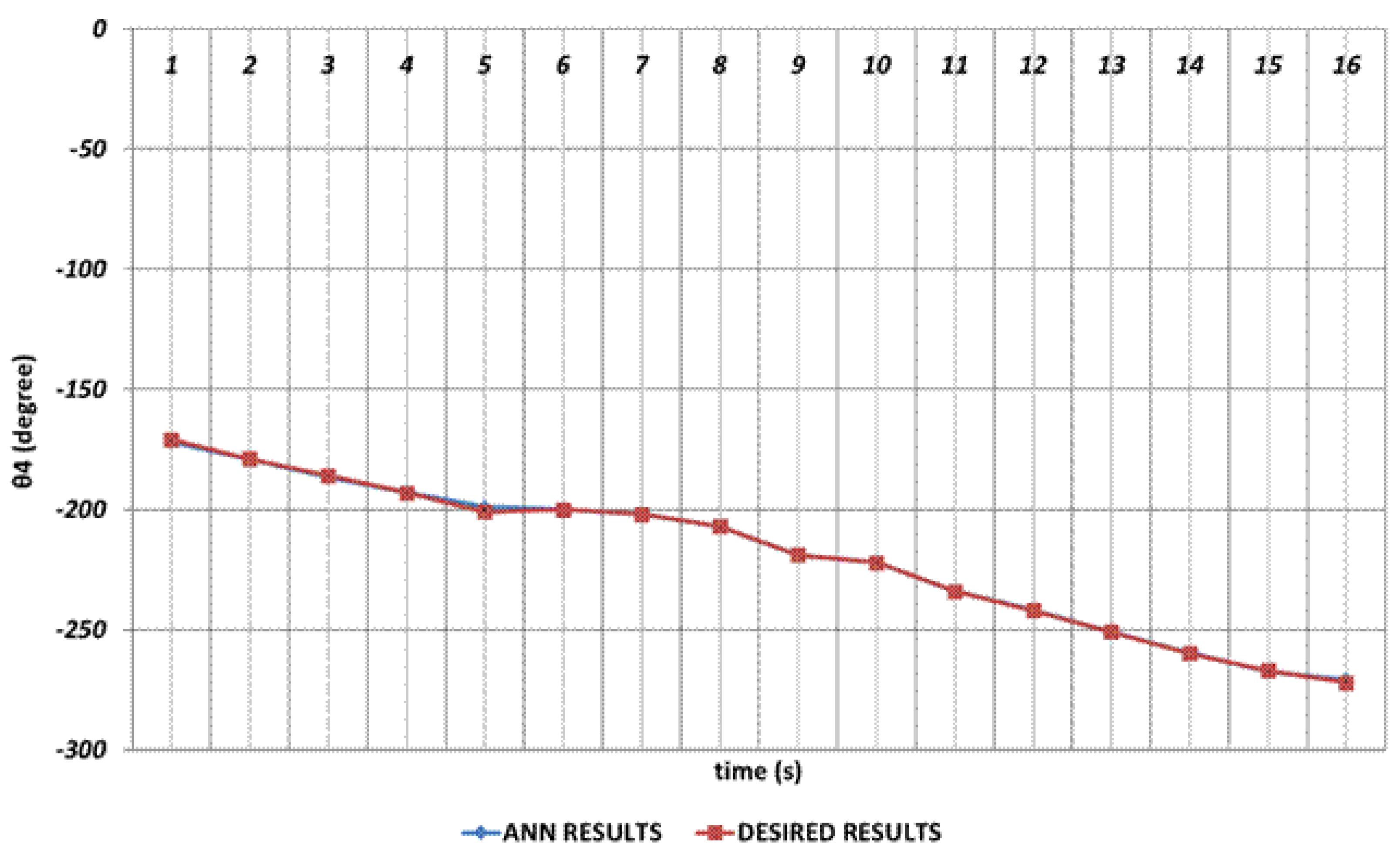
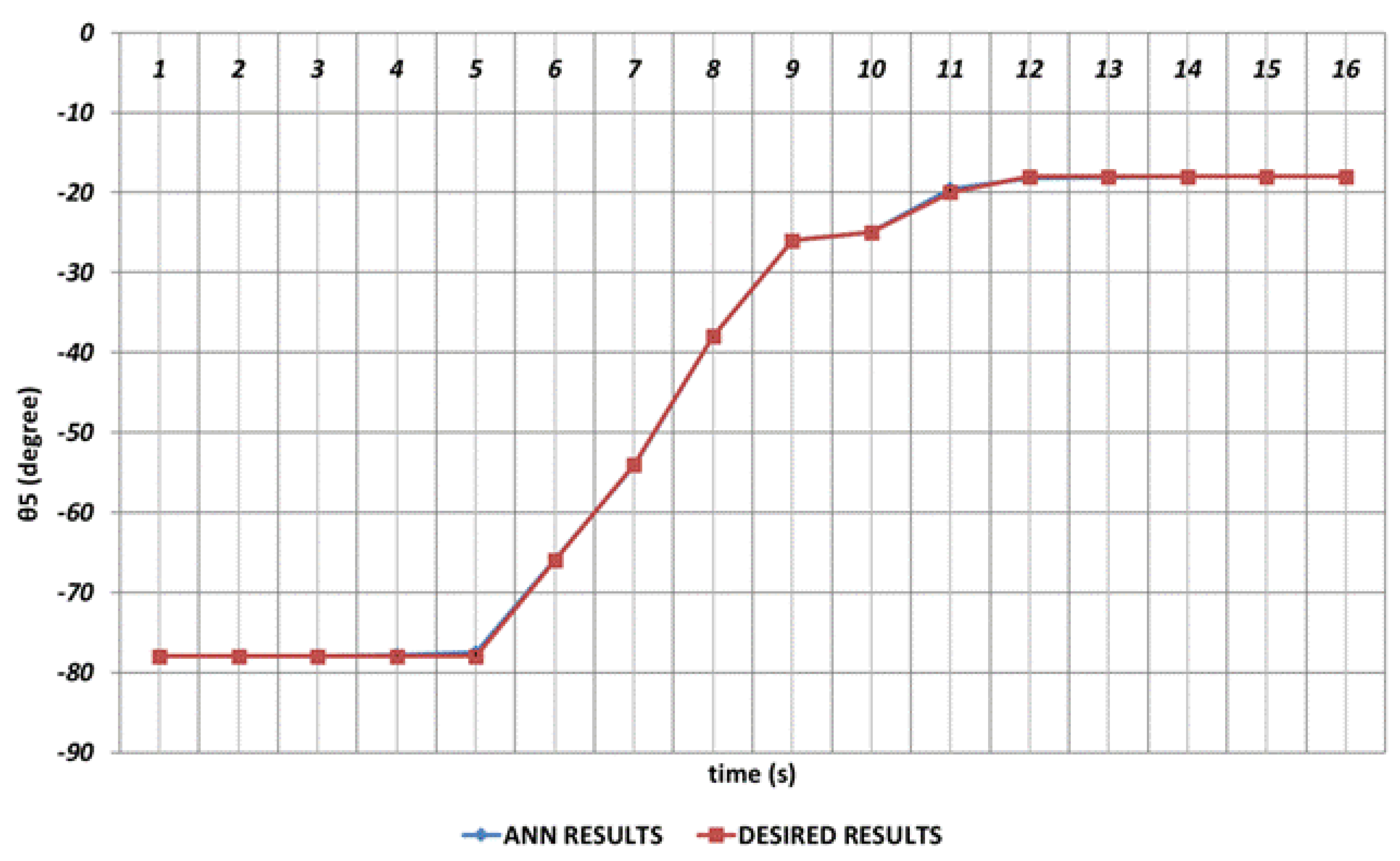
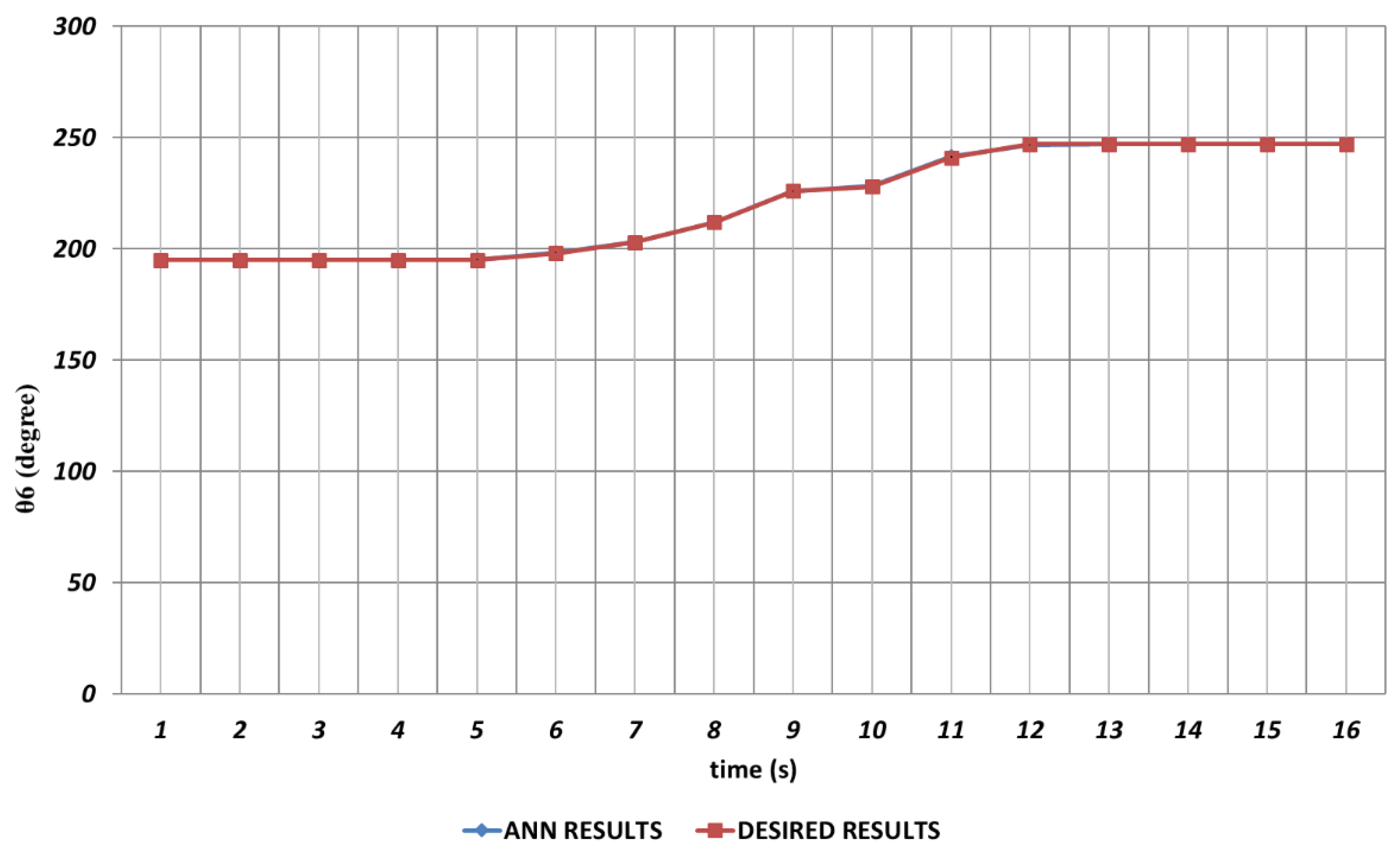
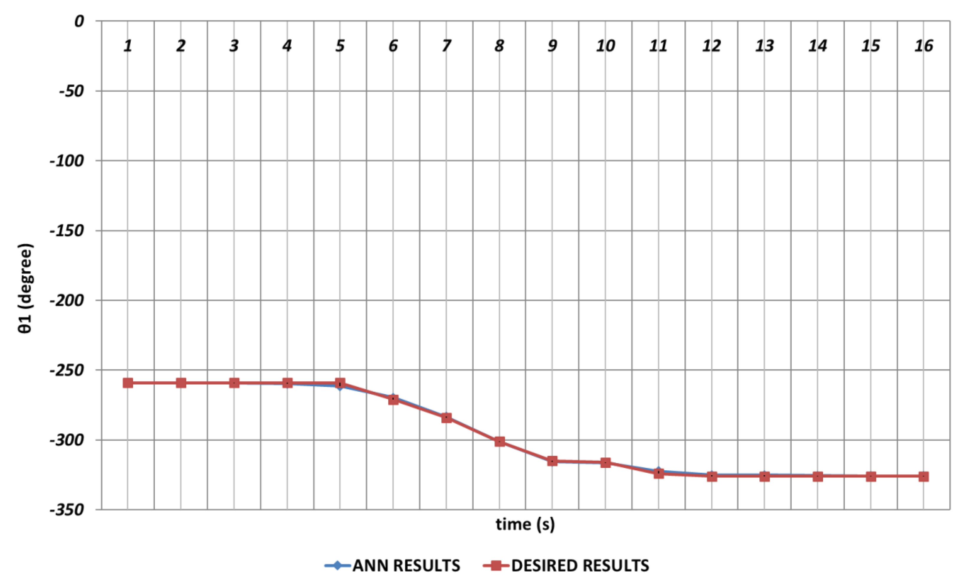
1. Introduction
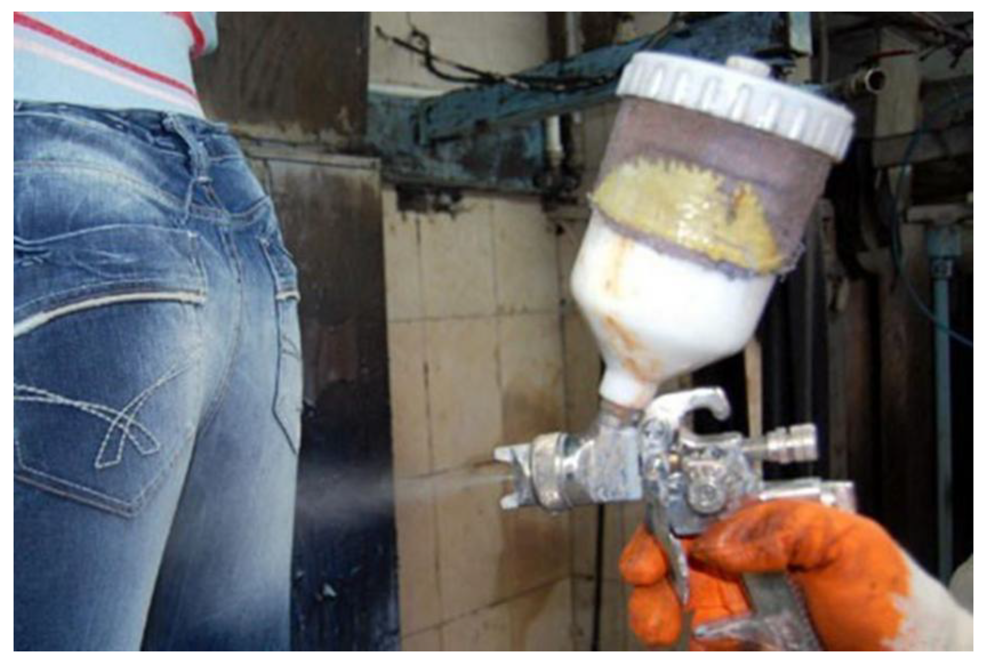
Industrial robots are capable of performing many different processes and operations accurately and do not need complex supporting elements as humans need. Robot manipulators are powerful electromechanical systems which provide effective solutions to the recent industrial applications such as picking, placing, packing, painting and welding. Especially, robot manipultors with multi-DOF are widely used at all stages of production processes such as automation systems due to their ability of performing industrial operations effectively without the need of humans. In addition, significant advantages in terms of occupational health and safety have been provided by switching from the operator-assisted production model to robot manipulator-supported structures in processes involving chemicals and carcinogens.
One of the most important problems encountered in robot manipulator systems is the ability to achieve high-accuracy positioning even large disturbances such as mechanical friction of the mechanical parts, ambient ventilation and mechanical strength misalignment. In this study, ANN-based detailed trajectory analyzes were carried out to enable the robot manipulator end processor to monitor the full trajectory with the highest accuracy during the denim fabric grinding process.
In the literature, there are several studies including different application areas of robot manipulator systems. Saad et al. have been developed an ANN based adaptive controller for robot manipulator applications in [
1]. A geometric algorithm for fixed directional working area calculation in 6-PRRS structured robot manipulators was proposed by Boney and Ryu and its applications were analyzed [
2]. In study conducted by Bonev et al. [
3] on the kinematics of parallel robot manipulators with linear sensors and optimal positioning, a closed-form solution approach was developed. Detailed researches on the singularities of 3-DOF parallel robot manipulator mechanisms were carried out by Boney and his research group [
4]. Tombul and Sarıtaş presented a detailed research which was conducted on inverse kinematic calculations and trajectory planning for a five-axis Edubot robot [
5]. On the other hand, Khayati et al., carried out analysis on multi-stage position/force control for friction-constrained robotic systems [
6]. Lessard et al. carried out analyzes on static balancing optimization by designing position and force controllers for biomedical applications, especially 3-dimensional ultrasound imaging [
7]. Karahan obtained the robot inertia parameters by performing detailed dynamic model analysis for the Staubli RX-60 robot in his master thesis [
8]. In another study, Janvier et al. performed detailed performance analyzes for medical robotic 3-dimensional ultrasound imaging systems [
9]. A parallel medical robot design and its static balancing optimization were carried out by Lessard et al. for medical robotic applications [
10]. An updated formulation and its related applications improved for a KUKA type industrial robot manipulator were presented by Bigras et al. [
11]. Moreover, Yu et al. proposed a geometric approach for accuracy analysis of 3-DOF planar parallel robots [
12]. Furthermore, accuracy analysis of a 3-DOF planar parallel robot structure was performed by Briot and Bonev [
13]. On the other hand, parallel kinematic analyzes were carried out by Liu et al. on a two-joint robot structure and then detailed analyzes on adaptability, error optimization and size optimization were realized [
14]. Bigras et al. performed detailed mathematical equation analyzes for an industrial robot and applied the results to force control [
15]. Furthermore, autonomous movement capabilities of 3-DOF planar parallel robot structures were investigated in detail and then relevant analysis were carried out by Briot and Boney [
16]. A novel controller structure combining the adaptive neural networks and proportional-integral-derivative (PID) control approach was presented by Perez et al. to optimize the trajectory behaivour of robot manipulators [
17]. An ANN based method which is able to adapt to the characteristics of both known and unknown trajectories of 6-DOF robot manipulators was improved by Tang et al. [
18]. Pham and Wang improved a robust radial basis function neural network (RBFANN) based adaptive control approach to optimize the joint position control and trajectory tracking control of robot manipulators [
19]. An inverse dynamic model estimation approach based on ANNs was proposed by Moldovan et el. in study [
20] to optimize the trajectory performance of a 6-DOF robot manipulator. Mahajan et al. improved an ANN based structure to optimize the trajectory tracking of a 2-DOF robotic arm by using the inverse kinematics equations [
21]. Moreover, Son et al. proposed an adaptive ANN model which was strengthened by differential evolution algorithm in order to optimize the non-linear dynamics of a 5-DOF robot manipulator [
22]. An ANN based control process with optimal number of hidden nodes and less computation was proposed by Liu et al. to overcome the system uncertainities and track the trajectory of robot manipulator with high accuracy [
23]. Truong et al. proposed a novel adaptive tracking ANN with deadzone robust compensator for industrial robot manipulators to achieve the high precision position tracking performance [
24]. On the other hand, Elsisi et al. proposed an ANN based modified adaptive tuning algorithm in order to track the trajectories of robot manipulator arms with high accuracy [
25]. Finally, a multi-objective design mechanism was introduced by Kouritem to determine the optimal material type and optimal physical dimensions of the robot arm to withstand loads at vulnerable locations using stress analysis [
26].
3. Simulation Results
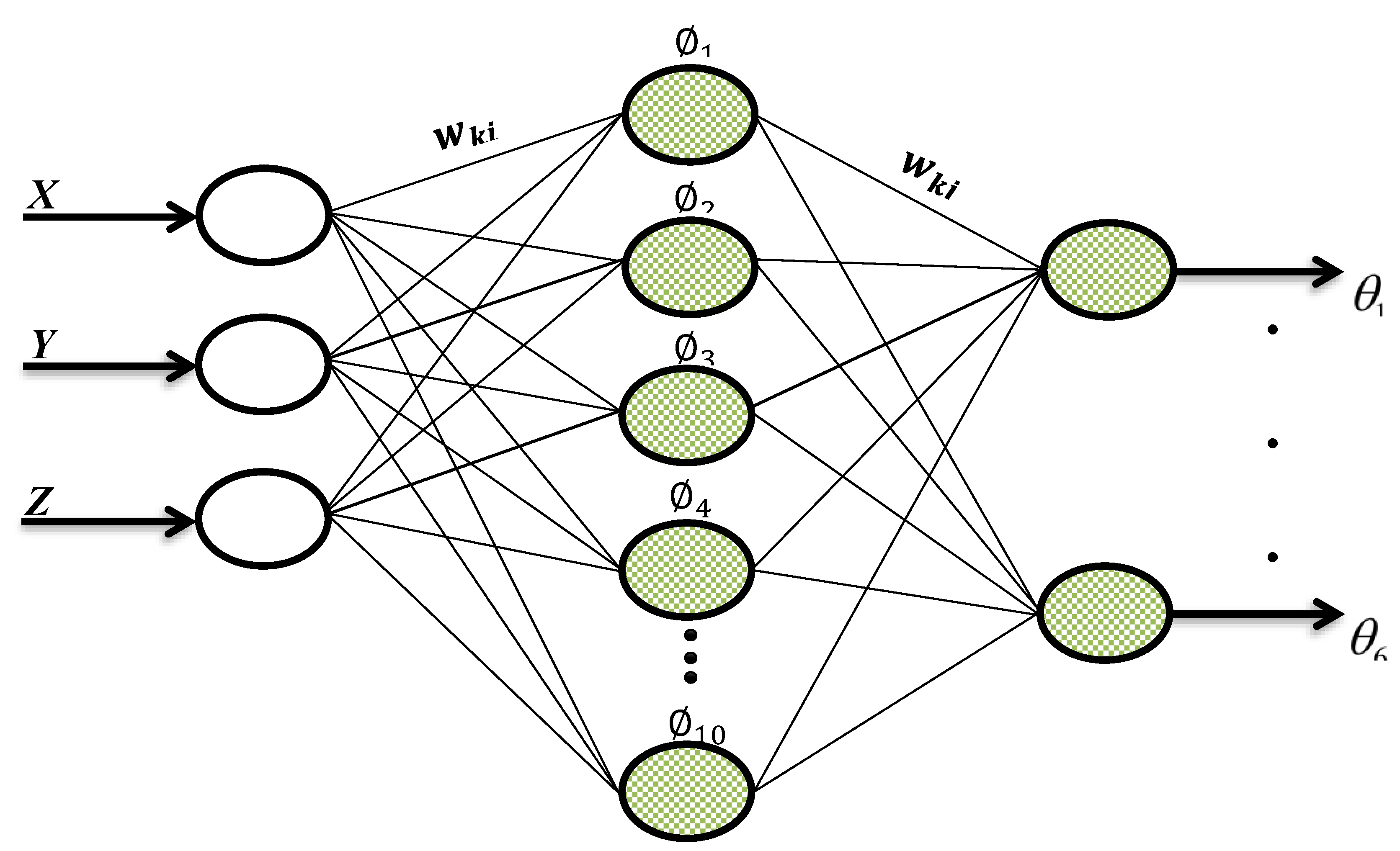
In the simulations carried out the ANN structure consists of 3 input cells (position of the end function - X, Y, Z), 10 hidden layer cells and 6 output layer cells (joint angels - and ) are formed. Furthermore, randomly selected %70 of the entire data set was used for the training of the ANN and the remaining %30 data were used for test phase. In all the simulations the iteration number was taken as 1000000.
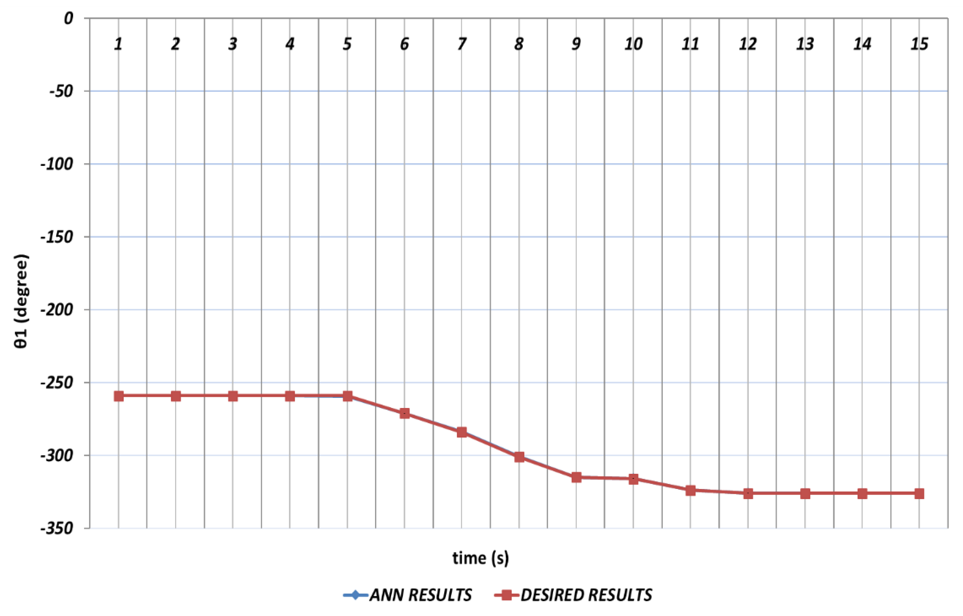
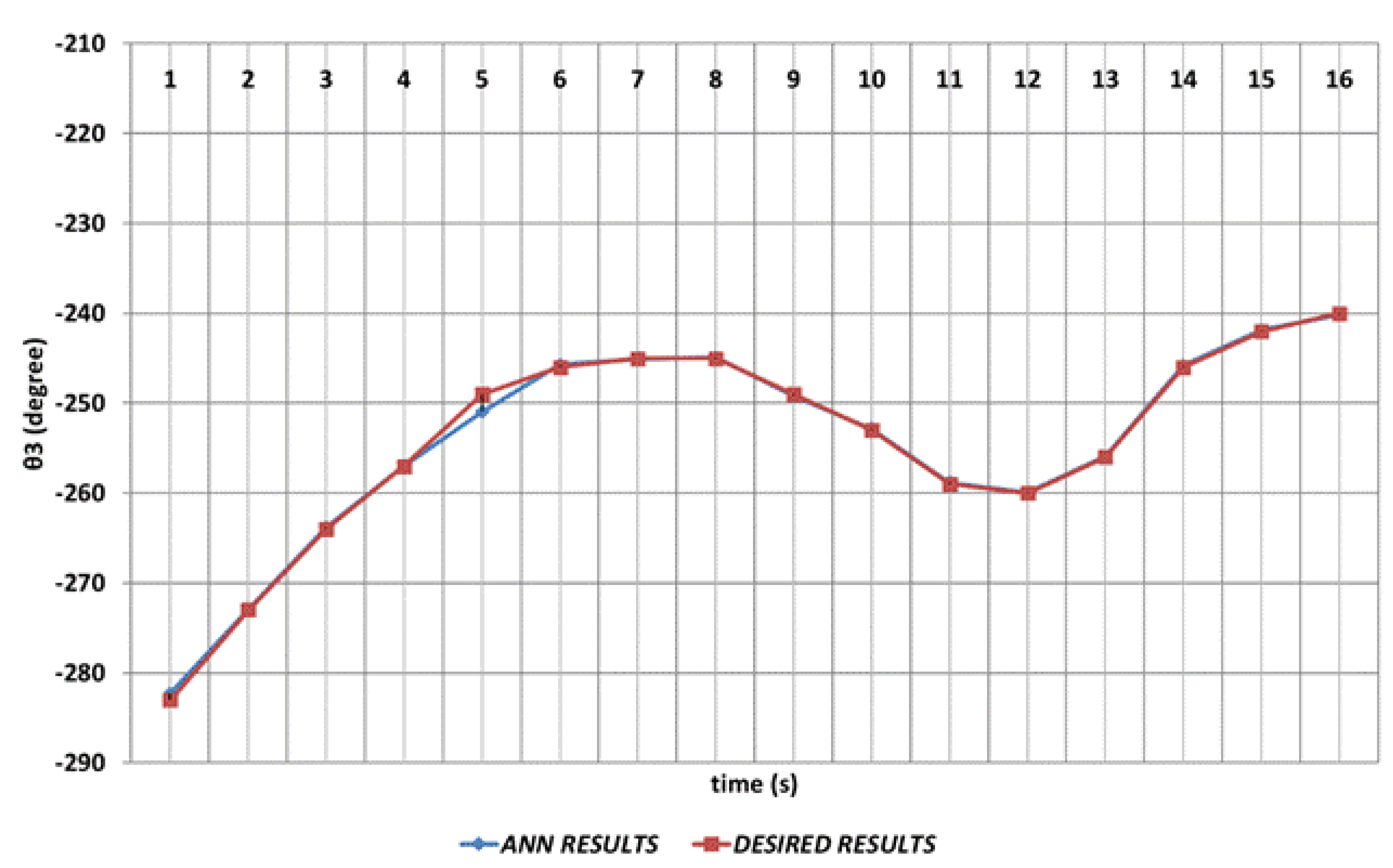
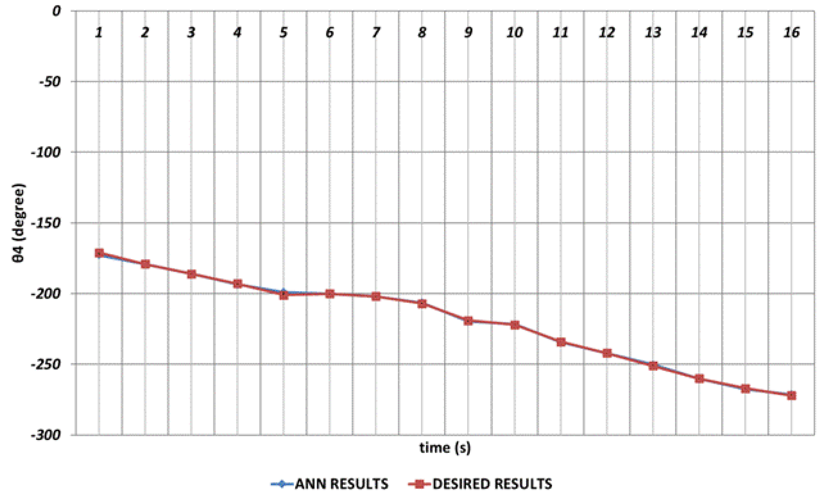
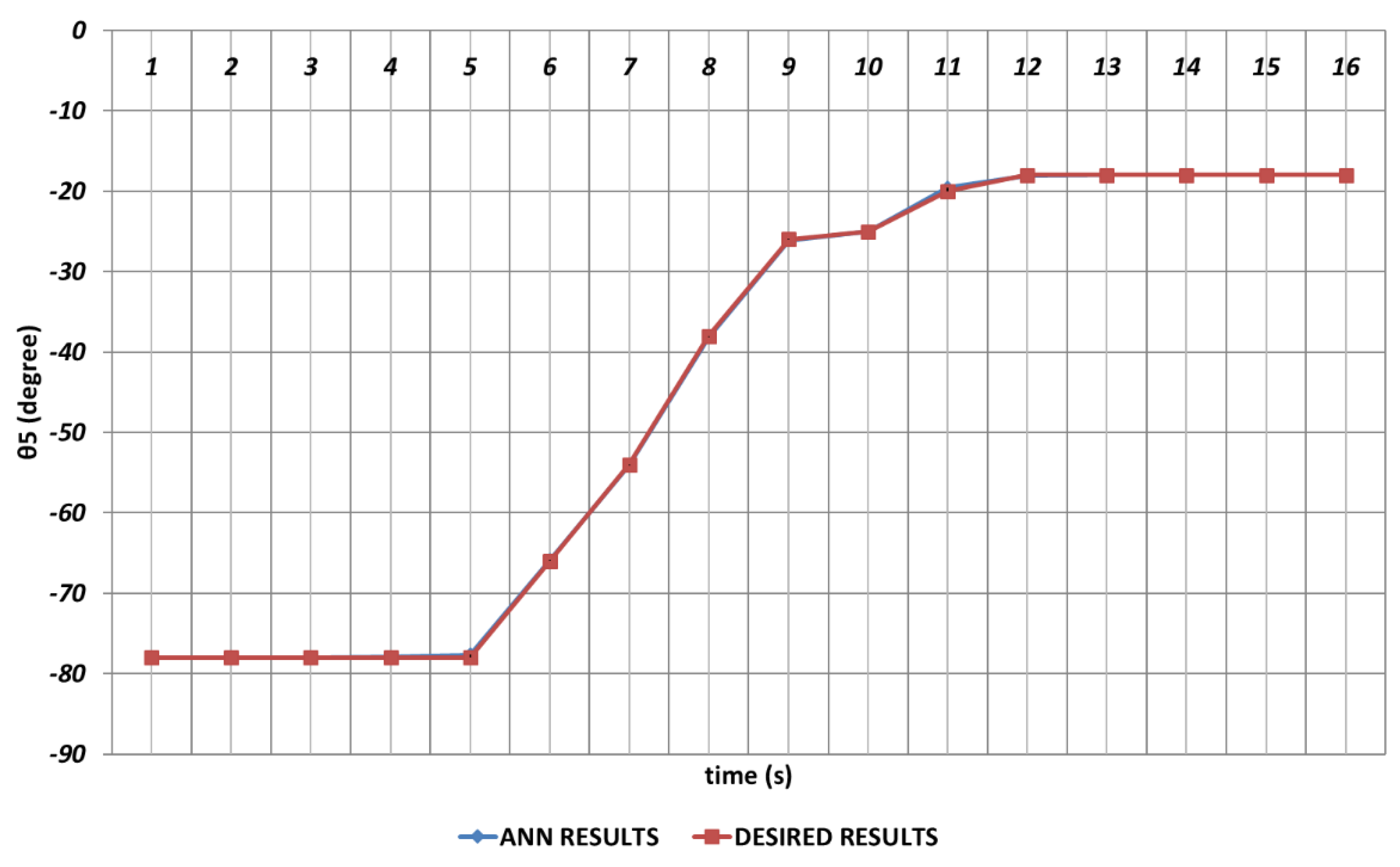
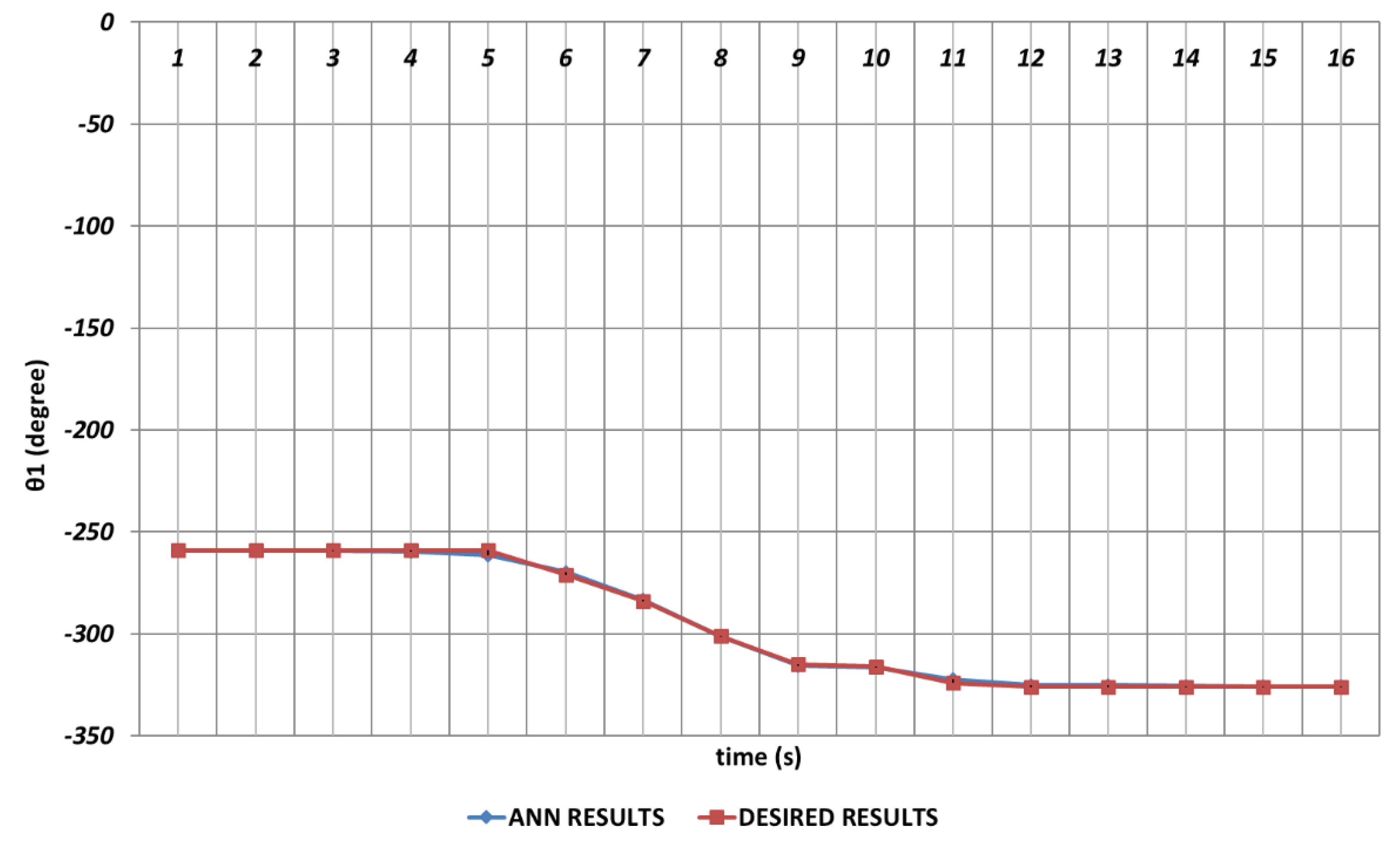
In
Figure 6,
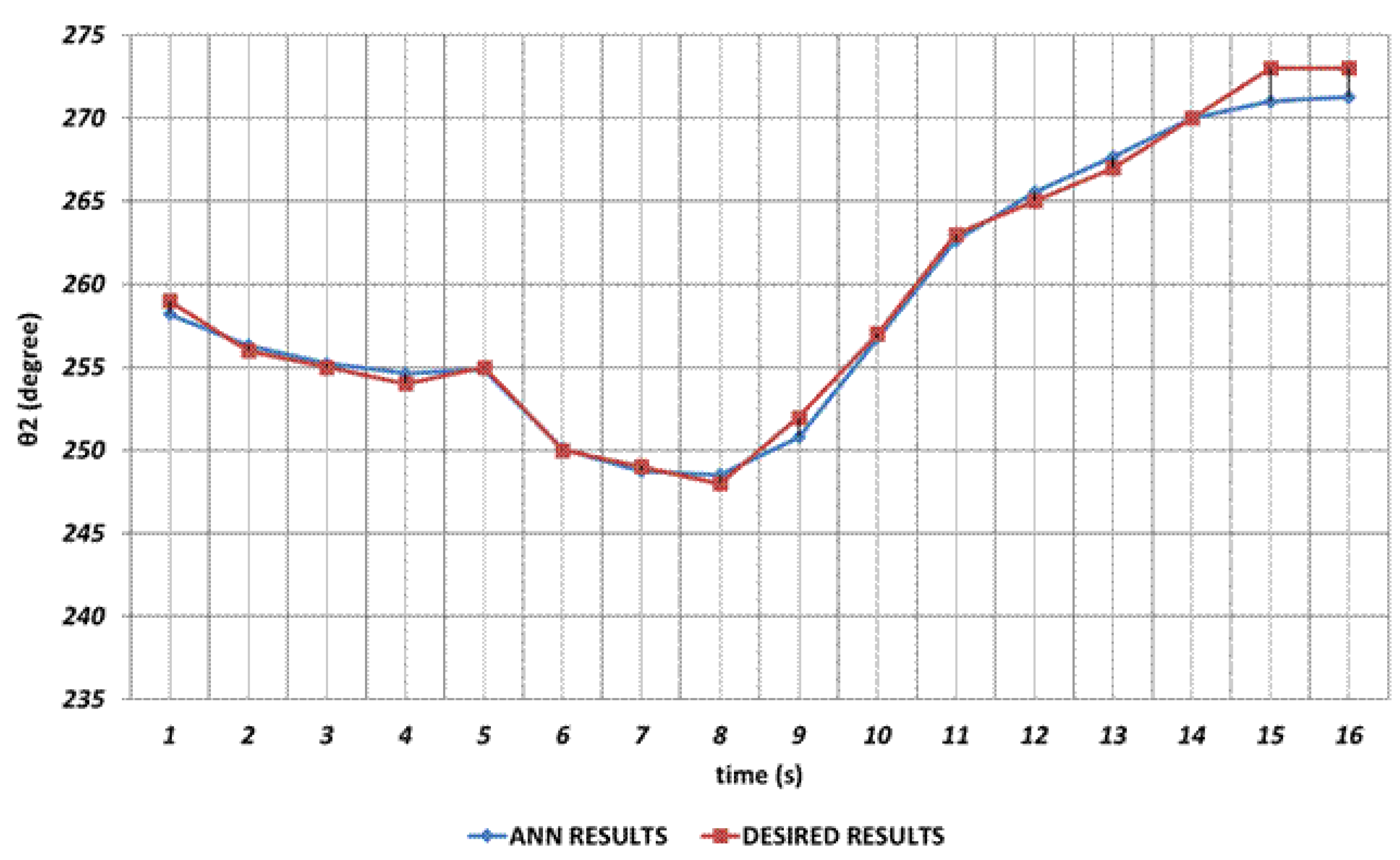
Figure 7,
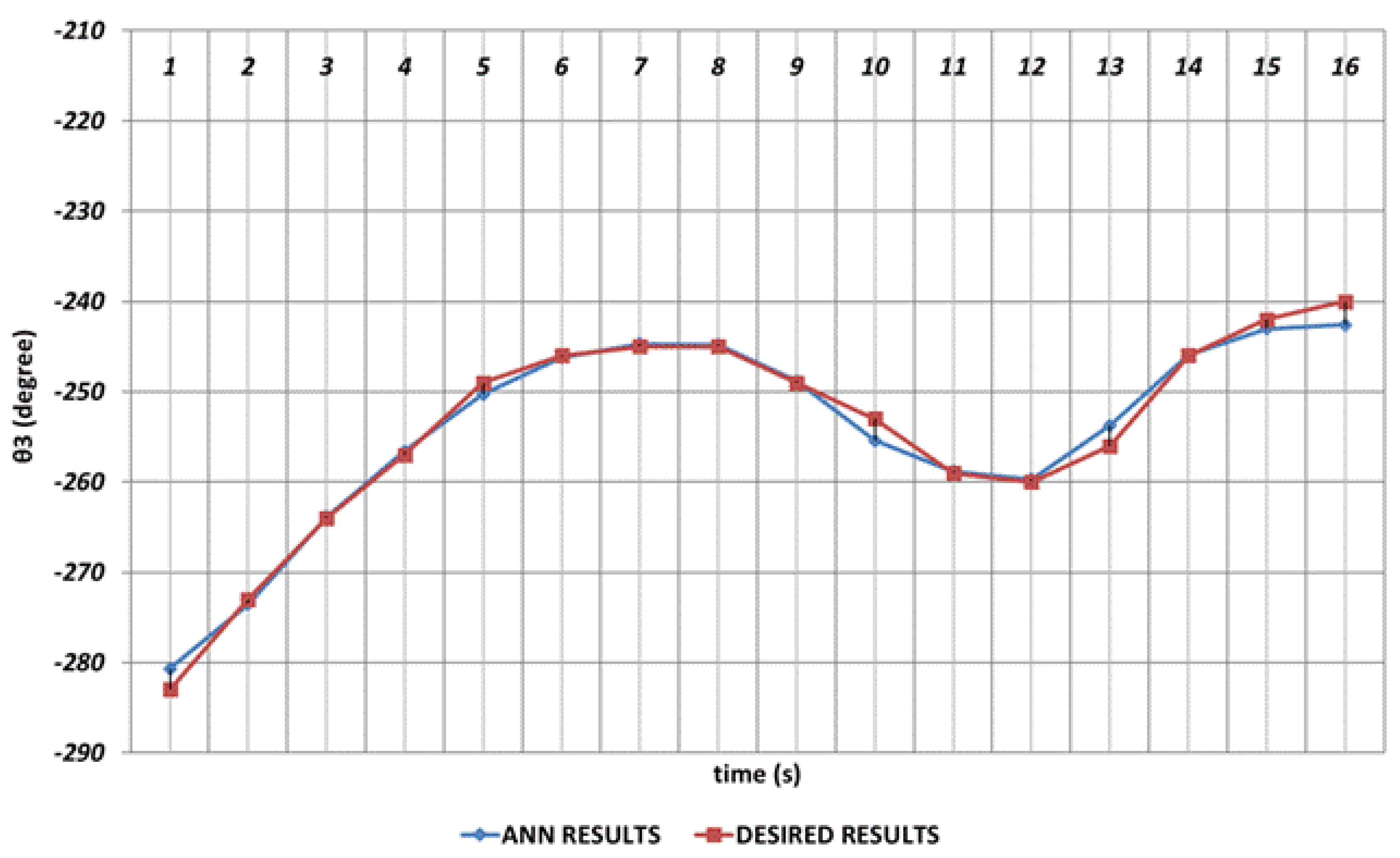
Figure 8,
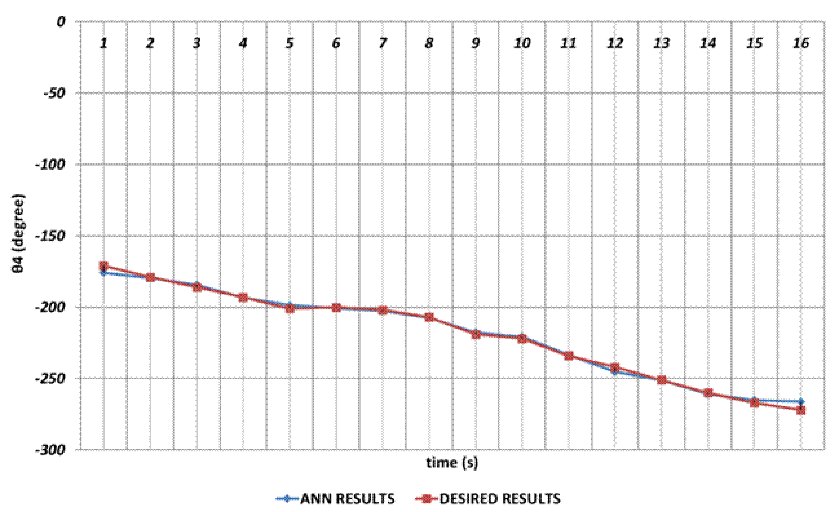
Figure 9,
Figure 10 and
Figure 11, DBD learning algorithm based simulations results are presented. As seen from the
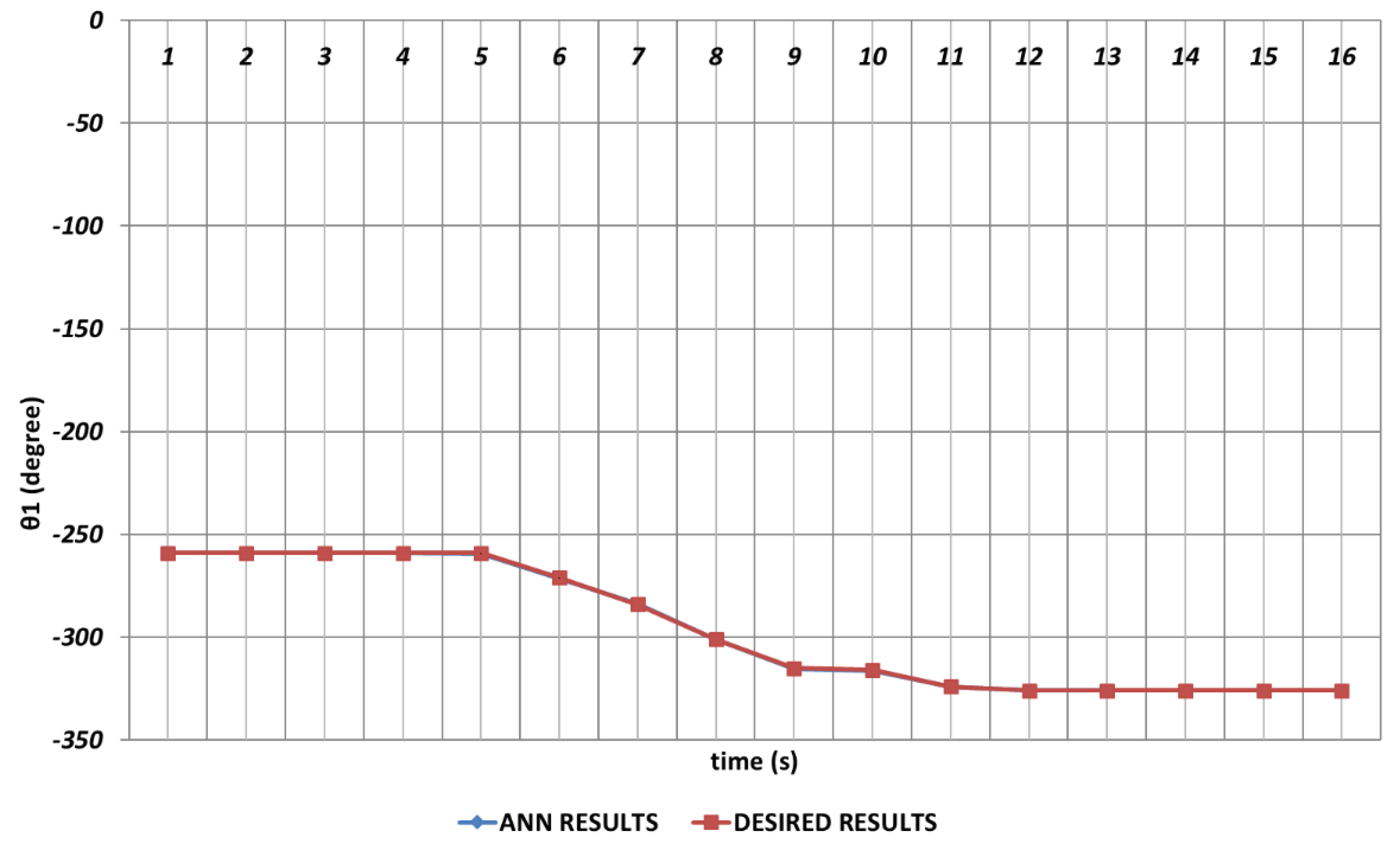
Figure 6, which represents the modelling performance for
, DBD algorithm is able to predict the theoretical data with high accuracy. Although there are instantaneous angular changes at the 5
th and 9
th seconds, the DBD can follow these changes successfully.
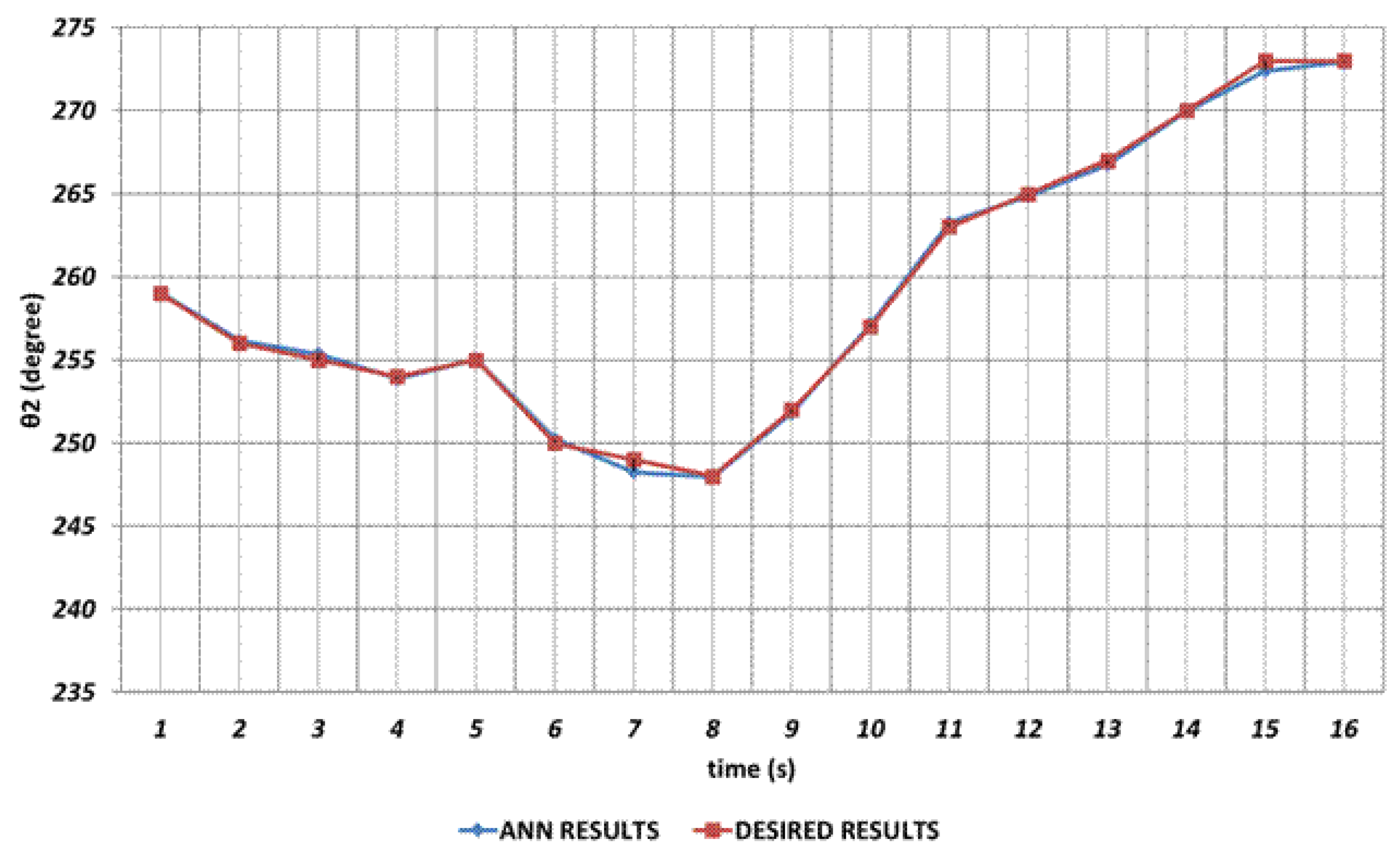
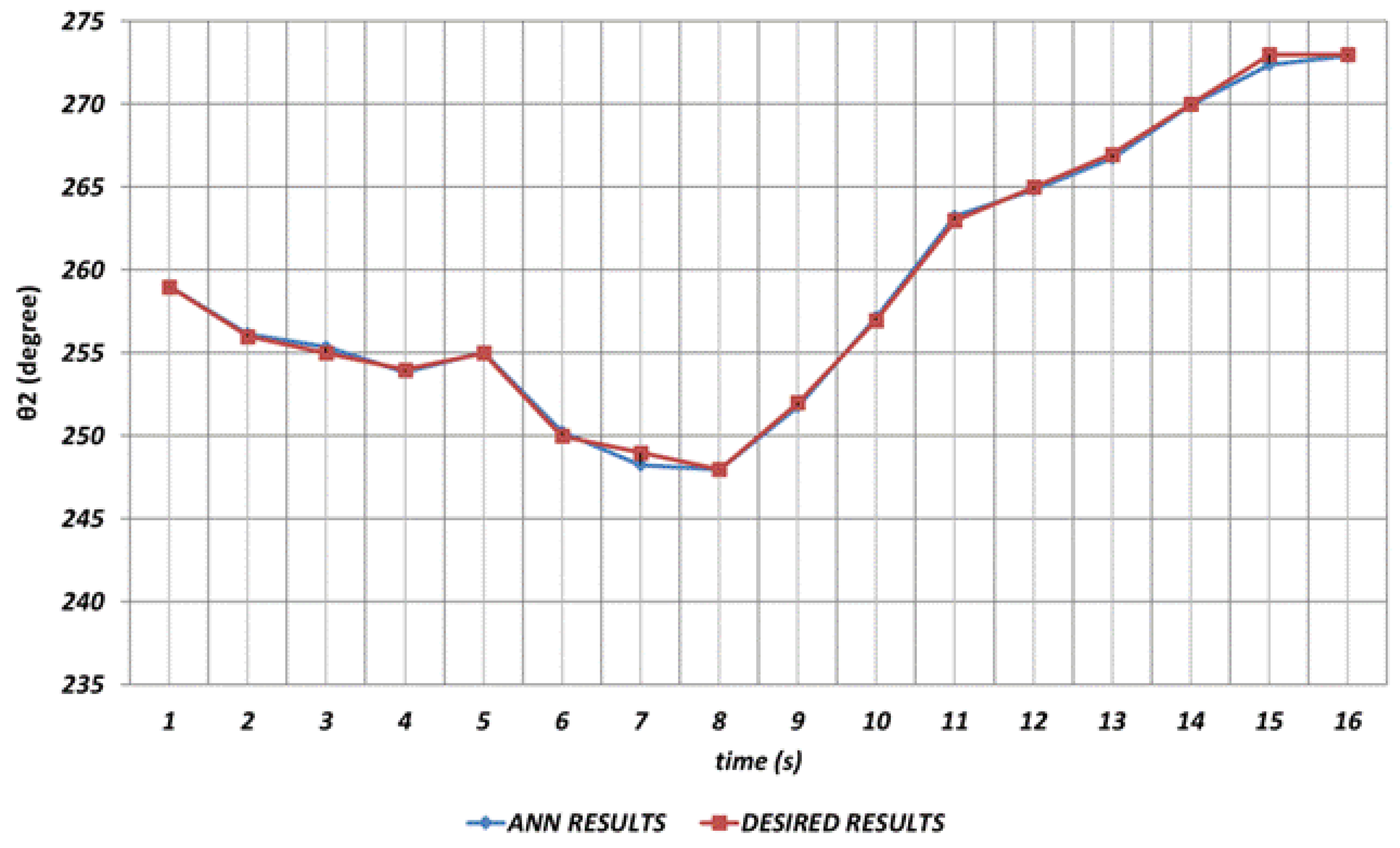
Figure 7 shows the DBD based prediction result for
. Since it is used as the shoulder angle, it is seen that there are significant prediction errors in the intervals of 2
nd and 4
th seconds, 6
th and 8
th seconds and similarly 14
th and 16
th seconds. Namely, DBD based estimation seems a bit insufficient in predicting instantaneous changes in the time intervals mentioned. This situation shows that an unexpected position difference will occur in serial chemical application between the fabric where the chemical will be sprayed and the ideal position.
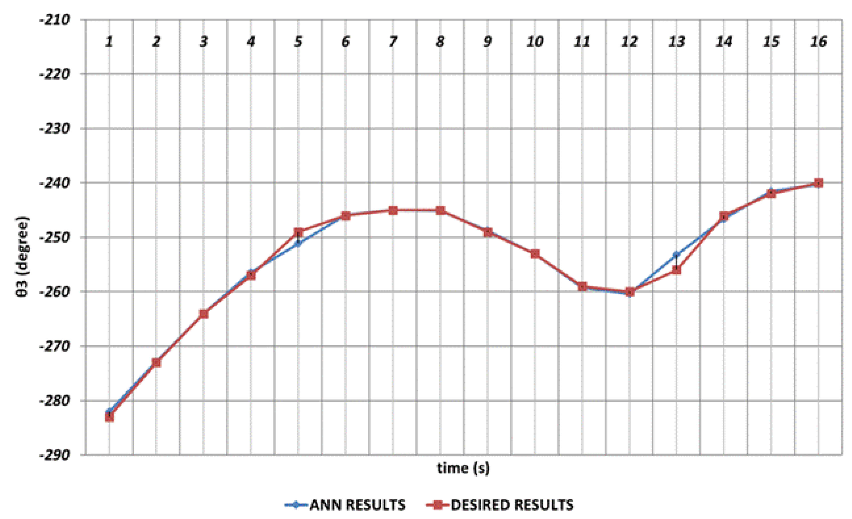
DBD based prediction results of the
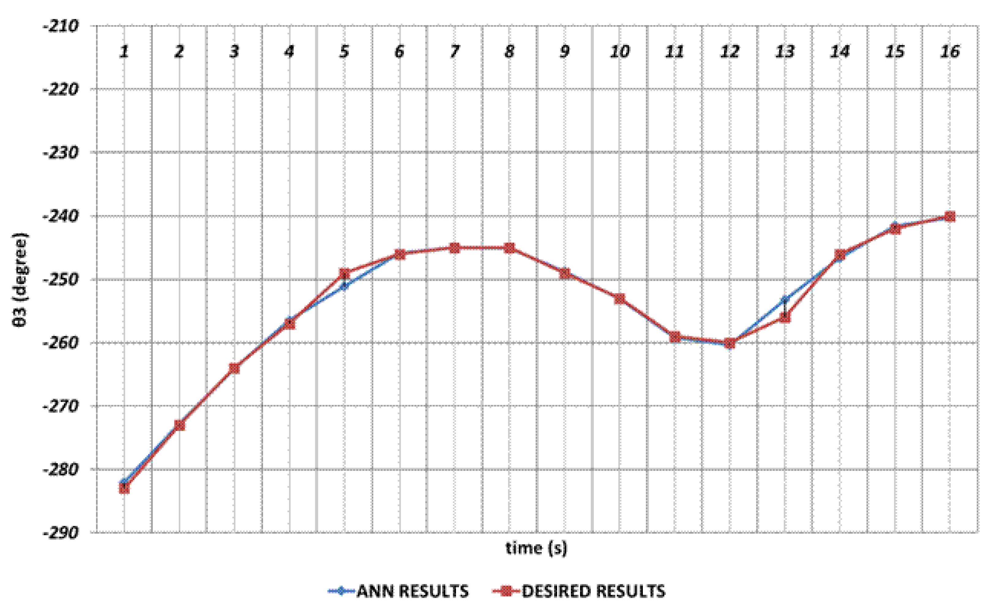
, which performs the elbow function in the human structure, is demonstrated in
Figure 8. Since the shoulder angle appearing after the angular change is used as the next period angle at the same time, instantaneous changes in the time intervals of 1
st and 2
nd seconds and also 4
th and 6
th seconds observed. It can be concluded that significant spray errors will occur will be observed, especially in the time interval of 4
th and 6
th seconds, in serial chemical applications. On the other hand, despite the errors that occur during instantaneous angular changes, the prediction performance seems successful outside of these two time intervals.
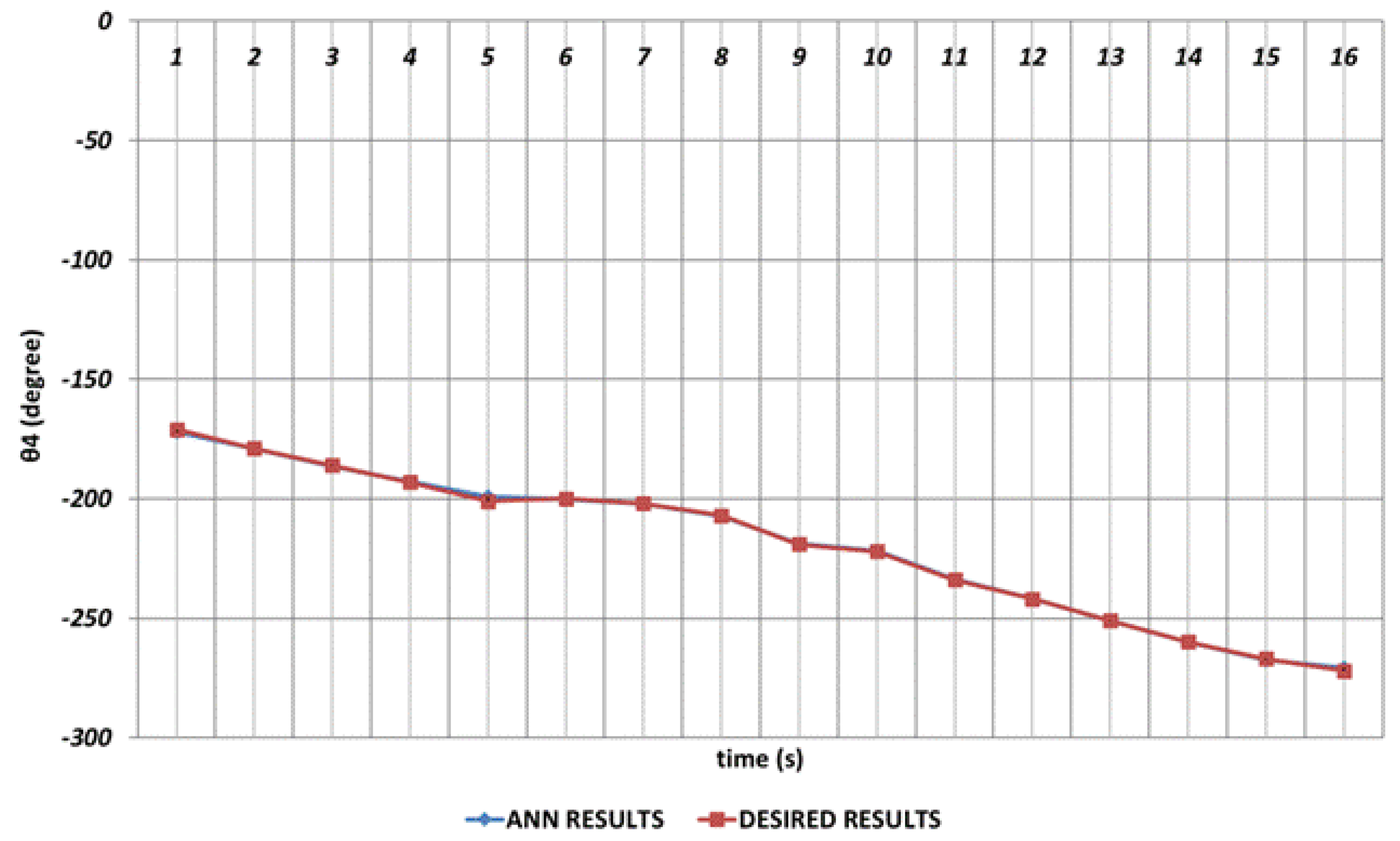
The joint angle corresponds to the rotation angle of the robot gripper. When the DBD based prediction results anlayzed, it can be emphasized that the theoretical data can be predicted with high accuracy even in the intervals of 4th and 6th seconds and 8th and 10th seconds at which instantaneous angular changes appeared.
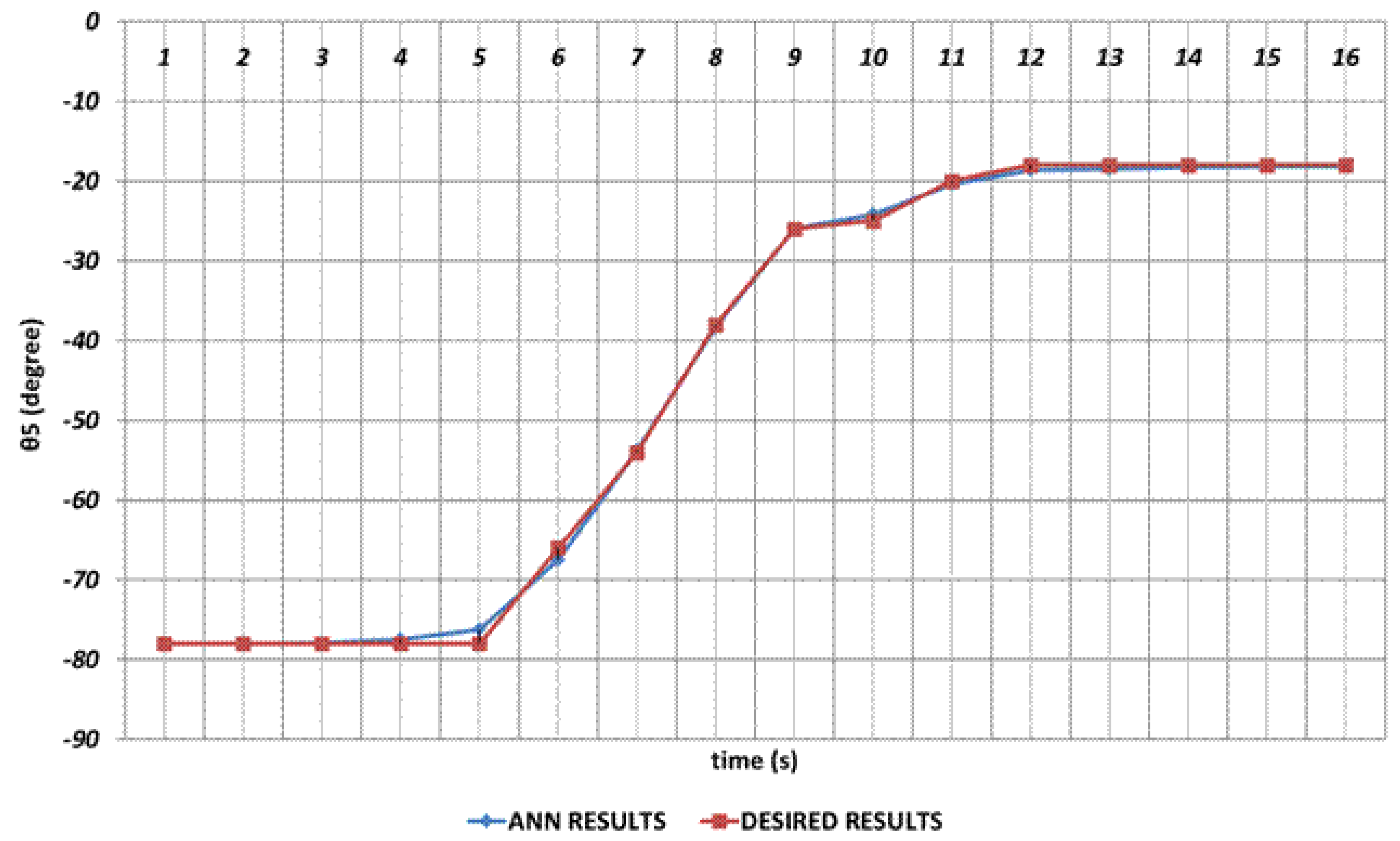
Especially the fifth joint angle has an important role in positioning structure and rotation angle and even small prediction errors for
are not acceptable. Firstly, instantaneous angular changes occur in the intervals of 4
th and 5
th seconds and similarly in the 10
th and 12
th seconds, as seen in
Figure 10. As a result of these instantaneous angular changes, it is seen that deviations with too small magnitudes are occurring in the DBD based prediction results. When the prediction performance is evaluated in a general manner, it can be expressed that DBD can successfully predict the theoretical data for
.
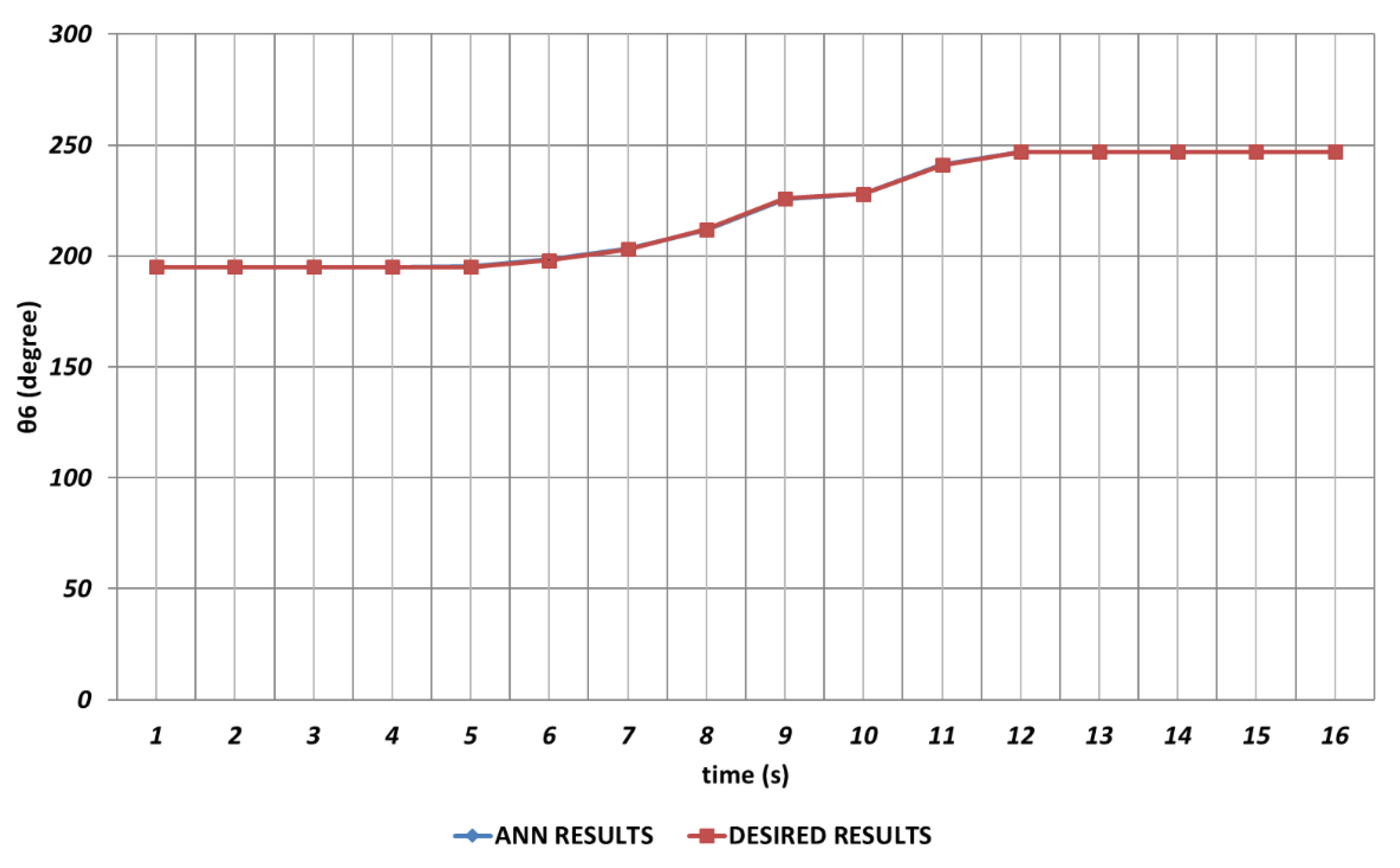
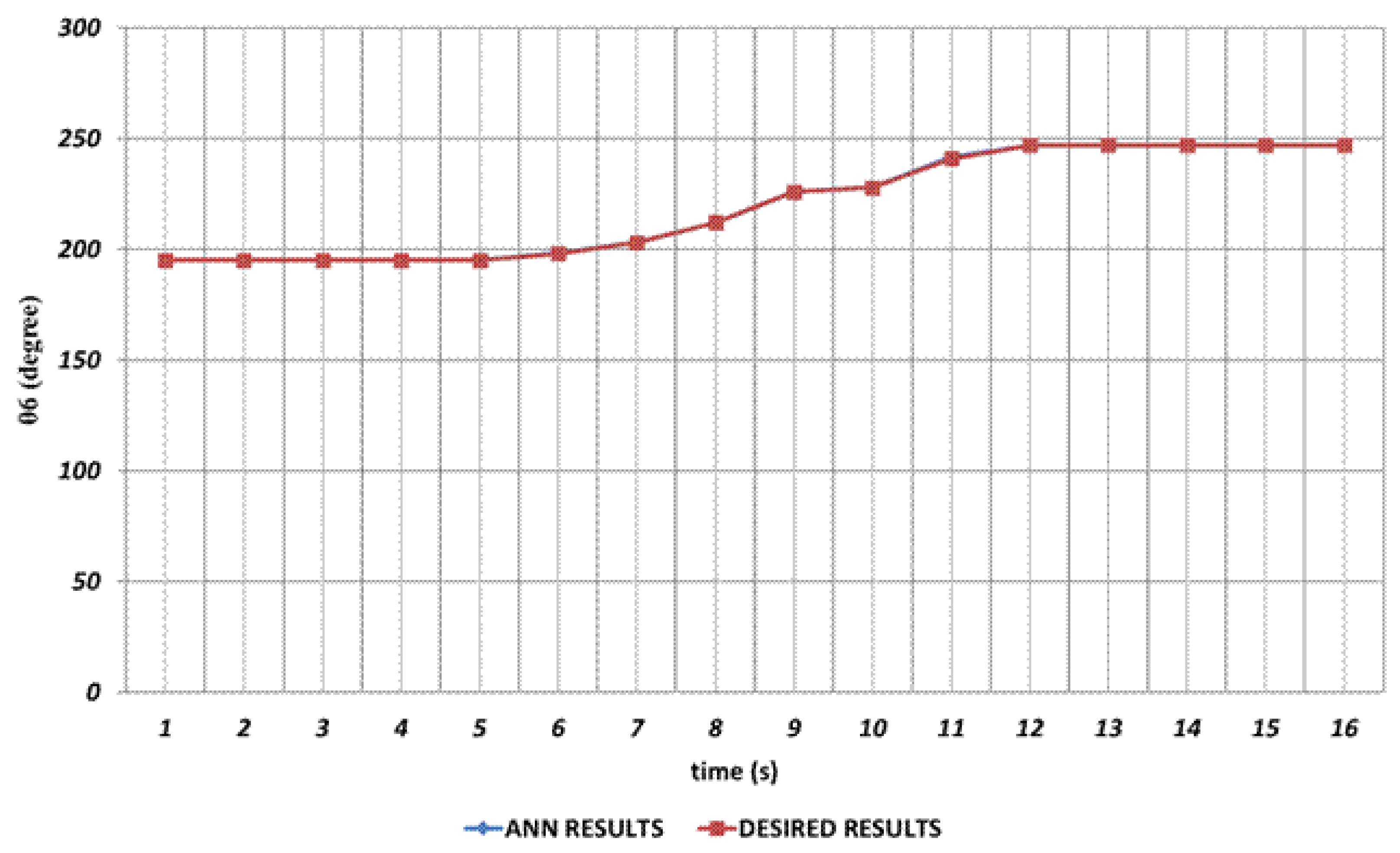
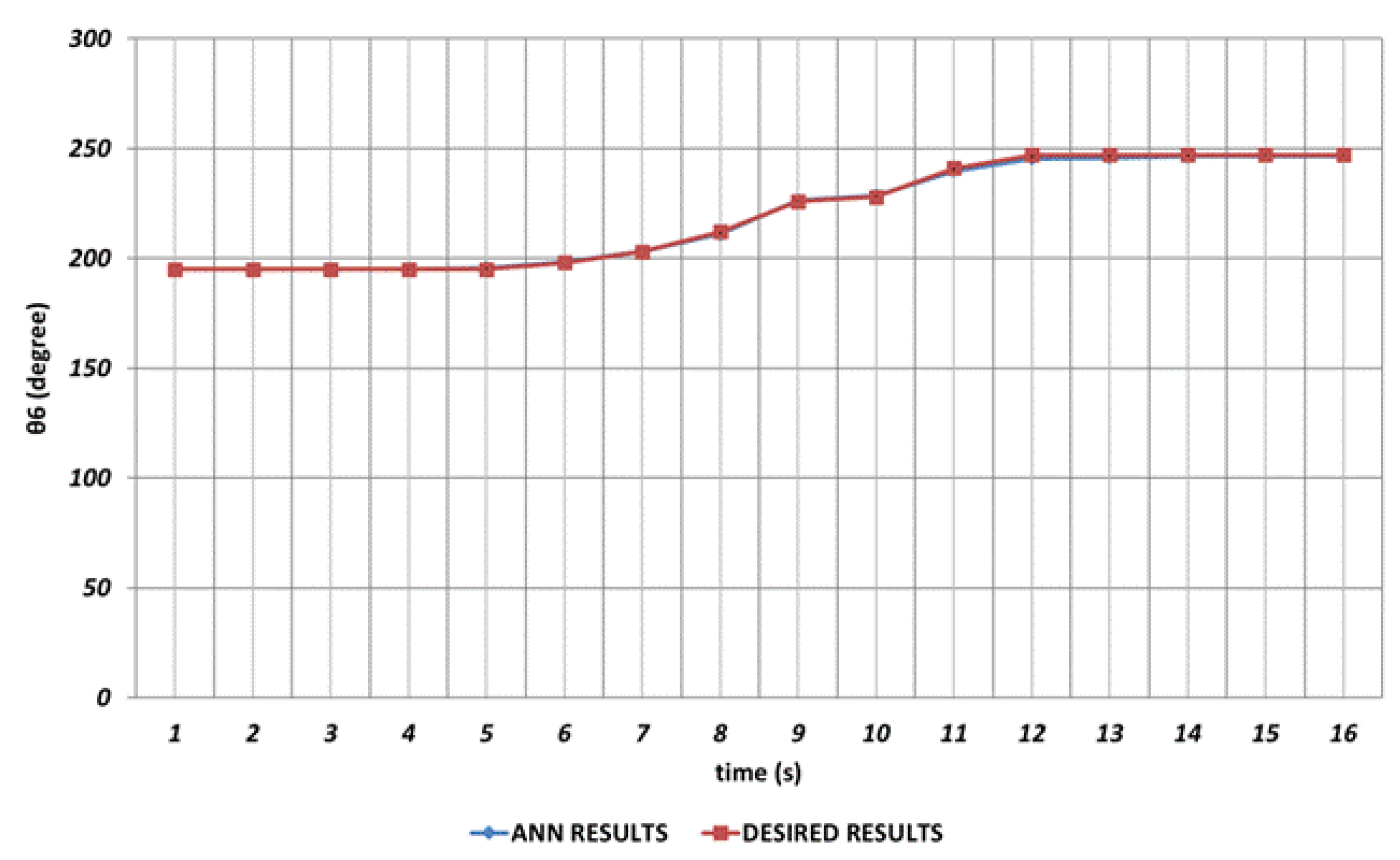
Figure 11 shows the prediction results obtained for
which is the last rotation angle of the robot manipulator. It is seen that small prediction errors are almost non-existent for the sixth joint angle. The reason of this can be expressed as no instantaneous angular changes are occurring during the entire time interval.
The analysis results obtained for the OBP learning algorithm are given in
Figure 12,
Figure 13,
Figure 14,
Figure 15,
Figure 16 and
Figure 17. The prediction performance for the
joint angel is presented in
Figure 12. From the figure, it is seen that OBP is able to produce superior prediction result for the first joint angle which is the body rotation angular of the robot manipulator. In other words, no instantaneous angular changes are occurring and the OBP based results converges to the theoretical results with high accuracy during the entire time interval.
In
Figure 13, the prediction performance of the OBP learning algorithm is shown for the
joint angle which corresponds to the corresponds to the shoulder angle. It is seen that there are significant prediction errors in the time intervals of 2
nd and 4
th seconds, 6
th and 8
th seconds and 11
th and 16
th seconds due to the instantaneous angular changes. These angular differences will cause the chemical spraying process to be carried out with incorrect angle values.
Figure 14 demonstrates the OBP based prediction results obtained for
which is the third joint angle of the robot manipulator. Since the shoulder angle obtained after the angular change is used as the next period angle at the same time, it is observed that significant deviations from the theoretical data are appeared in the time intervals of 1
st and 2
nd seconds, 4
th and 6
th seconds and also 11
th and 16
th seconds. As a result, it can be emphasized that the prediction performance for the third joint angle seems insufficient when the OBP learning algorithm used. In contrast, OBP is able to provide better prediction performances outside of the time intervals that include instantaneous angular changes.
In
Figure 15, the simulation results produced by OBP in prediction of
joint angle are presented. From the results, it can be expressed that the rotation angle of the robot gripper can successfully be predicted with high accuracy via OBP learning algorithm. However, although instantaneous angular changes have no significant effect, it is seen that prediction errors are occurring between the theoretical and ANN approach at certain rates in the time intervals of 4
th and 6
th seconds and 14
th and 16
th seconds.
joint angle is extremely important for the positioning of the end effector used in the chemical spray system. Due to its critical role in optimizing the positioning structure of the entire system, even small prediction errors are not acceptable for this angle as mentioned before. As seen from the prediction results given in
Figure 16, deviations with too small magnitudes occurring especially in the time intervals of 3
rd and 6
th seconds and 10
th and 13
th seconds
As seen from the
Figure 17, which represents the OBP based prediction results obtained for
, an excellent prediction performance can be provided. The limited number of instantaneous position changes in the theoretical data ensures an effective prediction process during the entire time interval.
The prediction performance of QBP learning algorithm in terms of the joint angles are represented in
Figure 18,
Figure 19,
Figure 20,
Figure 21,
Figure 22 and
Figure 23.
Figure 18 proves that QBP is able to provide an excellent prediction performance for
during the entire time interval, including instantaneous angular changes.
QBP based prediction results for the robot manipulator shoulder angle
is shown in
Figure 19. As can be seen from the figure, there are significant prediction errors especially in the time intervals of 2
nd and 4
th seconds, 6
th and 8
th seconds and 14
th and 16
th seconds due to the effect of instantaneous angular changes. In other words, the prediction results for
should not be used directly in serial chemical applications.
Figure 20 demonstrates the QBP based prediction result for the
joint angle which simulates the elbow function of humans. Due to the instantaneous angular changes in the time intervals of 1
st and 2
nd seconds, 4
th and 6
th seconds and 11
th and 14
th seconds, the therotical data cannot be predicted successfully. As a result, it can be emphasized that the prediction for the third joint angle is not very effective and the performance of the QBP seems insufficient at the relevant time intervals.
In
Figure 21, the QBP prediction results obtained for the
joint angle are given. In general, it can be said that QBP can successfully converge to the theoretical data except the time intervals of 4
th and 6
th seconds and 14
th and 16
th seconds. On the other hand, it can also be stated that the deviations from the theoretical data are occurring with too small magnitudes in the relevant time intervals.
Due to its importance mentioned before, the prediction of the
joint angle with high accuracy is crucial.
Figure 22 represents the prediction performance of the QBP learning algorithm. Due to the effect of instantaneous angular changes, it is seen that prediction errors with small magnitudes are occurring between the theoretical data and QBP approach in the time intervals of 4
th and 6
th seconds and 10
th and 12
th seconds. When the prediction performance is evaluated in a general manner, it can be expressed that QBP can successfully predict the theoretical data for
.
When the proposed QBP based approach applied to the prediction of sixth joint angel, it is seen that the
can successfully be predicted. As seen from the
Figure 23, QBP is able to produce a prediction performance that almost overlapped with the theoretical data during the entire time interval. The reason for this situation may be expressed as the lack of instantaneous angular changes or their occurrence with too small magnitudes.
Figure 24,
Figure 25,
Figure 26,
Figure 27,
Figure 28 and
Figure 29 represent the analysis results obtained by using RBP learning algorithm. As seen from the
Figure 24, which shows the modelling performance for
, RBP is able to predict the theoretical data with high accuracy. Although there are instantaneous angular changes at the 4
th and 6
th seconds, the RBP can also converge to these changes successfully.
Figure 25 demonstrates the RBP based prediction result for
. As seen from the figure, the deviations with high amplitudes from the theoretical data are occurring during the entire time interval.
corresponds to the shoulder angle of the robot manipulator and it is seen that the prediction performance of the RBP in terms of
decreases significiantly as a result of the instantaneous angular changes. In other words, it will be inevitable that the lack of high prediction performance for the second joint angle will cause significant errors in chemical applications in the production process.
In
Figure 26, the prediction results obtained for
by using RBP based ANN are shown. As in the prediction process of the second joint angle, the RBP produces worse prediction results during the entire time interval and also cannot converge to the theoretical data of the
joint angle enough. Namely, basic RBP learning algorithm seems insufficient in predicting the theoretical data of the third joint angle.
In predicting of
joint angle, RBP learning algorithm cannot provide a completely adequate performance as shown in
Figure 27. Especially, deviations having high magnitudes from the theoretical data are occurring in the time intervals of 1
st and 2
nd seconds, 11
th and 13
th seconds and 15
th and 16
th seconds due to the instantaneous angular changes. In addition, deviations having small magnitudes are also observed in the time intervals of 4
th and 7
th seconds and 8
th and 11
th seconds
RBP based prediction performance for the
joint angle is given in
Figure 28. Due to the effect of instantaneous angular changes, it is seen that prediction errors are occurring at unacceptable rates between the theoretical and RBP approaches in the time intervals of 3
rd and 7
th seconds and 9
th and 16
th seconds.
The the prediction results obtained for
are shown in
Figure 29. From the figure, it can be seen that RBP learning algorithm is able to provide an effective prediction performance during the entire time interval except the 11
th and 14
th seconds. It can also be concluded that the lack of instantaneous angular changes or their occurrence with too small magnitudes results in an effective prediction performance.
In order to present a more detailed analysis, in addition to the 3-10-6 ANN network structure including 10 nonlinear cells in the hidden layer, the performance of the 3-5-6 network structure which includes 5 nonlinear cells in its hidden layer is also analyzed. The results obtained are presented in
Table 3. From the results, it is seen that that the network structure including 5 nonlinear cells in its hidden layer can provide a faster learning effect. However, it is also seen that as the number of nonlinear cells in the hidden layer decreases, the error performance and therefore the prediction performance decrease. When the results are evaluated in general, it can be expressed that the QBP produces the best prediction results fot the 3-10-6 network structure while the DBD produces the best prediction results for 3-5-6 network structure.
The statistical performances of the improved ANN network structures are another important performance metric. In this study, the R
2 statistical analysis approach was applied to test the reliability and stability of the results obtained. In Equation 8 given for R
2,
can be defined as the ideal values of the joint angels,
represents the joint angel values obtained from the regression equation and finally
is the mean value of the ideal joint angels. The value of the R
2 parameter changes in the interval of [0,1], The R
2 values close to 1 prove the effectiveness of the model. From the
Table 4 which represents the statistical performances of each algorithm, it can be concluded that all the learning algorithms are able to provide statistically superior performance. In other words, each learning algorithm exhibits stable behavior by converging to approximately the same results at each run.
Figure 1.
Classical human based chemical spraying process on denim textile.
Figure 1.
Classical human based chemical spraying process on denim textile.
Figure 2.
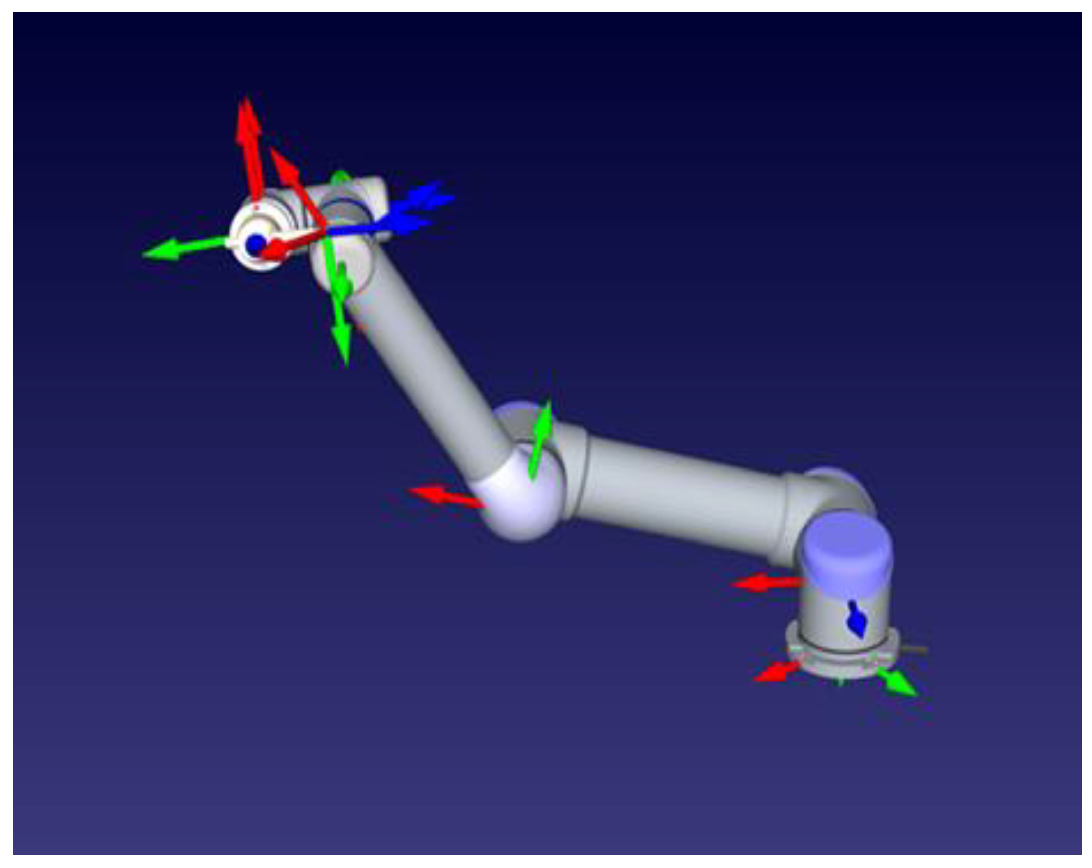
Representation of the prposed 6-DOF industrial robot and its rotation axes.
Figure 2.
Representation of the prposed 6-DOF industrial robot and its rotation axes.
Figure 3.
Robot manipulator and each joint axes sets.
Figure 3.
Robot manipulator and each joint axes sets.
Figure 4.
The proposed artificial neural network representation.
Figure 4.
The proposed artificial neural network representation.
Figure 5.
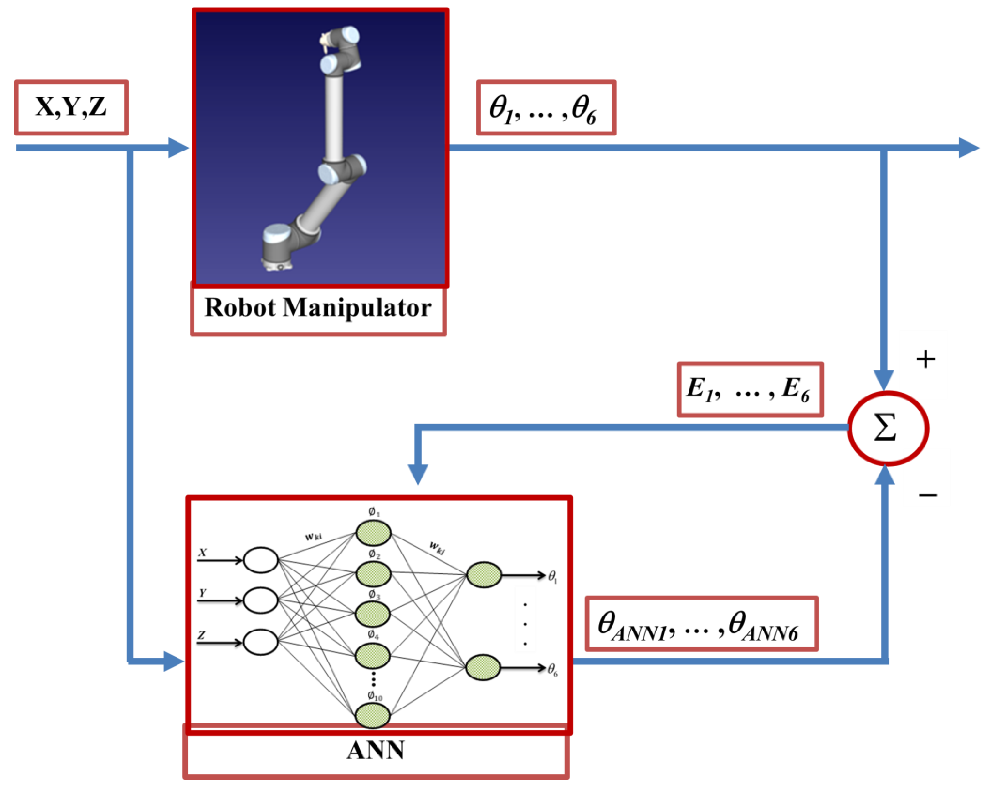
ANN based modelling of a robot manipulator.
Figure 5.
ANN based modelling of a robot manipulator.
Figure 6.
DBD learning algorithm based prediction result for the first joint angle.
Figure 6.
DBD learning algorithm based prediction result for the first joint angle.
Figure 7.
DBD learning algorithm based prediction result for the second joint angle.
Figure 7.
DBD learning algorithm based prediction result for the second joint angle.
Figure 8.
DBD learning algorithm based prediction result for the third joint angle.
Figure 8.
DBD learning algorithm based prediction result for the third joint angle.
Figure 9.
DBD learning algorithm based prediction result for the fourth joint angle.
Figure 9.
DBD learning algorithm based prediction result for the fourth joint angle.
Figure 10.
DBD learning algorithm based prediction result for the fifth joint angle.
Figure 10.
DBD learning algorithm based prediction result for the fifth joint angle.
Figure 11.
DBD learning algorithm based prediction result for the sixth joint angle.
Figure 11.
DBD learning algorithm based prediction result for the sixth joint angle.
Figure 12.
OBP learning algorithm based prediction result for the first joint angle.
Figure 12.
OBP learning algorithm based prediction result for the first joint angle.
Figure 13.
OBP learning algorithm based prediction result for the second joint angle.
Figure 13.
OBP learning algorithm based prediction result for the second joint angle.
Figure 14.
OBP learning algorithm based prediction result for the third joint angle.
Figure 14.
OBP learning algorithm based prediction result for the third joint angle.
Figure 15.
OBP learning algorithm based prediction result for the fourth joint angle.
Figure 15.
OBP learning algorithm based prediction result for the fourth joint angle.
Figure 16.
OBP learning algorithm based prediction result for the fifth joint angle.
Figure 16.
OBP learning algorithm based prediction result for the fifth joint angle.
Figure 17.
OBP learning algorithm based prediction result for the sixth joint angle.
Figure 17.
OBP learning algorithm based prediction result for the sixth joint angle.
Figure 18.
QBP learning algorithm based prediction result for the first joint angle.
Figure 18.
QBP learning algorithm based prediction result for the first joint angle.
Figure 19.
QBP learning algorithm based prediction result for the second joint angle.
Figure 19.
QBP learning algorithm based prediction result for the second joint angle.
Figure 20.
QBP learning algorithm based prediction result for the third joint angle.
Figure 20.
QBP learning algorithm based prediction result for the third joint angle.
Figure 21.
QBP learning algorithm based prediction result for the fourth joint angle.
Figure 21.
QBP learning algorithm based prediction result for the fourth joint angle.
Figure 22.
QBP learning algorithm based prediction result for the fifth joint angle.
Figure 22.
QBP learning algorithm based prediction result for the fifth joint angle.
Figure 23.
QBP learning algorithm based prediction result for the sixth joint angle.
Figure 23.
QBP learning algorithm based prediction result for the sixth joint angle.
Figure 24.
RBP learning algorithm based prediction result for the first joint angle.
Figure 24.
RBP learning algorithm based prediction result for the first joint angle.
Figure 25.
RBP learning algorithm based prediction result for the second joint angle.
Figure 25.
RBP learning algorithm based prediction result for the second joint angle.
Figure 26.
RBP learning algorithm based prediction result for the third joint angle.
Figure 26.
RBP learning algorithm based prediction result for the third joint angle.
Figure 27.
RBP learning algorithm based prediction result for the fourth joint angle.
Figure 27.
RBP learning algorithm based prediction result for the fourth joint angle.
Figure 28.
RBP learning algorithm based prediction result for the fifth joint angle.
Figure 28.
RBP learning algorithm based prediction result for the fifth joint angle.
Figure 29.
RBP learning algorithm based prediction result for the sixth joint angle.
Figure 29.
RBP learning algorithm based prediction result for the sixth joint angle.
Table 2.
D-H parameters of the Universal Robots UR5e model 6-DOF robot manipulator.
Table 2.
D-H parameters of the Universal Robots UR5e model 6-DOF robot manipulator.
| Number of Joint |
2 Link Twist Axes Angle |
Link Lenght |
Link Offset |
Joint Angle |
Joint Variable |
| i |
αi-1 |
ai-1 |
di |
Θi |
dior Θi
|
| 1 |
0 |
L1
|
0 |
Θ1
|
Θ1
|
| 2 |
0 |
L2
|
0 |
Θ2
|
Θ2
|
| 3 |
0 |
L3
|
0 |
Θ3
|
Θ3
|
| 4 |
0 |
L4
|
0 |
Θ4
|
Θ4
|
| 5 |
0 |
L5
|
0 |
Θ5
|
Θ5
|
| 6 |
0 |
L6
|
0 |
Θ6
|
Θ6
|
Table 3.
Performance comparison of the ANN network structures used.
Table 3.
Performance comparison of the ANN network structures used.
| Learning Algorithm |
ANN Network Structure |
Mean RMSE
(Training) |
Maximum RMSE
(Training) |
Mean RMSE
(Test) |
Maximum RMSE
(Test) |
| DBD |
3-10-6 |
0.427328 |
1.20820 |
0.418576 |
1.20820 |
| OBP |
3-10-6 |
0.485862 |
1.20600 |
0.507729 |
1.20600 |
| QBP |
3-10-6 |
0.373176 |
1.19047 |
0.374058 |
1.19047 |
| RBP |
3-10-6 |
1.210040 |
2.86877 |
1.267080 |
1.27537 |
| DBD |
3-5-6 |
0.726305 |
1.60402 |
0.734876 |
1.34779 |
| OBP |
3-5-6 |
0.826176 |
1.73226 |
0.804328 |
1.73226 |
| QBP |
3-5-6 |
0.878670 |
1.98618 |
0.911634 |
1.98618 |
| RBP |
3-5-6 |
1.385830 |
2.72113 |
1.523790 |
2.72113 |
Table 4.
R2 values obtained for each learning algorithm.
Table 4.
R2 values obtained for each learning algorithm.
| Learning Algorithm |
ANN Network Structure |
|
| |
|
|
|
|
|
|
|
| DBD |
3-10-6 |
0.99997 |
0.99938 |
0.99773 |
0.99932 |
0.99996 |
0.99996 |
| OBP |
3-10-6 |
0.99996 |
0.99870 |
0.99310 |
0.99953 |
0.99995 |
0.99990 |
| QBP |
3-10-6 |
0.99900 |
0.99870 |
0.99310 |
0.99953 |
0.99995 |
0.99990 |
| RBP |
3-10-6 |
0.99900 |
0.98952 |
0.98709 |
0.99426 |
0.99934 |
0.99910 |
| DBD |
3-5-6 |
0.99957 |
0.99734 |
0.99349 |
0.99853 |
0.99946 |
0.99985 |
| OBP |
3-5-6 |
0.99950 |
0.99803 |
0.99355 |
0.99824 |
0.99933 |
0.99933 |
| QBP |
3-5-6 |
0.99993 |
0.99602 |
0.99449 |
0.99595 |
0.99994 |
0.99995 |
| RBP |
3-5-6 |
0.99922 |
0.97655 |
0.96693 |
0.99360 |
0.99915 |
0.99854 |
