The design flood estimation should consider the regulation of upstream cascade reservoirs which has significantly altered downstream hydrologic regime. The current flood regional composition (FRC) methods do not consider the unfavorable reservoir operation conditions for flood prevention. In this paper, a novel framework, the most unfavorable flood regional composition (MUFRC) method, was proposed based on the flood risk analysis to estimate design flood in cascade reservoir operation period. The results of case study in Yalong River basin indicated that: (1) The proposed MUFRC method would allocate more flood volume into downstream uncontrolled sub-basin, and the precise definition of flood loss could make great difference on MUFRC method for rational estimation of design flood. (2) The 1000-year design flood peak, 3-day and 7-day flood volume of the outlet section estimated by MUFRC method are 15400 m3/s, 3.91, and 8.42 billion m3 respectively, which are all greater than values estimated by other FRC methods; (3) The reduction of design floods in reservoir operation period result the adjustment of flood control water level in downstream reservoirs, which could additionally generate 460 million kW·h (+1.82%) hydropower during flood season. Comparison study and sensitivity analysis further proves that the MUFRC method could rationally allocate flood volume and meanwhile balance the flood prevention risk and comprehensive utilization benefits, which is worth for further study and practical application.

Keywords:

Subject: Engineering - Civil Engineering

1. Introduction

The operation of cascade reservoirs has altered the downstream hydrologic regime, and the flow discharge hydrograph of flood has also significantly changed both temporally and spatially (Duan et al., 2016; Vlopi et al., 2016). Traditionally, design flood is estimated under natural flood condition in the reservoir planning and construction periods (MWR, 2006), which fails to adapt to the hydrological alteration (Guo et al., 2018). Hence how to investigate the “design flood in cascade reservoir operation period” becomes the hot research topic for effective utilization of flood water resources. Meanwhile, reservoir operation should always consider and balance the flood hazard risk and comprehensive benefits (Qi, 2017; Qi and Liu, 2018), which is well worth blending in the estimation of unfavorable downstream design flood under the regulation of upstream reservoirs (Liu et al., 2015; Zhang et al., 2019;).

There are two approaches widely applied to investigate the design flood considering the impact of climate change and human activities (primarily reservoir regulation), namely non-stationary flood frequency analysis (NFFA) method, and flood regional composition (FRC) method (Xiong et al., 2019; Xiong et al., 2020; Xie et al., 2021; Jiang et al., 2021;). The former requires measured flood data series, while the latter needs reconstructed natural flood data series. The NFFA method defines time-varying covariates relevant to influence factors of design flood and fits a time-varying distribution model (Rigby and Stasinopoulos, 2005). With the recent values of covariates input into the fitted model, the characteristic feature of design flood in operation period could be derived (López et al., 2013). The selection of covariates would significantly influence the effect and rationality of NFFA method. For example, Reservoir Index (RI), defined with reservoir capacity and catchment area, has been widely applied and successfully recognized the downward trend of downstream flood (Wang et al., 2017). But RI indicator was unable to explain why and how the design flood is reduced and which hydrological mechanism the RI-caused reduction in frequency analysis corresponded to, let alone derivation of an hourly design flood hydrograph within flood control operation and channel flow routing (Su and Chen, 2019; Xiong et al., 2020). Thus, NFFA method might be more suitable for large and complex basins with massive reservoirs, where natural flood data series are very difficult to be reconstructed.

The FRC method based on the mechanism of runoff generation and flow concentration process that allocates downstream design flood to each sub-basin (Guo et al., 2018). With the allocated floods controlled and regulated by hydraulic structures, design flood in operation period could be estimated with reservoir outflow discharge, river channel flood routing and inter-basin inflow discharge (MWR, 2006). In this way, the complicate operation rules and flood routing pattern could be constrained, and the design flood in operation period influenced by cascade reservoirs would be derived to the design section level by level. The FRC method has been widely applied in design flood estimation in China (MWR, 2006), in which the key point is how to rationally allocate downstream flood volume.

Ministry of Water Resources (MWR) of China has recommended some methods for downstream design flood estimation, among which the equivalent frequency flood regional composition (EFFRC) method was the most classic and practical one (MWR, 2006). The EFFRC method assumed that the flood frequency of upstream reservoir or inter-basins was identical with that of downstream design section. In other words, it implicitly suggested that the flood series in designative sub-basin and design-section were fully related with correction coefficient equal to one, so their cumulative distribution function (CDF) all responded to design frequency p. This basic assumption obviously neglected the uneven rainfall distribution and randomness in flood magnitudes which limited the EFFRC method to the highly correlated basins (Xiong et al., 2020). Besides, the number of EFFRC schemes exponentially increased with the number of reservoirs, which also made the selection of representative EFFRC scheme more difficult. Guo et al. (2018) proposed the most likely flood regional composition method (MLFRC) with the maximum probability of flood allocation to investigate downstream design flood, which was proved to be more reasonable and practical through statistical experiments. The copula functions were also introduced into MLFRC method to describe the joint distribution of flood volumes from various sub-basins. The application of EFFRC and MLFRC methods suggested that the upstream reservoir regulation has significantly reduced the flood peak and volume in the downstream section, and thus the flood control water level in reservoir operation period might need a reevaluation owing to the differences between design flood hydrographs in reservoir construction and operation period (Guo et al., 2018; Xiong et al., 2019).

The current FRC methods tended to derive a rational flood volume allocation scheme in view of probability and statistic analysis, and neglected to consider flood prevention risk under unfavorable situation. Hence, this paper proposed a novel FRC method, i.e., the most unfavorable flood regional composition (MUFRC) method, which consider the flood occurrence probability and flood disaster loss. The flood occurrence probability could be effectively estimated by copula functions which has been confirmed in various hydrological analysis fields (Lee et al., 2018; Yin et al.; 2018), while the flood disaster loss still required a reasonable definition. Since flood damage is tightly associated with flood discharge and duration (Zhao et al., 2024; Zhang et al., 2023;), the additional suffered flood volume was selected and used to symbolize the flood loss in this study, which was exactly the integral and comprehensive reflection of the two damage factors.

The additional suffered flood volume was furtherly categorized as excessive flood volume from the uncontrol inter-basins. Flow discharge from the sub-basin next to design section would not be regulated by any reservoirs, which was nonnegligible but always ungagged. MWR (2006) has suggested that flood volumes from these uncontrol basins were worth particular attention in FRC method. Hence, this paper defined the uncontrolled flood loss with the part of flood volume above designed controllable value. With quantified flood loss, MUFRC method would solve the maximum product of it and probability density, derive and then allocate the FRC scheme into each sub-basin for design flood estimation.

The aim of this study was to propose a novel framework for the investigation of the most unfavorable design flood in cascade reservoir operation period. The rest of the paper was organized as follows: Section 2 briefly introduced the proposed MUFRC and other methods. In Section 3 the cascade reservoirs in Yalong River basin were selected as the case study to demonstrate the effectiveness of the proposed methods, and the most unfavorable design flood and corresponding reservoir flood control water levels were derived, whose hydropower generation benefits were reevaluated correspondingly. Section 4 further discussed and compared different methods under different flood scenarios. Finally, the conclusions were given in Section 5.

2. Methodology

2.1. Copula Function

Assuming that there were random variables X₁, X₂, …, X_n, whose marginal distribution functions could be respectively expressed as F₁(X₁), F₂(X₂), …, F_n(X_n), and the joint distribution function was expressed as H(x₁, x₂,…, x_n). Then according to Sklar’s theorem, there was a function C satisfying the following equation (Nelson, 2006):

H (x_{1}, x_{2}, ..., x_{n}) = C (F_{1} (x_{1}), F_{2} (x_{2}),, ..., F_{n} (x_{n}))

(1)

The function C was called Copula function. Represent F₁(X₁), F₂(X₂), …, F_n(X_n) with u₁, u₂, …, u_n, and let x_i=F_i^-1(u_i), the Eq. (1) could be rewritten as (Salvadori and De Michele, 2004; Salvadori et al., 2016):

C (u_{1}, u_{2}, ..., u_{n}) = H (F_{1}^{- 1} (u_{1}), F_{2}^{- 1} (u_{2}), ..., F_{n}^{- 1} (u_{n})) = H (x_{1}, x_{2}, ..., x_{n})

(2)

Hence, the joint probability density function of H could be derived as:

f (x_{1}, x_{2}, ..., x_{n}) = \frac{\partial^{n} C (u_{1}, u_{2}, ..., u_{n})}{\partial x_{1} \partial x_{2}, ..., \partial x_{n}} = c (u_{1}, u_{2}, ..., u_{n}) \prod_{i = 1}^{n} f_{x_{i}} (x_{i})

(3)

where c denoted the mixed partial derivative of C. In flood frequency analysis, Archimedean copulas were always applied to bivariate simulation, while t-copula and vine copula were more recommended for high dimension systems (Xiong et al., 2019).

2.2. Flood Regional Composition (FRC) Method

Cascade reservoirs have significantly altered downstream hydrologic regime, and made a great difference on the design flood hydrograph. FRC method could reallocate the original design flood in construction period into each sub-basin according to representative flood volume rates. And with the simulation of flood control and routing from upstream to downstream, design flood hydrograph in operation period could finally be derived.

Sketch diagram of FRC method was shown in Figure 1. A cascade reservoir system composed of n reservoirs divided the basin into n+1 sub-basin. As shown in Figure 1, A_i, B_i and C represented the i-th upstream reservoir, the i-th inter-basin, and the design section respectively, whose inflows were respectively represented as random variables X_i, Y_i and Z with corresponding values x_i, y_i and z.

2.3. Equivalent Frequency Flood Regional Composition (EFFRC) Method

Generally, the equivalent frequency floods are more likely to occur among highly correlated adjacent sub-basins. EFFRC method recommended by the MWR (2006) has been widely used and proved to be a convenient reference in practice. Take single reservoir system as an example for illustration:

(1) If both the design floods in downstream section and upstream reservoir were equal in design frequency p, and their flood volumes were represented as z_p and x_p. Then according to the principle of water balance corresponding flood volume y at inter-basin B is given by z_p-x_p. So [x_p, z_p-x_p] was one of EFFRC schemes for single reservoir system.

(2) If design floods in downstream section and interval basin B were equal in frequency, then similarly, flood volume X at upstream reservoir A site was given by x=z_p-y_p. And [z_p–y_p, y_p] was the other EFFRC scheme for single reservoir system.

[x_p, z_p-x_p] and [z_p–y_p, y_p] served as the basic schemes for EFFRC method. And for the cascade reservoir system, as the number of reservoirs (n) increased, the research basin could be divided into n single reservoir sub-systems from downstream to upstream one by one, then the number of EFFRC schemes (2ⁿ) would increase dramatically based on the possible choice of basic schemes in each sub-system.

2.4. Most Likely Flood Regional Composition (MLFRC) Method

Probability density of the FRC scheme (x₁, y₁, y₂,…, y_n) was estimated by copula ,whose higher value was considered more reasonable and representative in MLFRC method. Hence, the MLFRC scheme could be obtained when copula-fitted joint distribution f(x₁, y₁, y₂,…, y_n) was maximized within the principle of water balance (Guo et al., 2018):

\begin{array}{l} \begin{matrix} m a x \end{matrix} f (x_{1}, y_{1}, \dots, y_{n - 1}, y_{n}) = c (u_{1}, v_{1}, ..., v_{n - 1}, v_{n}) f_{X_{1}} (x_{1}) \prod_{i = 1}^{n} f_{Y_{i}} (y_{i}) \\ s t . \begin{matrix} x_{1} + \sum_{i = 1}^{n} y_{i} = z_{p} \end{matrix} \end{array}

(4)

where u₁ and v_i denoted the corresponding CDFs of x₁ and y_i; f_X₁(x₁) and f_Yi(y_i) denoted the marginal distributions of floods at upstream reservoir A₁ and each inter-basin B_i, respectively; c(·) denoted the derivative of copula function. Xiong et al. (2019) recommended the genetic algorithm (GA) to solve the MLFRC method for high-dimension cascade reservoir system with the flood volumes in each sub-basin coded and optimized, in which the principle of water balance served as the constraint condition to prevent unrealistic solutions.

2.5. Most Unfavorable Flood Regional Composition (MUFRC) Method

The EFFRC method searched the composition of flood volumes whose CDFs were equal to design frequency, implicitly assuming that the flood data series in all sub-basins were completely linearly correlated. The MLFRC method tended to search the scheme with the highest probability density, which was able to fully consider the correlation of flood generation (Xiong et al., 2020). This section proposed MUFRC method based on flood prevention risk analysis.

There were various mathematical definitions of risk R. The United Nations Department of Humanitarian Affairs (1992), now reorganized as the United Nations Office for the Coordination of Humanitarian Affairs, stated that risk was the product of hazard and vulnerability. Sun et al. (2017) and Qi (2017) pointed out that for flood prevention risk, the hazard was usually described by the probability of occurrence P_R, and the vulnerability was embodied as the disaster loss D_R. Hence, the risk for a specific flood disaster event could be quantified as R=P_R×D_R.

The probability of occurrence P_R could be effectively estimated by Eq.(4), similar to above MLFRC method, while the disaster loss D_R was very difficult to be accurately estimated. Generally, the flood disaster loss was tightly associated with the additional suffered flood at the downstream flood control section. Since the essence of the FRC method was the rational allocation of flood volumes, the flood vulnerability was set as the excessive flood volume from uncontrolled sub-basins in this paper. As shown in Figure 1, the flood volumes X₁, Y₁, …, Y_n_-1 from upstream basins would be regulated by cascade reservoirs, while Y_n directly threatened flood security of downstream section (MWR, 2006). Hence the more the flood volume allocated in the uncontrolled sub-basins, the larger uncontrolled flood loss was. Therefore, disaster loss D_R was defined as follows:

\begin{array}{l} D_{R} = Δ y_{n} \\ Δ y_{n} = \{\begin{matrix} \begin{matrix} y_{n} - y_{n}^{E} & y_{n} - y_{n}^{E} > 0 \end{matrix} \\ \begin{matrix} 0 & y_{n} - y_{n}^{E} \leq 0 \end{matrix} \end{matrix} \end{array}

(5)

where

y_{n}^{E}

denoted the flood volume assigned to the n-th uncontrolled sub-basins in the EFFRC method, which was exactly regarded as the designed controllable flood volume for downstream section; Δy_n denoted additional suffered uncontrolled flood volume. Then, the MUFRC scheme (

x_{1}^{U}

y_{1}^{U}

y_{2}^{U}

, …,

y_{n}^{U}

) could be solved by the following equation:

\begin{array}{l} \max \begin{matrix}  \end{matrix} R = Δ y_{n} \cdot f (x_{1}, y_{1}, ..., y_{n}) \\ s t . \begin{matrix} x_{1} + \sum_{i = 1}^{n} y_{i} = z_{p} \end{matrix} \end{array}

(6)

2.6. Design Flood Estimation in Cascade Reservoir Operation Period

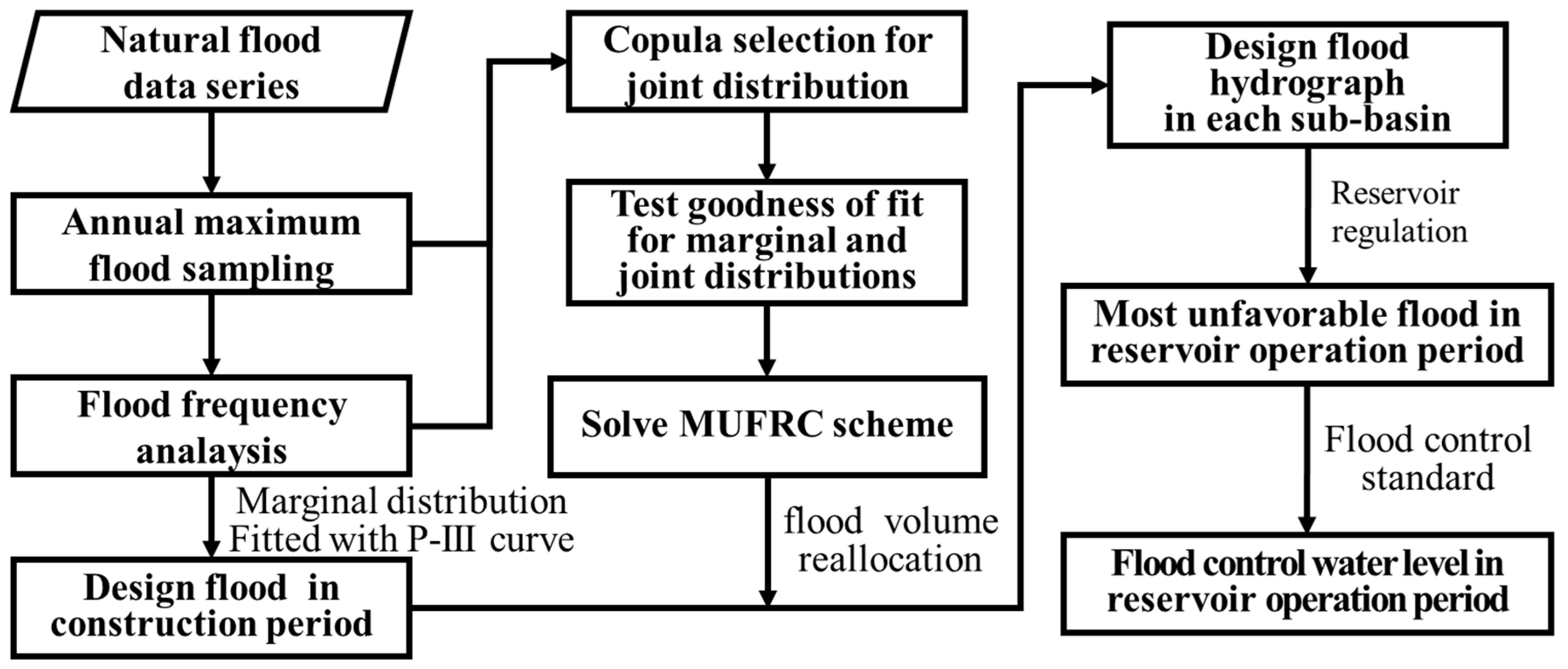
Figure 2 represented the estimation procedure of the most unfavorable design flood in reservoir operation period. Firstly, similar to traditional frequency analysis, the marginal distributions should be fitted with P-III curves based on natural annual maximum flood (MWR, 2006); Then fit the joint distributions with copula, and solve the MUFRC method; Allocate design flood with the MUFRC scheme for each sub-basin and input into reservoir operation system; Finally, design flood in reservoir operation period was estimated and the flood control water level could be derived.

3. Case Study

3.1. Cascade Reservoirs in the Yalong River Basin

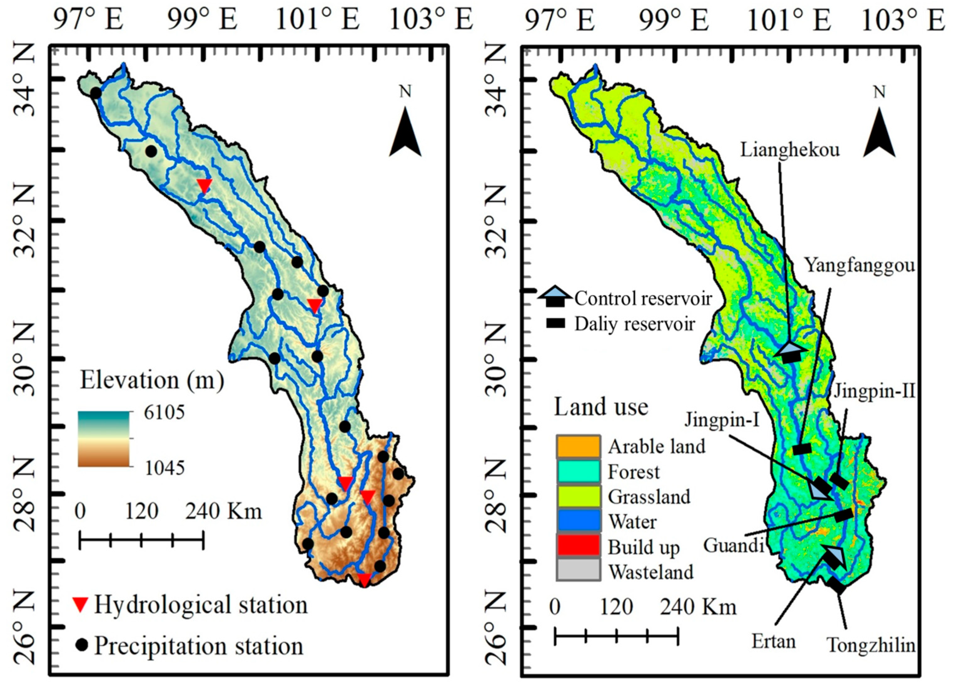
The Yalong River is located in the east of the Qinghai-Tibet Plateau, China, with a geographical location between 26° 32’ and 33° 58’ N, 96° 52’ and 102° 48’ E. As the largest tributary of upper Yangtze River, its entire basin is shaped like a north-south strip, with an average width of about 137 km. The elevation varies from 5400 m to 980 m above sea level, which gathers 33.72 million kW theoretical hydropower resources for development and utilization. And the Yalong River Hydropower base ranks the third in the “China’s Thirteen Largest Hydropower Base Plan”. Figure 3 showed the location of seven reservoirs that have been built in the middle and low reaches of the Yalong River along the mainstream, and Table 1 listed the basic information of them, namely, Lianghekou (LHK), Yangfanggou (YFG), Jinping-1 (JP1), Jinping-2 (JP2), Guandi (GD), Ertan (ET), and Tongzilin (TZL) (He et al., 2023). All of seven reservoirs are constructed for the purpose of hydropower generation, among which LHK, JP1 and ET are the main controlled reservoirs additionally designed for flood control. A total of 4.5 billion m³ flood control storage capacity has allocated as 2.0, 1.6, and 0.9 billion m³ for LHK, JP1, ET, respectively.

In this section, flood volume of Yalong River basin could be distributed into the LHK reservoir, L-J inter-basin, J-E inter-basin, and E-T inter-basin according to three controlled reservoir and downstream outlet section TZL. The 1000-year design flood was estimated and compared with original value, since these dams were designed and built for preventing 1000-year design floods in reservoir construction period.

3.2. The Marginal Distribution of Flood Data Series

According to the characteristics of runoff and cascade reservoirs in the Yalong River basin, 7d flood hydrograph deduced with 7d flood volume in TZL section was important for the flood control. P-III curve was chosen to depict the marginal distribution of 7d flood volume series, which was commonly used in China for design floods in construction period (MWR, 2006). The density function of P-III distribution is expressed as follows:

f (x) = \frac{β^{α}}{Γ (α)} {(x - a_{0})}^{α - 1} e^{- β (x - a_{0})}

(7)

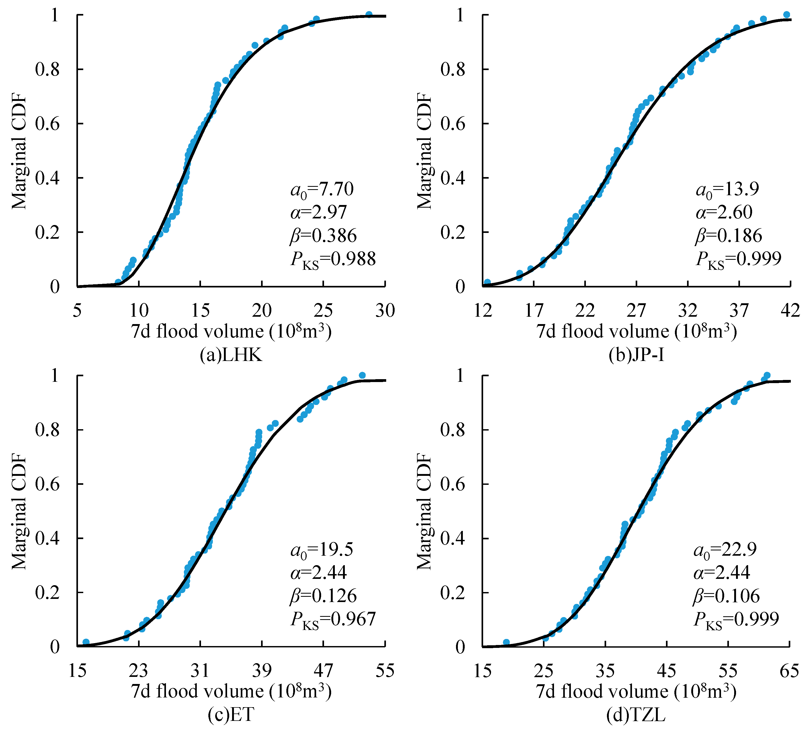
where a₀, α and β are the location, shape and scale parameters of the P-III distribution, respectively. For illustration only, the marginal CDF of 7d flood volumes for LHK, JP1, ET, TZL were plotted in Figure 4, respectively.

The sample points (blue point) fell within a narrow range of theoretical distribution curve (black line), and all passed the Kolmogorov–Smirnov test within the 5% significance level (P_KS>0.05), both of which confirmed that P-III distribution could fit the marginal distribution of flood series well.

3.3. The Joint Distribution of Flood Data Series

Archimedean copula, t-copula and vine copula were sequentially applied to fit the joint distributions of design flood at TZL section. The functions of Gumbel copula (C_G), Clayton copula (C_C), Frank copula (C_F), and t-copula (C_T) are expressed by following equations, respectively:

\begin{matrix} C_{G} (u, v) = \exp \{- {[{(- \ln u)}^{θ} + {(- \ln v)}^{θ}]}^{1 / θ}\} & τ = 1 - 1 / \end{matrix} θ

(8)

\begin{matrix} C_{C} (u, v) = （ u^{- θ} + v^{- θ} - 1 ）^{1 / θ} & τ = θ / (θ + 2) \end{matrix}

(9)

\begin{matrix} C_{F} (u, v) = - \frac{1}{θ} \ln [1 + \frac{(e^{- θ u} - 1) (e^{- θ v} - 1)}{e^{- θ} - 1}] & τ = 1 + \frac{4}{θ} \end{matrix} [\frac{1}{θ} \int_{0}^{θ} \frac{t}{\exp (t) - 1} d t - 1]

(10)

C_{T} (u_{1}, u_{2}, ..., u_{n}; Σ, v) = T_{Σ, v}^{- 1} (T_{v}^{- 1} (u_{1}), T_{v}^{- 1} (u_{2}), ..., T_{v}^{- 1} (u_{n}))

(11)

where τ denoted Kendall’s tau coefficient, θ denoted the parameter of copula function; T_v^-1 and T_Σ,v^-1 denoted the inverse functions of t-distribution for univariate and multivariable, respectively; v denoted the degree of freedom; Σ denoted correlation matrix. Vine copula could be expressed with the topological connections among other basic copulas.

The primary criterion for evaluating the goodness of fit was the least value of Akaike Information Criterion (AIC), which was defined as follows:

AIC = 2 k + 2 \ln RMSE

(12)

where k denoted the count of copula parameters; RMSE denoted the rout mean square error between empirical and theoretical frequencies.

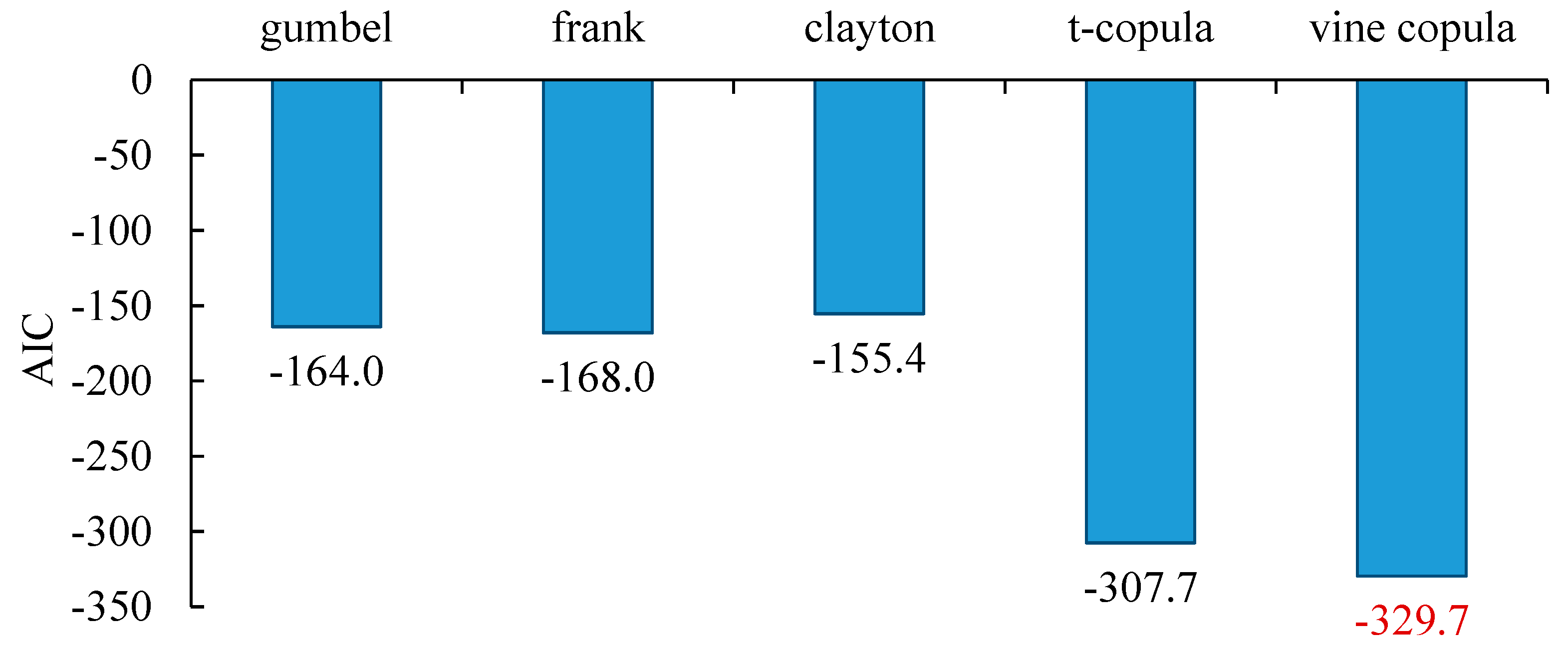
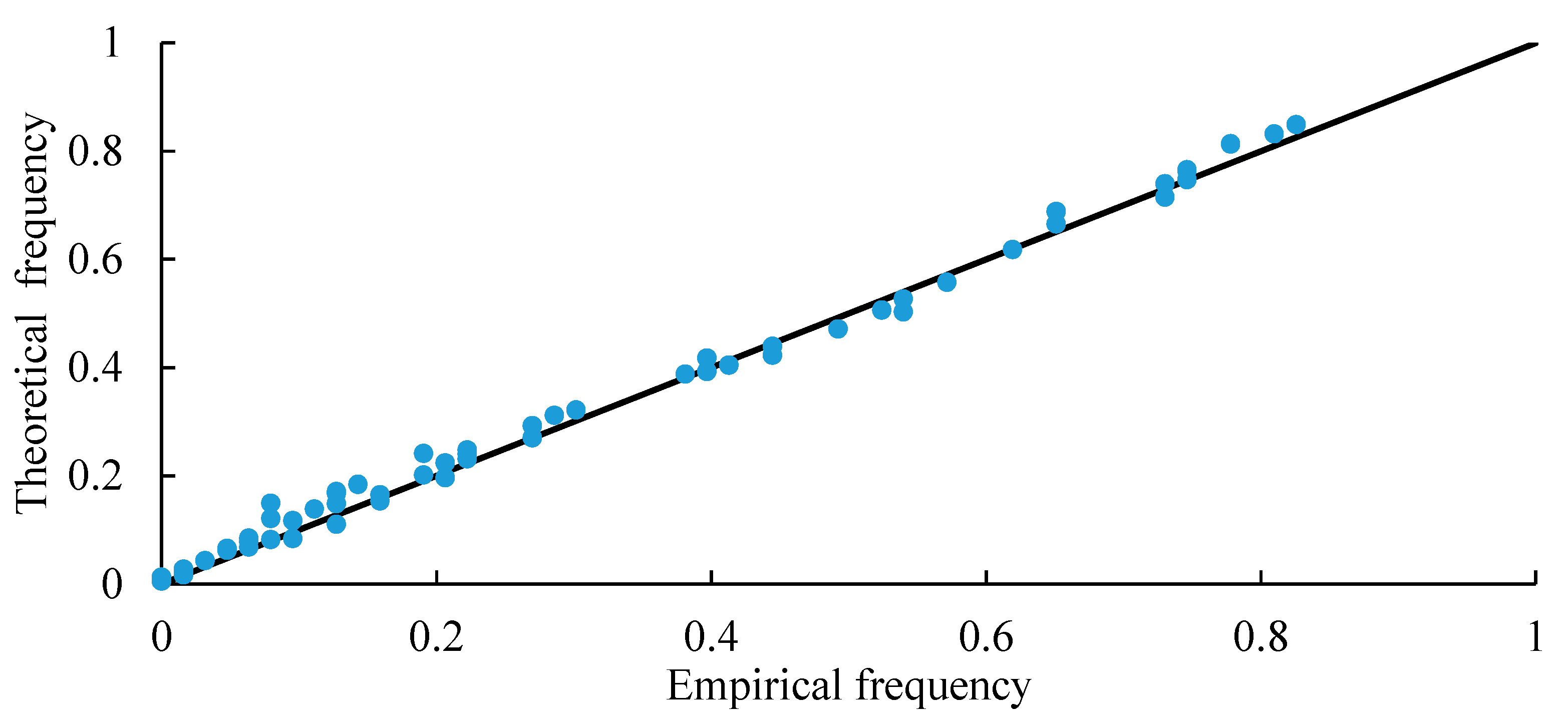
As shown in Figure 5 vine copula described the joint distribution of 7d flood volume from each sub-basin most accurately with minimum AIC. The P-P plot of the theoretical and empirical CDFs shown in Figure 6 also indicated that the series conformed to the specified vine copula with the scatters narrowed around the 1:1 line.

3.4. Design Flood Estimated by Various FRC Methods

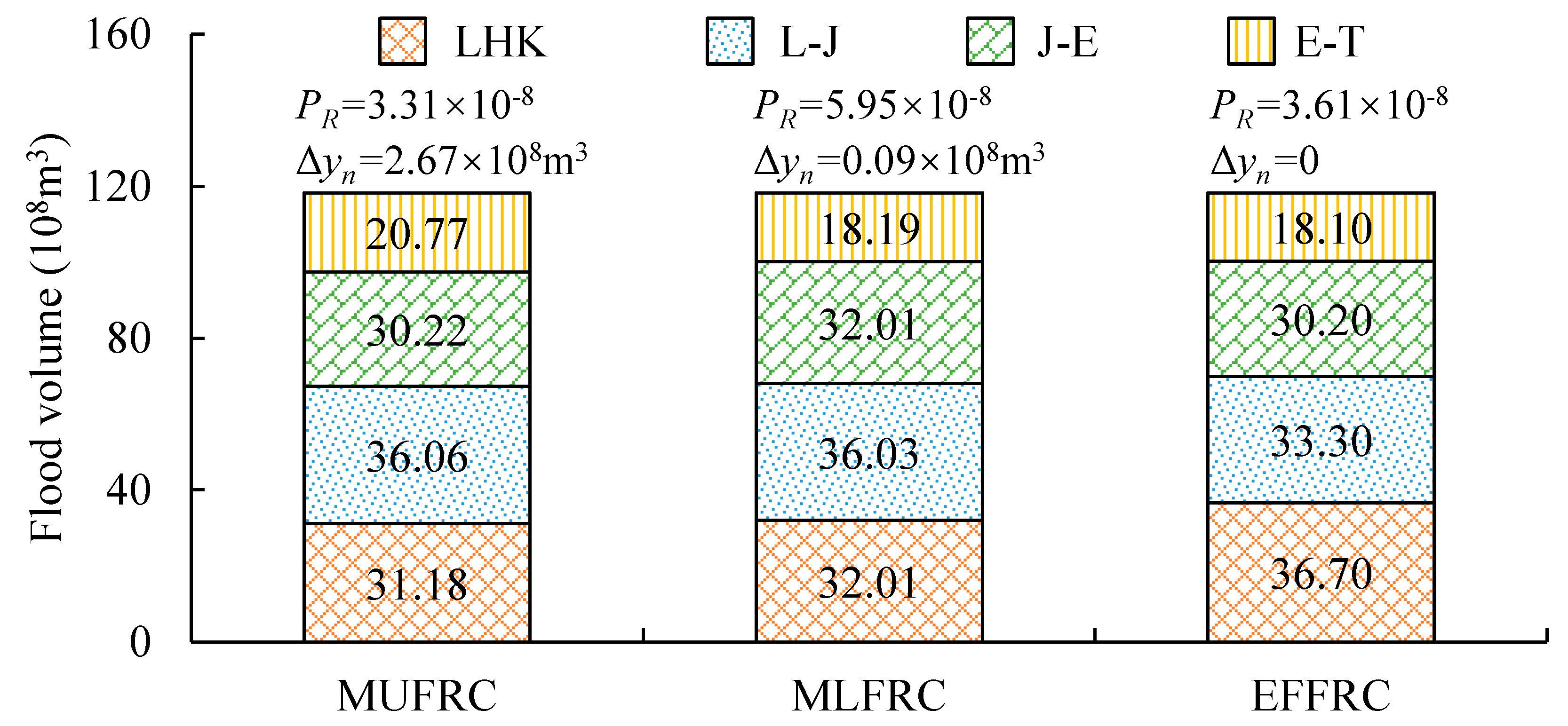
After selected the marginal and joint distributions, the GA algorithm was applied to solve the FRC methods, whose parameters were set as follows: population size = 100, generation = 500, crossover rate = 0.95 and mutation rate = 0.05. The EFFRC, MLFRC and MUFRC schemes at TZL section were listed and compared in Figure 7. It is worth mentioning that Yalong River is located in mountain region with high correlation between floods in adjacent sub-basins, whose Pearson correlation were between 0.72 and 0.97. Therefore, significant difference should not be observed among those FRC schemes. (Details about FRC difference and Pearson correlation will be discussed in Section 4.3.)

The EFFRC method implicitly assumed the Pearson correlation coefficient of flood series equals to one for corresponding sub-basins, which was obviously not rational in real case. For Yalong River basin, the EFFRC schemes tended to allocate more flood into upstream reservoir and less for downstream inter-basin. Meanwhile, MLFRC fully considered the correlation and occurrence pattern of floods in each sub-basin, and allocated more flood into J-E and E-T sub-basin. As defined in Eq. (6), the MUFRC modified MLFRC method with the weight of additional suffered flood at downstream section. Hence, the MUFRC scheme allocated more flood volume into E-T inter-basin which is unfavorable for flood prevention.

By allocating the original design flood in construction period with the flood volume rates of various FRC schemes to each sub-basin and inputting them into the cascade reservoir operation system in Yalong River basin, the design flood in reservoir operation period could be obtained. The design flood hydrographs were shown in Table 2 and Figure 8. The results indicated that:

(1) The full utilization of flood control storage in upstream reservoirs has significantly changed the flood characteristic features at downstream section. Compared with original designed values, the annual maximum peak discharge Q_max, W₁, W₃, and W₇ flood volumes estimated by MUFRC scheme at TZL design section would decrease by 36.6%, 36.1%, 33.0% and 28.7%, respectively.

(2) Traditionally, flood control standard defined the highest water level during the simulating operation of design flood as design flood water level, which started from flood limit water level. Since the downstream flood control pressure has been alleviated by upper cascade reservoirs, the original flood limit water level might fail to adapt to these alterations and could be redesigned for more benefits. Through flood control estimation, the water levels of downstream controlled reservoirs like JP1 and ET could be appropriately derived as 1862.39 m and 1192.59 m for MUFRC scheme within the unchanged flood control standard and security requirement, which increased by 3.39 m and 2.59 m compared with original flood limit water level.

(3) The raise of flood control water level would correspondingly increase the net head of hydropower generator units, and was also helpful for irrigation, shipping and hydro-ecology. Input the raised water levels as boundary constrains, and simulate long-term cascade reservoir operation with runoff data series during the flood season, then the power generation output of the cascade reservoir system could be assessed. The redesigned water level could increase the total of hydropower generation (HG) in Yalong River basin from 45.58 to 46.22 billion kW·h (+1.82%) during the flood season, indicating a significant raise of economic benefits.

The flood allocation of EFFRC method would make full use of upstream reservoir storage for flood control, so its design flood and flood risk were the least. The minimum flood peak indicated that EFFRC method was unsuitable for unfavorable conditions. As shown in Figure 7, the flood risk in MLFRC scheme was also insignificant with small value of Δy_n, and its probability density was not so much greater than other FRC schemes, which still failed to meet the security requirement of design flood. As its definition, MUFRC schemes would result in the greatest flood hazard risk and allocated the largest 7d flood volume into E-T sub-basin, whose R=P_R×Δy_n was almost 17 times than MLFRC results. Since MUFRC-estimated volumes for LHK, L-J and E-T sub-basins were respectively similar to those in MLFRC, MLFRC, and EFFRC as shown in Figure 7, where the design flood were similarly regulated by the upstream reservoirs. Therefore, the additional flood volume in E-T inter-basin made the difference on those FRC schemes. Meanwhile, the probability density remained acceptable which was just slightly less than EFFRC method. Hence, the MUFRC scheme was preferred for the estimation of design flood in cascade reservoir operation period.

4. Discussion and Comparison

4.1. Influence of Flood Loss

The flood loss D_R distinguished MUFRC method from MLFRC method. An unsensitive definition of D_R would make MUFRC scheme similar to MLFRC. On the contrary, violently fluctuating D_R would lead to unrealistic results. This section aimed to investigate how flood loss D_R and relevant definition indicator

y_{n}^{E}

would influence results of MUFRC method.

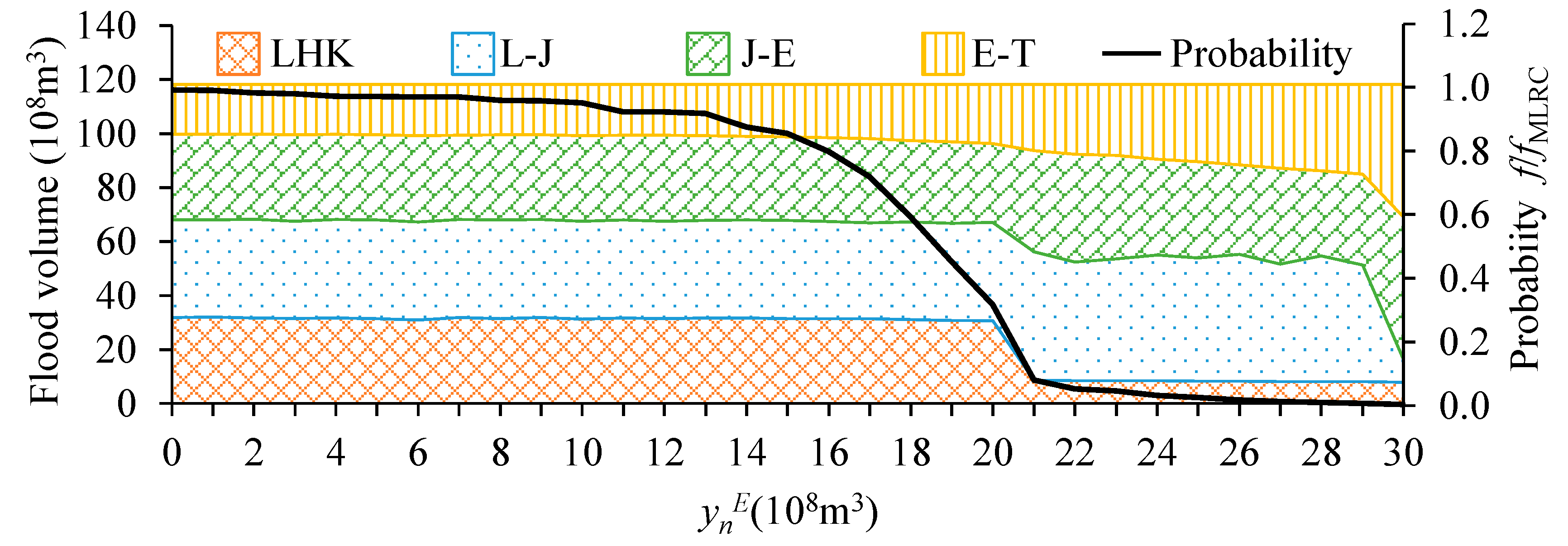
As shown in Figure 9, controllable flood volume

y_{n}^{E}

made a great difference in the MUFRC method. If

y_{n}^{E}

<1.5 billion m³, little fluctuation could be recognized for different MUFRC schemes, and their probability densities approximated to that of MLFRC, which indicated that the probability dominated the quantification of uncontrolled flood risk rather than the magnitude of uncontrolled flood. On the contrary, if

y_{n}^{E}

>2.0 billion m³, the steep decreases of allocated flood for LHK reservoir and occurrence probability suggested an unsatisfying MUFRC results, which came to worse if

y_{n}^{E}

>2.9 billion m³ that the downstream J-E and E-T sub-basins carved up more than 80% flood volume. Stringent flood security requirement might lead to high

y_{n}^{E}

, indicating that the downstream section could suffer more flood. Then flood hazard event and flood loss of downstream section would be less likely to occur (f/f_MLFRC <0.2), so the MUFRC schemes tended to extreme solutions that allocated most flood for J-E and E-T inter-basin and especially less for LHK reservoir whose flood volume would be controlled and reduced by all three cascade reservoirs. And if 1.5 billion m³<

y_{n}^{E}

<2.0 billion m³, the flood volumes were divided just slightly more for E-T and less for other upstream basins, which were more acceptable with the 0.3~0.8 f/f_MLFRC as the flood were highly correlated in Yalong River basin. Anyway, the practical

y_{n}^{E}

=1.81 billion m³ in case study, and MUFRC scheme differed from MLFRC and presented a reasonable possibility (f/f_MLFRC = 0.55), so the case study remained rational and applicative.

4.2. Sensitivity Analysis

The Bootstrap method was applied for sensitivity analysis of FRC methods: Firstly, generate the flood series based on the fitted distributions for Yalong River basin; Then, reassess the marginal and joint distributions with generated sample series and derive the corresponding FRC schemes; Finally, repeat above two steps for sufficient times and analyze the statistic features of all FRC results.

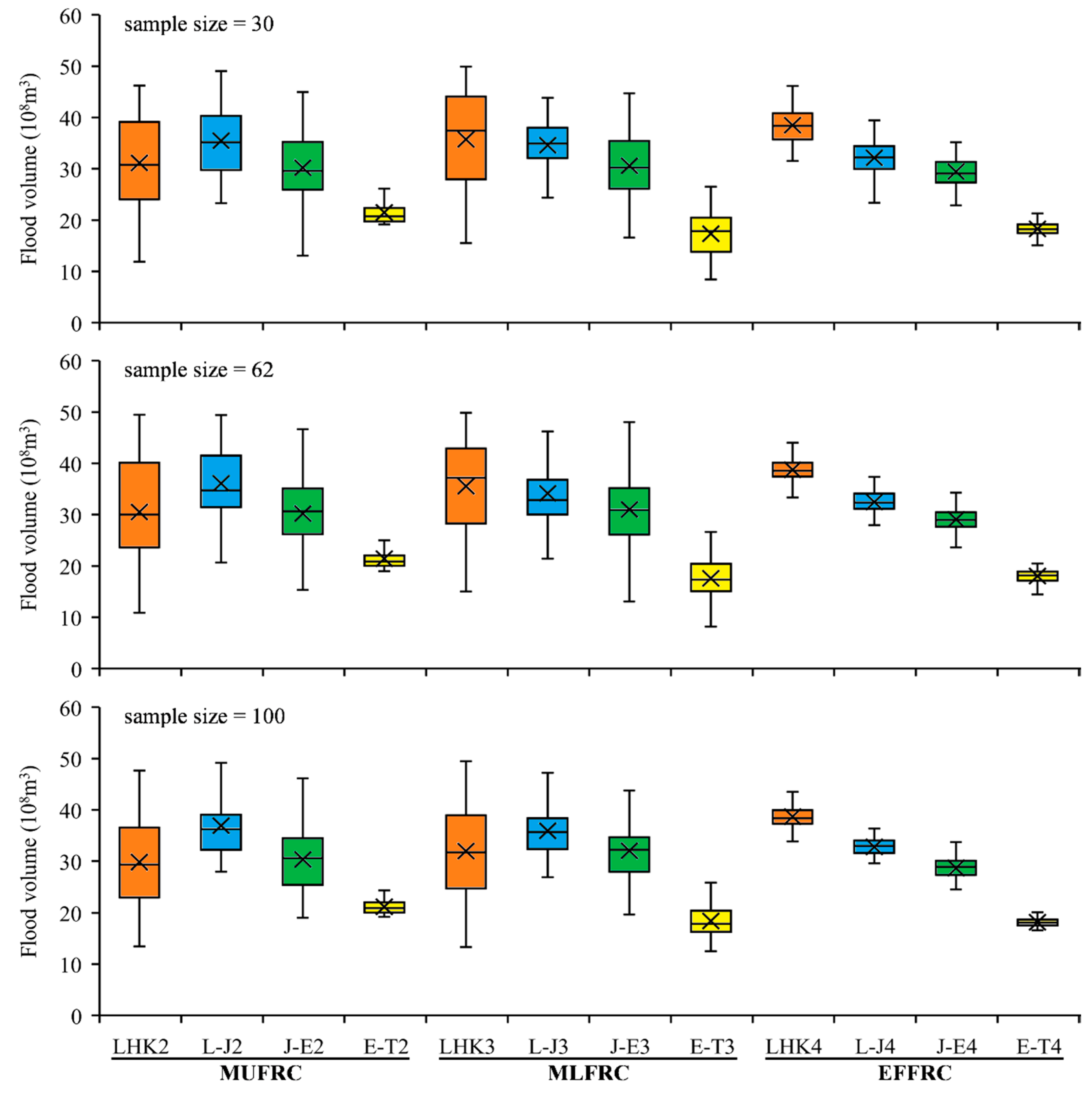
The boxplot in Figure 10 presented the flood volumes in each sub-basin for three FRC methods. Overall, the result of Bootstrap method still followed the pattern of case study. EFFRC method preferred to allocate more flood to upstream, MLFRC method tended to derive proportionate results, and MUFRC method focused more on downstream sub-basins. Meanwhile the Inter-Quartile Ranges (IQRs) were also proportional to the magnitude of floods from the inter-basins except LHK. The upper and lower edges of LHK boxes were even close to the feasible region (1~5 billion m³) set in GA algorithm, since the principle of water balance constraint x₁=z_p-y₁-y₂-y₃ mathematically led to higher statistical variance.

The sample sizes were set as 30, 62 and 100, which respectively symbolized the minimum series length requirement (MWR, 2006), the actual value in case study and an abundant sample size. Obviously, the larger the sample size, the narrower the box, especially for J-E and E-T inter-basins in Figure 10. And EFFRC method suggested less dependency on abundant sample size as its flood volume distribution were centralized with the least IQR, which was contributed to the concise mathematical definition of EFFRC method only concerned with marginal distributions except copula-fitted joint distribution and complex flood loss. The simple calculation procedure could make EFFRC method a convenient way for rough but steady design flood estimation.

The MLFRC and MUFRC method were highly sensitive to the uncertainty from copula function. In the sample size of case study shown in Figure 10 (b), IQR of E-T inter-basin was 0.20, 0.53 and 0.18 billion m³ respectively for MUFRC, MLFRC and EFFRC methods. The difference of joint distributions in Bootstrap loops directly influenced the MLFRC results, whose variable amplitude was nearly three times more than EFFRC. However, MUFRC method presented better results as its flood loss in Eq. (5) constrained flood volume in E-T inter-basin and made it strictly greater than

y_{n}^{E}

. Therefore, its lower edge and lower quartile were both close to 1.81 billion m³. In other words, the uncontrolled flood risk narrowed the feasible region of MUFRC method for GA algorithm, the uncertainty of MUFRC was relatively smaller.

The relative error RE is used to assess the accuracy of Bootstrap results, which is expressed as follow:

R E = \sqrt{\frac{{(1 - {\hat{x}}_{1} / x_{1})}^{2} + \sum_{i = 1}^{n} {(1 - {\hat{y}}_{i} / y_{i})}^{2}}{n + 1}}

(13)

where x₁ and y_i were FRC schemes derived in case study;

{\hat{x}}_{1}

and

{\hat{y}}_{i}

were FRC schemes estimated in each loop of Bootstrap. The average of RE in MUFRC, MLFRC and EFFRC methods were respectively 0.20, 0.23 and 0.07 with sample size = 62, so the instability of copula fit also led to great RE in MUFRC and MLFRC methods. And meanwhile, the risk definition helped MUFRC present better accuracy than MLFRC. 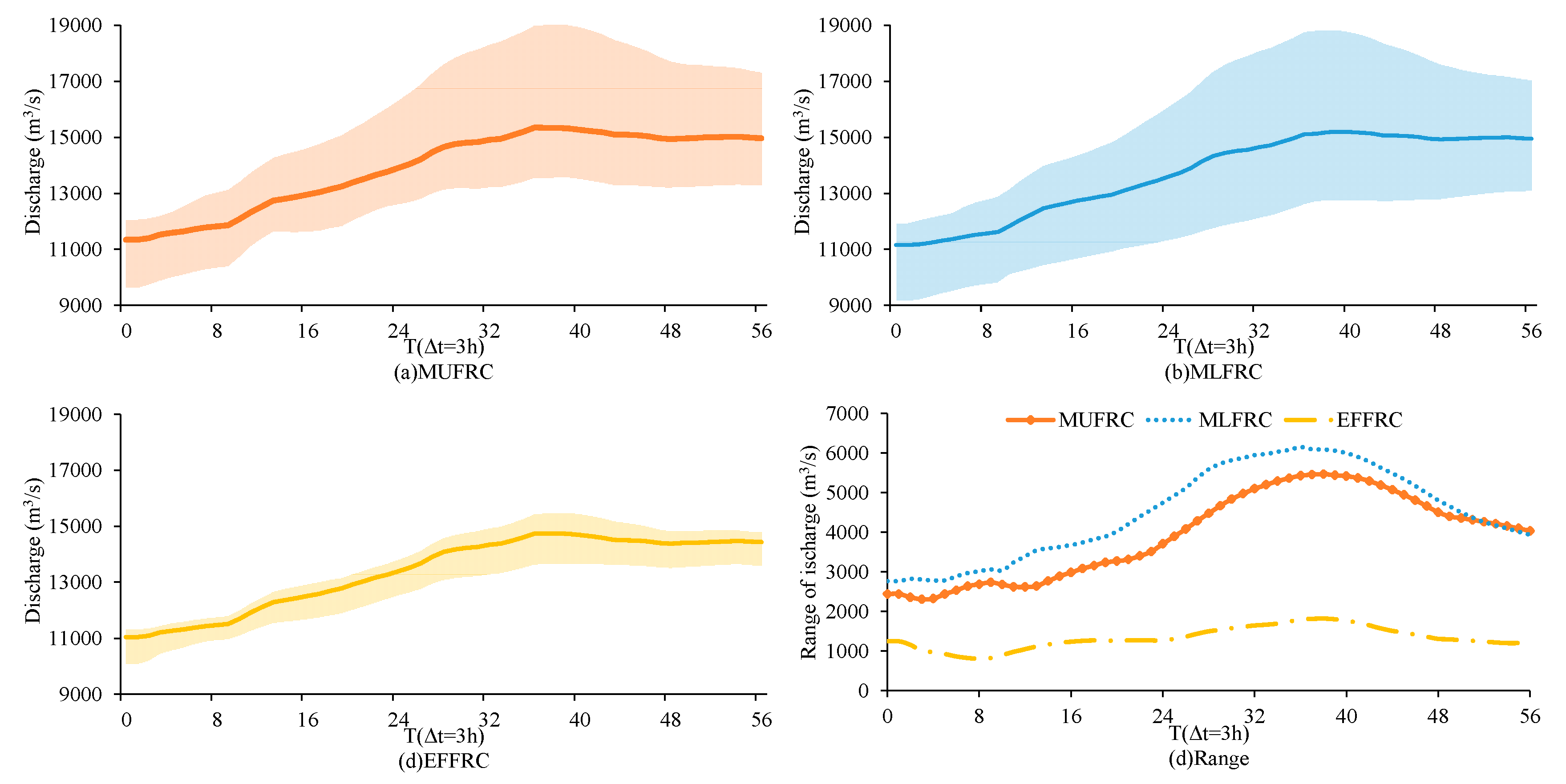Furtherly, estimate the design floods with all generated FRC schemes as shown in Figure 11. The average Euclidean distances between Bootstrap results and case study results were 6350 m³/s, 7500 m³/s, and 2070 m³/s for the three FRC methods. Besides, higher discharge corresponded to wider fluctuation range especially around flood peak. The range of MUFRC method was always narrower than that of MLFRC method, and their overlap during flood reduction period (T>50×3h) in Figure 11(d) indicated consistent reservoir flood control operation at the end of flood events.

In summary, though EFFRC method presented optimal stability, its allocation scheme made full use of upstream reservoir capacities and derived minimum design flood, which failed to fit the unfavorable security requirement. MLFRC method allocated flood with the correlation, but its probability density was the highest together with instability. MUFRC method reasonably focused on uncontrolled basin and led to the most threatening flood risk, meanwhile it overcame the incorrect assumption in EFFRC and reduced the fluctuation from copulas like MLFRC to some extent. Thus, the MUFRC was more suitable for the reference of design flood estimation.

4.3. Theoretical Derivation

In order to discuss the reasonableness of the flood risk in MUFRC, the theoretical derivation compared the analytical solutions of EFFRC, MLFRC and MUFRC methods. A two-dimensional case was taken as an example for simplification, assuming that there were floods from reservoir X and design section Z, which both obeyed normal distribution respectively, while their joint density function obeyed bivariate normal distribution (Xiong et al., 2020):

\begin{array}{l} f (x) = \frac{1}{σ_{x} \sqrt{2 π}} \exp [- \frac{{(x - u_{x})}^{2}}{2 σ_{x}^{2}}] \\ f (z) = \frac{1}{σ_{z} \sqrt{2 π}} \exp [- \frac{{(z - u_{z})}^{2}}{2 σ_{z}^{2}}] \\ f (x, z) = \frac{\exp \{- \frac{1}{2 (1 - r^{2})} [\frac{{(x - u_{x})}^{2}}{σ_{x}^{2}} - \frac{2 r (x - u_{x}) (z - u_{z})}{σ_{x} σ_{z}} + \frac{{(z - u_{z})}^{2}}{σ_{z}^{2}}]\}}{2 π σ_{x} σ_{z} \sqrt{1 - r^{2}}} \end{array}

(14)

where u_x, u_z and σ_x, σ_z denoted the average and standard deviation of X and Z, respectively; r denoted the Pearson correlation coefficient between X and Z.

Assuming that the allocation schemes for EFFRC and MLFRC were (x^E, y^E) and (x^L, y^L), respectively, then Xiong et al. (2020) derived the following equation：

\frac{x^{E} - u_{x}}{σ_{x}} = \frac{x^{L} - u_{x}}{r σ_{x}} = \frac{z_{p} - u_{z}}{σ_{z}} = t_{z}

(15)

where t_z denoted the normalization value of variable Z. Since design flood volume z_p in the design frequency p was far greater than the constant value u_z, t_z＞0. Then with principle of water balance, Eqs. (16~17) could be derived:

\{\begin{matrix} x^{E} = u_{x} + σ_{x} t_{z} θ^{E} \\ \begin{array}{l} y^{E} = z_{p} - x^{E} = z_{p} - u_{x} - σ_{x} t_{z} θ^{E} \\ θ^{E} = 1 \end{array} \end{matrix}

(16)

\{\begin{array}{l} x^{L} = u_{x} + σ_{x} t_{z} θ^{L} \\ \begin{array}{l} y^{L} = z_{p} - x^{L} = = z_{p} - u_{x} - σ_{x} t_{z} θ^{L} \\ θ^{L} = r \end{array} \end{array}

(17)

According to the definition of MUFRC method, the flood risk of MUFRC scheme (x^U, y^U) reached the maximum when its first derivative about x was equal to 0:

\begin{array}{l} \frac{\partial [(z_{p} - y^{E} - x^{U}) f (x^{U}, z_{p})]}{\partial x^{U}} = 0 (x^{U} < z_{p} - y^{E}) \\ \Leftrightarrow - f (x^{U}, z_{p}) \cdot [\frac{\frac{x^{U} - u_{x}}{σ_{x}} - r t_{z}}{1 - r^{2}} \cdot (\frac{z_{p} - y^{E} - u_{x}}{σ_{x}} - \frac{x^{U} - u_{x}}{σ_{x}}) + 1] = 0 \end{array}

(18)

Obviously f(x, z) was always greater than 0, so Eq.(19) could be derived by solving the univariate quadratic equation about x^U in Eq.(18):

\{\begin{array}{l} x^{U} = u_{x} + σ_{x} t_{z} θ^{U} \\ \begin{array}{l} y^{U} = z_{p} - x^{U} = z_{p} - u_{x} - σ_{x} t_{z} θ^{U} \\ θ^{U} = \frac{(r + 1) - \sqrt{{(r - 1)}^{2} + 4 (1 - r^{2}) / t_{z}^{2}}}{2} \end{array} \end{array}

(19)

For Eqs. (18~19), the other solution failed to satisfy the constraint x^U<z_p-y^E and was therefore discarded. Since u_x, σ_x and t_z were all constants greater than 0, it could be deduced that MUFRC always allocated the most flood into uncontrolled basin:

\begin{array}{l} \{\begin{matrix} θ^{U} - θ^{L} = \frac{(1 - r) - \sqrt{{(1 - r)}^{2} + 4 (1 - r^{2}) / t_{z}^{2}}}{2} \leq 0 \\ θ^{L} - θ^{E} = r - 1 \leq 0 \end{matrix} \\ \Rightarrow θ^{U} \leq θ^{L} \leq θ^{E} \\ \Rightarrow y^{U} \geq y^{L} \geq y^{E} \end{array}

(20)

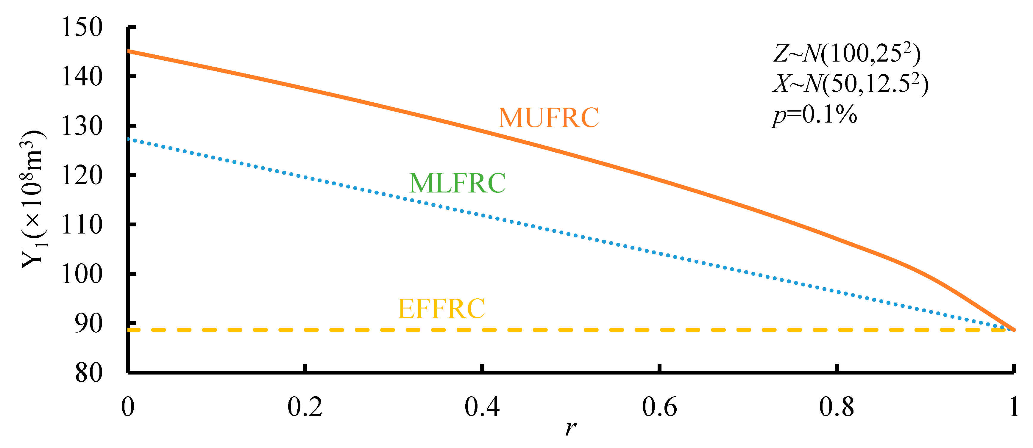
The relationship between the correlation coefficient r and the downstream uncontrolled flood volume was further analyzed as shown in Figure 12 (Assuming that the average of flood volumes for upstream reservoir and the design section were 5 and 10 billion m³, respectively, and the coefficients of variation were both 0.25). The EFFRC method could not reflect the correlation of sub-basins with the assumption that r≡1, so its uncontrolled flood would never alter with r. The flood volume allocated into uncontrolled basin with MLFRC linearly decreased with the increase of r. MUFRC method allocated the most uncontrolled interval flood with a nonlinear decrease, and the greater r was, the faster it decreased. Overall, the smaller r was, the larger the gap among different FRC methods was; while r=1 meant that X and Z were completely linearly correlated, and the FRC scheme (x_p, z_p-x_p) was uniquely determined with the known constant, design flood volume z_p, which was not related to the equal frequency, the probability density, the flood risk and any other factors.

In summary, MUFRC method allocated most flood volume to the downstream uncontrolled sub-basin, followed by MLFRC method, and the least with EFFRC method, so the allocation of the MUFRC brought the greatest risk to the downstream reservoir regulation and flood control.

5. Conclusions

In this study, a novel FRC method, i.e., the most unfavorable flood regional composition (MUFRC) method was proposed to estimate design floods in cascade reservoirs operation period. The case study in Yalong River cascade reservoirs has clarified its practicality. The rationality of proposed method was discussed and compared with different FRC methods. The main conclusions were summarized as follows:

(1) The MUFRC method would further allocate design flood into each sub-basin with the maximum flood prevention risk. The MUFRC method allocated more flood to the uncontrolled inter-basin and presented acceptable stability in sensitivity analysis. Theoretical derivation further confirmed its threat to downstream flood control.

(2) The flood loss would make great difference on MUFRC method. A great value of controllable flood volume

y_{n}^{E}

would indicate strong and stringent flood control security, and made MUFRC method derive unrealistic results. Conversely, MUFRC scheme would not significantly differ from MLFRC method with small

y_{n}^{E}

(3) The most unfavorable design flood of Yalong River basin in cascade reservoir operation period could be derived by MUFRC-allocated flood in sub-basins. Its peak discharge, maximum 1d, 3d and 7d flood volumes has decreased by 36.6%, 36.1%, 33.0% and 28.7%, respectively compared with original designed values. The 4.5 billion m³ flood control storage from upstream reservoir has significantly flattened the design flood even under the most unfavorable condition.

(4) The decrease of design flood would lessen the downstream flood control pressure. Hence, redesigned flood control water levels of JP1 and ET reservoirs could be raised from 1859 m, 1190 m to 1862.39m, 1192.59m, respectively, under the condition of the original flood prevention standards unchanged. The raise of water level led to increases of net head and hydropower generation during the flood season, and could generate 640 million kW·h (+1.82%) more hydropower annually.

Funding

This study was financially supported by the National Natural Science Found of China (U2340205) and National Key Research and Development Plan (2022YFC3202801).

Data Availability Statement

The data presented in this study are available on request from the corresponding author.

Acknowledgments

The authors would like to thank the editor and anonymous reviewers whose comments and suggestions helped to improve the manuscript.

Conflicts of Interest

The authors declare no conflict of interest.

References

Duan, W.; Guo, S.; Wang, J.; et al. Impact of cascaded reservoirs group on flow regime in the middle and lower reaches of the Yangtze River. Water 2016, 8, 218–218. [Google Scholar] [CrossRef]
Guo, S.; Rizwan, M.; Liu, Z.; et al. Design flood estimation methods for cascade reservoirs based on copulas. Water 2018, 10, 560. [Google Scholar] [CrossRef]
Jiang, C.; Xiong, L.; Xu, C.; et al. A river network-based hierarchical model for deriving flood frequency distributions and its application to the upper Yangtze basin. Water Resources Research 2021, 57, 029374–029374. [Google Scholar] [CrossRef]
Lee, D.; Ward, P.J.; Block, P. Attribution of large-scale climate patterns to seasonal peak-flow and prospects for prediction globally. Water Resources Research 2018, 54, 916–938. [Google Scholar] [CrossRef]
Liu, P.; Lin, K.; Wei, X. A two-stage method of quantitative flood risk analysis for reservoir real-time operation using ensemble-based hydrologic forecasts. Stochastic Environmental Research and Risk Assessment 2015, 29, 803–813. [Google Scholar] [CrossRef]
López, J.; Francés, F. Non-stationary flood frequency analysis in continental Spanish rivers, using climate and reservoir indices as external covariates. Hydrology and Earth System Sciences 2013, 17, 3189–3203. [Google Scholar] [CrossRef]
MWR (Ministry of Water Resources). Regulation for calculating design flood of water resources and hydropower projects; Water Resources and Hydropower Press: Beijing, China, 2006. (In Chinese) [Google Scholar]
Nelsen, R. An introduction to copulas, 2nd ed.; Springer-Verlag: New York, 2006. [Google Scholar]
Qi, W.; Liu, J. A non-stationary cost-benefit based bivariate extreme flood estimation approach. Journal of Hydrology 2018, 557, 589–599. [Google Scholar] [CrossRef]
Qi, W. A non-stationary cost-benefit analysis approach for extreme flood estimation to explore the nexus of ‘risk, cost and non-stationarity’. Journal of Hydrology 2017, 554, 128–136. [Google Scholar] [CrossRef]
Rigby, A.; Stasinopoulos, M. Generalized additive models for location, scale and shape. Journal of the Royal Statistical Society Series C: Applied Statistics 2005, 54, 507–554. [Google Scholar] [CrossRef]
Salvadori, G.; Durante, F.; Michele, C.; et al. A multivariate copula-based framework for dealing with hazard scenarios and failure probabilities. Water Resources Research 2016, 52, 3701–3721. [Google Scholar] [CrossRef]
Salvadori, G.; Michele, C. Frequency analysis via copulas: theoretical aspects and applications to hydrological events. Water Resources Research 2004, 40, 12511–12511. [Google Scholar] [CrossRef]
Su, C.; Chen, X. Assessing the effects of reservoirs on extreme flows using nonstationary flood frequency models with the modified reservoir index as a covariate. Advances in Water Resources 2018, 124, 29–40. [Google Scholar] [CrossRef]
Sun, Z.; Zhu, X.; Pan, Y.; et al. Flood risk analysis: progress, challenges and prospect. Journal of Catastrophology 2017, 32, 125–130. (In Chinese) [Google Scholar]
UNDHA (United Nations Department of Humanitarian Affairs). Internationally agreed glossary of basic terms related to disaster management; United Nations Department of Humanitarian Affairs: Geneva, 1992. [Google Scholar]
Volpi, E.; Lazzaro, D.M.; Bertola, M.; et al. Reservoir effects on flood peak discharge at the catchment scale. Water Resources Research 2018, 54, 9623–9636. [Google Scholar] [CrossRef]
Wei, W.; Hong, Y.; Ruby, L.; et al. Nonlinear filtering effects of reservoirs on flood frequency curves at the regional scale. Water Resources Research 2017, 53, 8277–8292. [Google Scholar]
Xie, Y.; Guo, S.; Xiong, L.; et al. Nonstationary design flood estimation in response to climate change, population growth and cascade reservoir regulation. Water 2021, 13, 2687–2687. [Google Scholar] [CrossRef]
Xiong, F.; Guo, S.; Liu, P.; et al. A general framework of design flood estimation for cascade reservoirs in operation period. Journal of Hydrology 2019, 577, 124003. [Google Scholar] [CrossRef]
Xiong, F.; Guo, S.; Yin, J.; et al. Comparative study of flood regional composition methods for design flood estimation in cascade reservoir system. Journal of Hydrology 2020, 590, 125530. [Google Scholar] [CrossRef]
Yin, J.; Guo, S.; Liu, Z.; et al. Uncertainty analysis of bivariate design flood estimation and its impacts on reservoir routing. Water Resources Management 2018, 32, 1795–1809. [Google Scholar] [CrossRef]
Zhang, X.; Liu, P.; Xu, C.; et al. Real-time reservoir flood control operation for cascade reservoirs using a two-stage flood risk analysis method. Journal of Hydrology 2019, 577, 123954–123954. [Google Scholar] [CrossRef]
Zhang, X.; Liu, P.; Chen, J.; et al. Research on the synergistic effect of multi-reservoir flood control capacity by considering the conditional value-at-risk. Advances in Water Science 2022, 33, 298–305. (In Chinese) [Google Scholar]
Zhao, L.; Li, J.; Zhang, T.; et al. Multi-method combined analysis of urban flood risks and its influencing factors under low impact development. Journal of Hydrology 2024, 632, 130927. [Google Scholar] [CrossRef]

Figure 1. Sketch diagram of flood regional composition framework.

Figure 2. Flow chart of design flood estimated by MUFRC method in cascade reservoir operation period.

Figure 3. Sketch location map of cascade reservoirs in the Yalong River.

Figure 4. Cumulative distribution of 7d flood volumes and flood peak fitted by P-III distributions at four (LHK, JP, ET, TZL) cascade reservoirs. P_KS denotes the result of Kolmogorov–Smirnov test.

Figure 5. The AICs for 7d flood volume joint distribution fitted by Copula functions.

Figure 6. The scatters of empirical frequency and theoretical frequency fitted by Copula functions.

Figure 7. The 7d flood volumes of 1000-year design flood for various FRC schemes at TZL section. P_R and Δy_n denote the probability and flood loss indicators for corresponding schemes.

Figure 8. 1000-year design flood hydrographs of TZL section derived by different FRC methods.

Figure 9. Influence of controllable flood volume on 7d flood volume allocation in MUFRC method.

Figure 10. Sensitivity analysis of 7d flood volume regional composition schemes with different sample sizes.

Figure 11. Design floods estimated using Bootstrap method. The filled areas in Figure 11(a~c) present the range of results in all Bootstrap loops and the solid lines present results in Yalong River case study. The ranges in Figure 11(d) are calculated with the difference between the upper and lower boundaries of filled areas in Figure 11 (a~c).

Figure 12. Comparison of flood volumes in uncontrolled sub-basin allocated by various FRC methods under different correlation condition.

Table 1. Basic information of cascade reservoirs in the Yalong River.

Reservoir	LHK	YFG	JP1	JP2	GD	ET	TZL
Drainage area (thousand km²)	65.72	80.88	102.56	102.66	110.12	116.49	127.67
Normal pool level (m)	2865	2094	1880	1646	1330	1200	1015
Flood limit water level (m)	2845.9	-	1859.0	-	-	1190.0	-
Design flood water level (m)	2867	-	1880.5	-	-	1200	1015
Total storage capacity (Billion m³)	107.67	5.13	7.99	0.19	7.60	5.80	0.09
Flood control storage (Billion m³)	2.00	-	1.60	-	-	0.90	-
Installed hydropower capacity (GW)	3.00	1.50	3.60	4.80	2.40	3.30	0.60
Regulation capacity	multi-year	daily	annual	daily	daily	seasonal	daily

Table 2. Comparison of 1000-year design floods of TZL section estimated by different FRC methods.

Design flood	Original value	MUFRC	MLFRC	EFFRC
Q_max (m³/s)	24300	15400 (-36.6%)	15200 (-37.5%)	14800 (-39.3%)
W₁ (10⁸m³)	20.66	13.20 (-36.1%)	13.20 (-36.6%)	12.69 (-38.7%)
W₃ (10⁸m³)	58.39	39.14 (-33.0%)	38.93 (-33.3%)	37.65 (-35.5%)
W₇ (10⁸m³)	118.23	84.22 (-28.7%)	83.06 (-29.7%)	81.20 (-31.3%)

Disclaimer/Publisher’s Note: The statements, opinions and data contained in all publications are solely those of the individual author(s) and contributor(s) and not of MDPI and/or the editor(s). MDPI and/or the editor(s) disclaim responsibility for any injury to people or property resulting from any ideas, methods, instructions or products referred to in the content.

© 2024 by the authors. Licensee MDPI, Basel, Switzerland. This article is an open access article distributed under the terms and conditions of the Creative Commons Attribution (CC BY) license (http://creativecommons.org/licenses/by/4.0/).

Copyright: This open access article is published under a Creative Commons CC BY 4.0 license, which permit the free download, distribution, and reuse, provided that the author and preprint are cited in any reuse.

MDPI Initiatives

Important Links

Choose an area of interest and we will send you notifications of new preprints at your preferred frequency.

Disclaimer

A Novel Flood Regional Composition Method for Design Flood Estimation in the Cascade Reservoirs

Abstract