Preprint
Article

Brain-Inspired Sparse Training in MLP and Transformers with Network Science Modeling via Cannistraci-Hebb Soft Rule

Altmetrics

Downloads

231

Views

223

Comments

0

Submitted:

14 June 2024

Posted:

17 June 2024

You are already at the latest version

Alerts
Abstract
Dynamic sparse training is an effective strategy to alleviate the training and inference demands of artificial neural networks. However, current sparse training methods face a challenge in achieving high levels of sparsity while maintaining performance comparable to that of their fully connected counterparts. The Cannistraci-Hebb training (CHT) method produces an ultra-sparse advantage compared to fully connected training in various tasks by using a gradient-free link regrowth method, which relies solely on the network topology. However, its rigid selection based on link prediction scores may lead to epitopological local minima, especially at the beginning of the training process when the network topology might be noisy and unreliable. In this article, we introduce the Cannistraci-Hebb training soft rule (CHTs), which applies a flexible approach to both the removal and regrowth of links during training, fostering a balance between exploring and exploiting network topology. Additionally, we investigate the network topology initialization using several approaches, including the bipartite scale-free and bipartite small-world network models. Empirical results show that CHTs can surpass the performance of fully connected networks with MLP architecture by using only 1% of the connections (99% sparsity) on the MNIST, EMNIST, and Fashion MNIST datasets and can provide remarkable results with only 0.1% of the links (99.9% sparsity). In some MLPs for image classification tasks, CHTs can reduce the active neuron network size to 20% of the original nodes (neurons), demonstrating a remarkable ability to generalize better than fully connected architectures, reducing the entire model size. This represents a relevant result for dynamic sparse training. Finally, we present evidence from larger network models such as Transformers, with 10% of the connections (90% sparsity), where CHTs outperform other prevalent dynamic sparse training methods in machine translation tasks.
Keywords: 
Subject: Computer Science and Mathematics  -   Artificial Intelligence and Machine Learning

1. Introduction

Artificial neural networks (ANNs) have spurred significant advancements in various fields, such as natural language processing, computer vision, and deep reinforcement learning. The most common ANNs include several fully connected (FC) layers: for instance, FC layers represent a significant portion of recent large language models’ parameters [1,2]. This dense connectivity poses major challenges during both the training and the deployment phases of the models. Unlike these ANNs, the brain’s neural networks inherently exhibit sparse connectivity [3,4]. This natural design in the brain, which leverages sparsity, suggests a model where the number of connections does not need to scale quadratically with the number of neurons. This could alleviate the computational constraints, thus allowing for more scalable network architectures.
Dynamic sparse training (DST) [5,6,7,8,9] has emerged as a promising approach to reduce the computational and memory overheads of training deep neural networks while maintaining or even enhancing model performance. Unlike Pruning methods [10,11,12], DST starts with an already sparse initialized network and maintains this sparsity throughout the training process. The prevalent DST methods will evolve the network topology during the training stage by applying removal-and-regrown iterations: removing a proportion of connections and regrowing the network with an equivalent number of links.
Apart from some detailed distinctions, the primary innovation in this field revolves around developing the regrowth criterion. A notable advancement is the gradient-free regrowth method introduced by the Cannistraci-Hebb training (CHT) [9]. This method draws inspiration from a brain-inspired network science theory [13,14,15,16,17] and has been demonstrated to produce a significant advantage in training ultra-sparse (1% or lower network connectivity) ANNs, outperforming fully connected networks across various tasks. Despite these innovations, CHT faces notable challenges, particularly its tendency to become trapped in epitopological local minima, which can significantly hinder the progress of epitopological exploration. The term epitopological means literally “new topology" and refers to epitopological learning [9], which is a field of network science and complex network intelligence that studies how to implement learning on complex networks by changing the shape of their connectivity structure (epitopological plasticity).
In this article, we introduce the Cannistraci-Hebb Training soft rule (CHTs). CHTs selects links based on scores sampled from removal and regrowth metrics by Binomial distribution. Additionally, we explore diverse methods for sparse topological initialization, including the application of two network science bipartite models. We enhance the performance of the Bipartite Scale-Free network model (BSF) [9] through a strategy that aligns by degree sorting the input and output degree of neurons in the same layer. Moreover, we investigate the performance of the Bipartite Small-World (BSW) model [9] by tuning its β parameter (for random connectivity rewiring) to achieve optimal performance and delve into the underlying reasons for its effectiveness.
To evaluate the effectiveness of CHTs, we conduct experiments using MLPs on image classification tasks (MNIST [18], EMNIST [19], and Fashion MNIST [20]) and Transformers [21] on machine translation tasks (Multi30k en-de [22], IWSLT14 en-de [23], and WMT17 en-de [24]). Our empirical findings showcase that CHTs: (1) can outperform fully connected networks with merely 1% of the connections (99% sparsity) in MLPs on the image classification task; (2) can provide remarkable results using only 0.1% links (99.9% sparsity) in MLPs on the image classification task; (3) can surpass other dynamic sparse training methods with 10% of the connections (90% sparsity) in Transformer on machine translation tasks. It is important to note that the link regrowth step in CHTs solely depends on the network’s topology, without considering gradient or input data, which emphasizes the relevance of the network shape intelligence (NSI). NSI is the intelligence displayed by any topological network automata such as CHT and CHTs to perform valid (significantly more than random) connectivity predictions by only processing the input knowledge associated with the local topological network organization [9,25]. Additionally, we observed that topologies initialized with the BSW model with around β = 0.25 consistently yield the best performance across all tasks because this network topology initialization facilitates the epitopological prediction of links via CHT and CHTs.

2. Related Works

2.1. Dynamic Sparse Training

Dynamic sparse training is a subset of sparse training methodologies. Unlike the static sparse training (also known as pruning at initialization) methods [26,27,28,29], dynamic sparse training allows for the evolution of network topology during the training process. The pioneering method in this field was Sparse Evolutionary Training (SET) [5], which removes links based on the magnitude of their weights and regrows new links randomly. Subsequent developments have sought to refine and expand upon this concept of dynamic topological evolution. One such advancement was proposed by DeepR [30], a method that adjusts network connections based on stochastic gradient updates combined with a Bayesian-inspired update rule. Another significant contribution is the RigL [7], which leverages the gradient information of non-existing links to guide the regrowth of new connections during training. MEST [8] utilizes both gradient and weight magnitude information to selectively remove and randomly regrow new links, which is the same as SET. In addition, it introduces an EM&S strategy that allows the model training with a larger density and finally convergence to the desired density. The Top-KAST [6] method maintains constant sparsity throughout training by selecting the top K parameters based on parameter magnitude at each training step and applying gradients to a broader subset B, where B A . To avoid settling on a suboptimal sparse subset, Top-KAST also introduces an auxiliary exploration loss that encourages ongoing adaptation of the mask. Additionally, sRigL [31] adapts the principles of RigL to semi-structured sparsity, facilitating the training of vision models from scratch with actual speed-ups during training phases. Despite these advancements, the state-of-the-art method remains RigL-based, yet it is not fully sparse in backpropagation, necessitating the computation of gradients for non-existing links. Addressing this limitation, Zhang et al. [9] propose CHT, a dynamic sparse training methodology that adopts a gradient-free regrowth strategy that relies solely on topological information (network shape intelligence), achieving an ultra-sparse configuration that surpasses fully connected networks in some tasks.

2.2. Cannistraci-Hebb Theory and Network Shape Intelligence

As the SOTA gradient-free link regrown method, CHT [9] originates from a brain-inspired network science theory. Drawn from neurobiology, Hebbian learning was introduced in 1949 [32] and can be summarized in the axiom: “neurons that fire together wire together.” This could be interpreted in two ways: changing the synaptic weights (weight plasticity) and changing the shape of synaptic connectivity [13,14,15,16,17]. The latter is also called epitopological plasticity [13] because plasticity means “to change shape,” and epitopological means “via a new topology.” Epitopological Learning (EL) [14,15,16] is derived from this second interpretation of Hebbian learning and studies how to implement learning on networks by changing the shape of their connectivity structure. One way to implement EL is via link prediction, which predicts the existence and likelihood of each nonobserved link in a network. In this study, we adopt CH3-L3 [33] as link predictor to regrow the new links during the DST process. CH3-L3 is one of the best and most robust performing network automata which is inside Cannistraci-Hebb (CH) theory [33] that can automatically evolve the network topology with the given structure. The rationale is that, in any complex network with local-community organization, the cohort of nodes tends to be co-activated (fire together) and to learn by forming new connections between them (wire together) because they are topologically isolated in the same local community [33]. This minimization of the external links induces a topological isolation of the local community, which is equivalent to forming a barrier around the local community. The external barrier is fundamental to maintaining and reinforcing the signaling in the local community, inducing the formation of new links that participate in epitopological learning and plasticity. The mathematical formula of CH3-L3 and its explanation is illustrated in Figure 1.

2.3. Bipartite Scale-Free model and Bipartite Small-World model

In artificial neural networks (ANNs), fully connected networks are inherently bipartite. This article explores initializing bipartite networks using models from network science. The Bipartite Scale-Free (BSF) [9] network model extends the concept of scale-freeness to bipartite structures, making them suitable for dynamic sparse training. Initially, the BSF model generates a monopartite Barabási-Albert (BA) model [34], a well-established method for creating scale-free networks in which the degree distribution follows a power law ( γ = 2.76 in Figure 2). Following the creation of the BA model, the BSF approach removes any connections between nodes of the same type (neuron in the same layer) and rewires these connections to nodes of the opposite type (neuron in the opposite layer). This rewiring is done while maintaining the degree of each node constant to preserve the power-law exponent γ .
The Bipartite Small-World (BSW) network model [9] is designed to incorporate small-world properties and high clustering coefficient into bipartite networks. Initially, the model constructs a regular ring lattice and assigns two distinct types of nodes to it. Each node is connected by an equal number of links to the nearest nodes of the opposite type, fostering high clustering but lacking the small-world property. Similar to the Watts-Strogatz model (WS) [35], the BSW model introduces a rewiring parameter, β , which represents the percentage of links randomly removed and then rewired within the network. At β = 1 , the model transitions into an Erdős-Rényi model [36], exhibiting small-world properties but without high clustering coefficient. Figure 2 illustrates example adjacency matrices for the BSF model and the BSW models with varying β values.

2.4. Correlated Sparse Topological Initialization

Correlated Sparse Topological Initialization (CSTI) is a physical-informed topological initialization. CSTI generates the adjacency matrix by computing the Pearson correlation between each input feature across the calibration dataset and then selects the predetermined number of links, calculated based on the desired sparsity level, as the existing connections. CSTI performs remarkably better when the layer can directly receive input information. However, for layers that cannot receive inputs directly, it cannot capture the correlations from the start since the model is initialized randomly, as in the case of the Transformer. Therefore, in this article, we aim to address this issue by investigating different network models to initialize the topology, with the goal of improving the performance for cases where CSTI cannot be directly applied.

3. Network Science Modeling Via Cannistraci-Hebb Training Soft Rule

In this section, we detail our principal innovations that incorporate network science theory to enhance dynamic sparse training. The entire steps for CHTs are illustrated in Figure 1.

3.1. Sparse Topological Initialization with Network Science Models

As demonstrated in CHT [9], the final trained model converges to form an ultra-small-world network, integrating both scale-free and small-world properties. This raises the question: what if the network is initialized directly with these characteristics? In this section, we delve deeper into the utility of network science models to enhance the topological initialization of dynamic sparse training, aiming for a comprehensive understanding and analysis.

3.1.1. Equal Partition and Neuron Resorting to Enhance BSF Initialization

As indicated in SET and CHT [5,9], trained sparse models typically converge to a scale-free network. This suggests that initiating the network with a scale-free structure might initially enhance performance. However, starting directly with a Bipartite Scale-Free model (BSF, power-law exponent γ = 2.76 ) does not yield effective results. Upon deeper examination, two potential reasons emerge:
  • The BSF model generates hub nodes randomly. However, This random assignment of hub nodes to less significant inputs leads to a less effective initialization, which is particularly detrimental in CHT, which merely utilizes the topology information to regrow new links.
  • As demonstrated in CHT, in the final network, the hub nodes of one layer’s output should correspond to the input layer of the subsequent layer, which means the hub nodes should have a high degree on both sides of the layer. However, the BSF model’s random selection disrupts this correspondence, significantly reducing the number of Credit Assignment Paths (CAP) [9] in the model. CAP is defined as the chain of the transformation from input to output, which counts the number of links that go through the hub nodes in the middle layers.
To address these issues, we propose two solutions:
  • Equal Partitioning of the First Layer: We begin by generating a BSF model, then rewire the connections from the input layer to the first hidden layer. While keeping the out-degrees of the output neurons fixed, we randomly sample new connections to the input neurons until each of the input neurons’ in-degrees reaches the input layer’s average in-degree. This approach ensures all input neurons are assigned equal importance while maintaining the power-law degree distribution of output neurons.
  • Resorting Middle Layer Neurons: Given the mismatch in hub nodes between consecutive layers, we suggest permuting the neurons between the output of one layer and the input of the next, based on their degree. A higher degree in an output neuron increases the likelihood of connecting to a high-degree input neuron in the subsequent layer, thus enhancing the number of CAPs.

3.1.2. Why Is the BSW Model the Best Network Science-Based Initialization Approach?

Figure 4c demonstrates that the Bipartite Small-World (BSW) model with β =0.25 consistently outperforms the BSF model across basic datasets even with the adjustment described above. The BSW model, characterized by its small world properties, ensures both clustering and small average path length. The high clustering, which is not present in the BSF model, facilitates a higher probability for seed nodes to share common neighbors along L3 paths (path length of three), increasing the likelihood of CH3-L3 score to produce valid predictions at the start of the training. Conversely, the BSF model’s preferential attachment nature results in the emergence of hub nodes and a negligible clustering structure, which implies that common neighbors along L3 paths are less likely to occur in the BSF network, increasing the likelihood of CH3-L3 zero score prediction (absence of relevant topological prediction) for missing links. Additionally, starting from a scale-free BSF model will probably lead to the epitopological local minima (ELM, Definition 1). It enhances the predictability for CH3-L3 [33], but restricts its ability to escape this ELM. Overall, the BSW model with a β of approximately 0.25 consistently offers superior performance compared to other network science models.

3.2. Cannistraci-Hebb Soft Removal and Regrown

Definition 1.
Epitopological local minima.
In the context of dynamic sparse training methods, we define an epitopological local minima (ELM) as a state where the sets of removed links and regrown links exhibit a significant overlap. Let A t be the set of existing links in the network at the training step t. Let A ˜ t be the set of removal links and A t * be the set of regrown links. The overlap set between removed and regrown links at step t can be quantified as O t = A ˜ t A t * . An ELM occurs if the size of O t at step t is significantly large compared to the size of A t * , indicating a high probability of the same links being removed and regrown repeatedly throughout the subsequent training steps. This can be formally represented as | O t | | A t * | θ , where θ is a predefined threshold close to 1, indicating strong overlap. This definition is essential for the understanding of CHT, as evidenced by the article [9] indicating that the overlap rate between removed and regrown links becomes significantly high within just a few epochs, leading to rapid topological convergence towards the ELM. Previously, CHT implements a topological early stop strategy to avoid predicting the same links iteratively. However, it will stop the topological exploration very fast and potentially trap the model within the ELM. We propose the Cannistraci-Hebb soft rule for both the removal and regrowth phases to facilitate CHT to escape from the ELM.
In this article, we adopt a probabilistic approach where the process of link removal and regrowth can be viewed as sampling from a { 0 , 1 } binomial distribution, with the score assigned by either removal metrics or link prediction scores, introducing a "soft sampling" mechanism. In this setup, each mask value is not rigidly determined by the scores but allows for selecting (with lower probability) low-score links as new links, facilitating the escape from the epitopological local minima (ELM).

3.2.1. Soft Link Removal Alternating from Weight Magnitude and Relative Importance

We illustrate link removal part of CHTs in Figure 1b1,b2. We employ two methods, Weight Magnitude (WM) | W | and Relative Importance (RI) [12], to remove the connections during dynamic sparse training:
RI i j = | W i j | | W * j | + | W i j | | W i * |
As illustrated in Equation 1, RI assesses connections by normalizing the absolute weight of links that share the same input or output neurons. This method does not require calibration data and can perform comparably to the baseline post-training pruning methods like sparsegpt [11] and wanda [37]. Generally, Weight Magnitude (WM) and RI are straightforward, effective, and quick to implement in DST for link removal but give different directions for network percolation. WM prioritizes links with higher weight magnitudes, leading to rapid network percolation, whereas RI inherently values links connected to lower-degree nodes, thus maintaining a higher active neuron post-percolation (ANP) rate. The ANP rate is the ratio of the number of active neurons after training compared to the original number of neurons before training. These methods are equally valid but cater to different scenarios. For instance, using RI significantly improves results on the Fashion MNIST dataset compared to WM, whereas WM performs better on the MNIST and EMNIST datasets.
In the initial training stage, both WM and RI lack significance due to the model’s underdevelopment. Therefore, instead of selecting the top values of WM and RI, we sample from a Binomial distribution guided by the importance score computed by the removal metrics. The formula for selecting links to remove is presented in Equation 2. We utilize two parameters to adjust the formulation of the importance score S that determines which links are removed.
S i j = | W i j | / 2 α + ( 1 α ) | W i * | + | W i j | / 2 α + ( 1 α ) | W * j | δ 1 δ
The parameter α determines the removal method. Specifically, when α = 0 , the formula relies on the RI, and when α = 1 , it utilizes WM. For the purposes of this study, we limit our exploration to these settings and do not investigate intermediate values of α , leaving the possibility of hybrid strategies for future research. Additionally, the parameter δ controls the temperature of the sampling process. A value of δ = 0 results in uniformly random sampling. In contrast, as δ increases towards 1, the sampling becomes more deterministic. In this article, we implement a soft removal strategy that linearly increases δ from 0.5 to 0.75, reflecting a gradual transition strategy from exploration to exploitation as the model converges, thus increasing the likelihood of retaining more significant links within the network as training progresses.

3.2.2. Network Percolation and Extension to Transformer

We have adapted network percolation [9,38] to suit the architecture of the Transformer after link removal. The underlying concept involves identifying inactive neurons, which we define as those lacking connections on one or both sides of a neuron layer. Such neurons disrupt the flow of information during forward propagation or backpropagation. In addition, Layer-wise computation of the CH3-L3 score further implies that neurons without connections on one side are unlikely to form connections in the future. Therefore, network percolation becomes essential to optimize the use of remaining links.
As shown in Figure 1, network percolation encompasses two primary processes: c1) inactive neuron removal to remove the neurons that lack connections on one or both sides; c2) incomplete path adjustment to remove the incomplete paths where links connect to the inactive neurons after c1). Typically applied in simpler continuous layers like those in an MLP, network percolation requires modification for more complex structures. For example, within the Transformer’s self-attention module, the outputs of the query and key layers undergo a dot product operation. It necessitates percolation in these layers to examine the activity of the neurons in both output layers at the same position. Similar interventions are necessary in the up_proj and gate_proj layers of the MLP module in the LLaMA model family [1,39].

3.2.3. Soft Link Regrown Based on CH3-L3 Network Automata

CH3-L3 is recognized as the most effective network automaton within the Cannsitraci-Hebb theory [33]. CHT traditionally uses the top-k value predicted by CH3-L3 to determine which links to regrow, While this ‘rigid’ strategy works well in case the network topology is reliable (as in link prediction on well-observed real networks), at the start of the training process the network topologies is noised and unreliable therefore adopting a rigid top-k prioritization of the new links to grow might lead to stagnation in an ELM. To mitigate this limitation, we introduce a soft rule for sampling new links using also the Binomial distribution. We have modified the original CH3-L3 equation as shown in Equation 3:
CH 3 L 3 s ( u , v ) = z 1 , z 2 L 3 1 d e z 1 * * d e z 2 * δ 1 δ
In this equation, u and v represent the seed nodes, while z 1 and z 2 are common neighbors [33] on the L3 path. The term d e i * denotes the number of external local community links (eLCL) of node i, and is incremented by 1 by default to prevent e L C L from becoming zero, as depicted in Figure 1d2. Similarly to the link removal process, we use the parameter δ to adjust the sampling temperature. As δ approaches zero (random strategy), the model randomly regrows new links, enhancing exploration of the topology. As δ =0.5, the model will sample with the original CH3-L3 score by Binomial distribution. Conversely, as δ nears one, the model strictly follows the CH3-L3 score to regrow links, thereby focusing on exploiting the existing topological structure. In this study, we refer to α =0 as a random regrown strategy and α = 0.5 as the CH3-L3-soft, while strictly adhering to the CH3-L3 score is termed the CH3-L3-rigid. An illustration of how to compute CH3-L3s is shown in Figure 1.

4. Experiments

4.1. Setup

We conduct experiments using MLPs for image classification tasks on the MNIST [18], Fashion MNIST [20], and EMNIST [19] datasets, and Transformers for machine translation tasks on the Multi30k en-de [22], IWSLT14 en-de [23], and WMT17 en-de [24] datasets. For the MLPs, we initiate with a learning rate of 0.025 and apply a linear decay strategy down to 2.5 × 10 4 . The architecture of the MLP is 784 1568 1568 1568 10 . Dynamic sparse training (DST) is implemented for all but the final layer of the MLP since the neurons in the output layer might be disconnected because of the ultra-sparsity. For the Transformer, we train the model using the iterative noam (inoam) [40] technique, which contains a brief warmup period after each iteration to accommodate the reset states of the new links. This warmup period is typically 20 steps, guided by the exponential decay rate β used in the Adam optimizer. We apply DST to all linear layers except the embedding and the final linear layer. Experiments were conducted on one A100 GPU. The comprehensive configurations of the MLP and Transformer models are provided in Table A1 and Table A2.

4.2. Baseline Methods

We compare our method with widely used dynamic sparse training methods: SET [5], RigL [7], and CHT [9]. Each of these methods removes connections based on the magnitude of their weights. SET, the baseline method, randomly regrows new links. RigL regrows links based on the gradient of non-existing links and gradually incorporates a function to decrease the proportion of connections that are updated over time. CHT, currently considered a state-of-the-art (SOTA) gradient-free (only topological-based) method, regrows links rigidly based on CH3-L3 scores.

4.3. Results on MLP

4.3.1. Ablation Test

Using MLP, we conduct an ablation study on each component proposed within the CHTs framework to determine the most effective implementation to apply next for the Transformer model. As illustrated in Figure 3a, to enhance DST initialized with a Bipartite Scale-Free (BSF) model, we proposed two strategies. The results indicate that resorting neurons based on their degree generally improves performance, suggesting that increasing credit assignment paths at initialization can boost DST efficiency. Figure 3b compares the topologies initialized with the Bipartite Small-World (BSW) model at different values of β , clearly indicating that β = 0.25 yields the best results. Figure 3c,d assess the link removal and link regrowth methods, respectively, concluding that the weight magnitude soft (WM-soft) and CH3-L3-soft methods outperform all others. We consider the best settings showcased in these results to decide the CHTs strategy for training Transformers.

4.3.2. Main Results

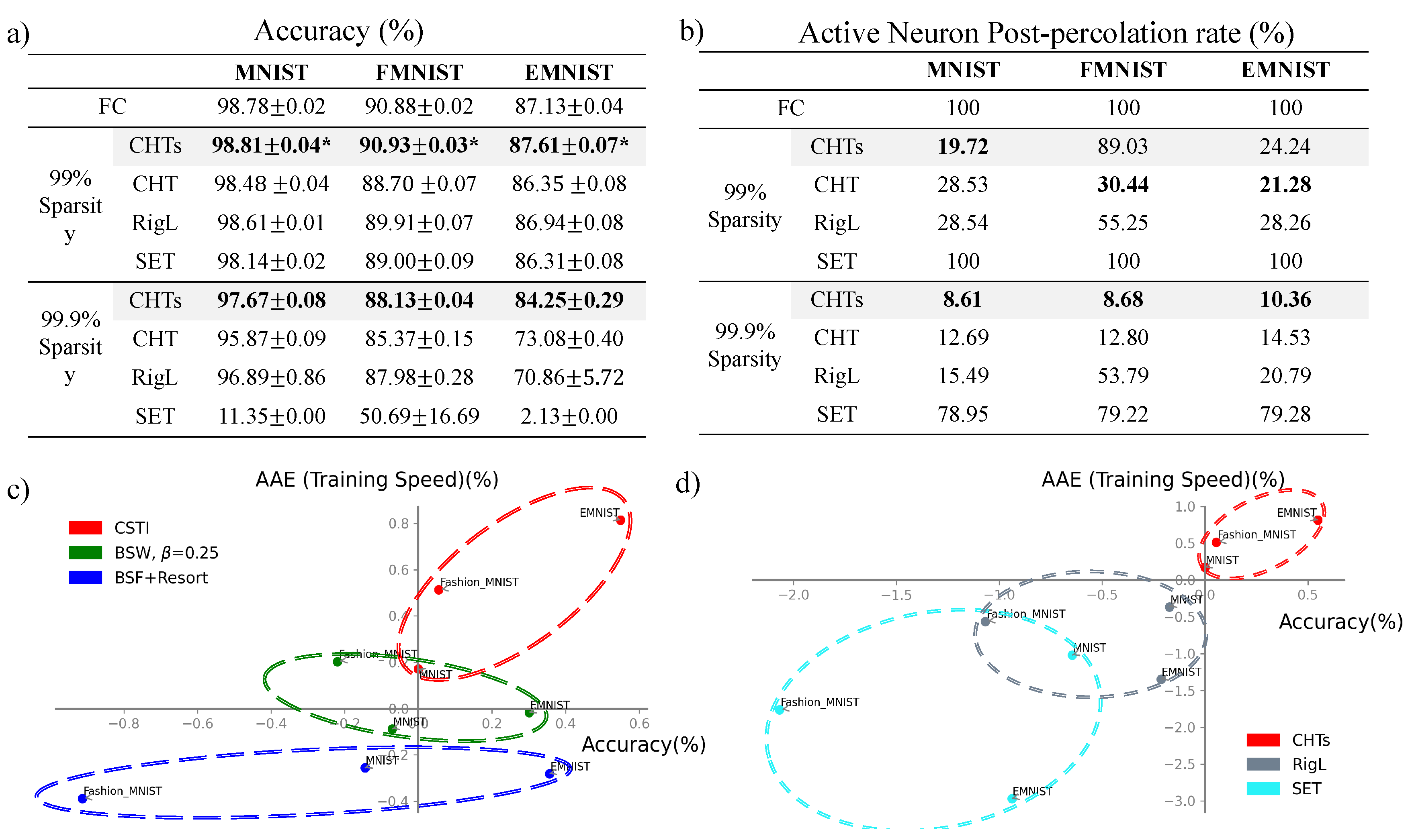
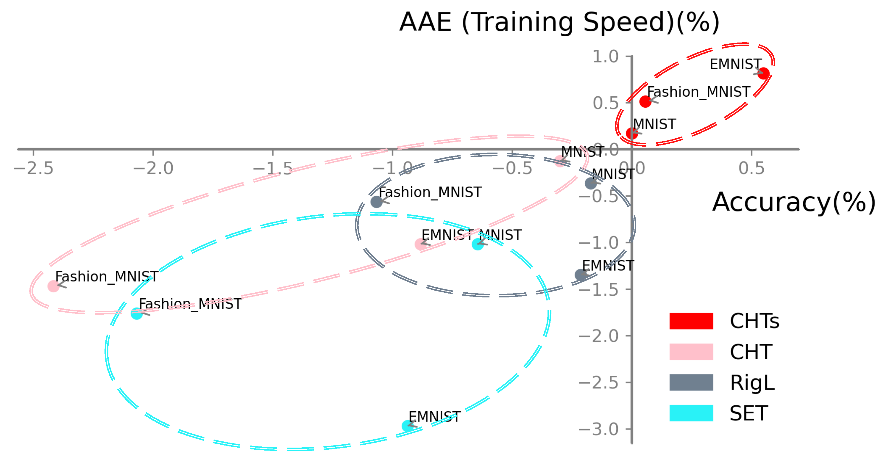
In the MLP evaluation, we aim to assess the fundamental capacity of DST methods to train the fully connected module, which is common across many ANNs. Figure 4a displays the ultimate performance of DST methods compared to their fully connected counterparts across three basic datasets. The DST methods are tested at 99% and 99.9% sparsity levels. Notably, CHTs outperforms other DST methods in both sparsity scenarios and achieves a substantial advantage over the fully connected network at 99% sparsity. In Figure 4b, we present the active neuron post-percolation rate (ANP) for each method, corresponding to the performance metrics in Figure 4a. It is evident that CHT consistently facilitates the highest percolation rate, demonstrating its robust intuitive design. However, CHTs adaptively percolates the network more effectively. Notably, for the Fashion MNIST dataset, the best performance is achieved using the RI-soft removal method, which inherently maximizes node retention, hence maintaining a high ANP for CHTs. Figure 4d compares the performance ratios of DST methods relative to their fully connected counterparts in terms of area across epochs (AAE) [9], indicating learning speed, and accuracy. The reference point is the fully connected network. Here, CHTs consistently exhibits a significant ultra-sparse advantage in both learning speed and accuracy across all datasets, while the other DST methods cannot. We also demonstrate the performance of CHTs and CHT in Appendix Figure 4c and Figure 5. laterally compares all topological initializations. Although initializing with Correlated Sparse Topological Initialization (CSTI) [9] remains the best, it requires calibration data to calculate input correlations, making it impractical for layers that do not directly receive input signals, such as most modules in Transformers. When comparing BSW with β = 0.25 and BSF combined with resorting neurons, which are depicted in Figure 3a,b as the best in internal checks, BSW with β = 0.25 generally performs better.

4.4. Results on Transformer

We assess the Transformer’s performance on a classic machine translation task across three datasets. We take the best performance of the model on the validation set and report the BLEU on the test set. Beam search, with a beam size of 2, is employed to optimize the evaluation process. In our evaluation, CHTs configures the topology of each layer using the BSW model with β = 0.25 , employs WM-soft for link removal, and regrows new links using CH3-L3-soft. Additionally, we apply an adjusted network percolation technique to the Transformer, as detailed in Section 3.2.2. The findings, presented in Table 1, demonstrate that with 90% sparsity, CHTs surpasses other DST methods in performance while the decrease in performance with respect to fully connected training is contained.

5. Conclusion and Discussion

In this paper, we introduce the Cannsitraci-Hebb training soft rule (CHTs) for topological-driven dynamic sparse training, exploring the integration of network science models such as the Bipartite Scale-Free and Bipartite Small-World models. These models provide an initial topological structure, embedding certain topological features from the outset. Our novel approach utilizes a soft rule for network connectivity, where the selection isn’t strictly based on the highest scores of importance or link prediction from CH3-L3 network automata. Instead, we employ a binomial distribution for sampling, which offers a more flexible strategy. Empirically, CHTs demonstrate a remarkable ability to achieve ultra-sparse configurations—up to 99% sparsity in MLPs for image classification—surpassing fully connected networks. We offer evidence that CHTs offers interesting performance even on MLPs at 99.9% sparsity. Moreover, when applied to Transformers at 90% sparsity, CHTs outperform other leading dynamic sparse training methods like RigL and SET. Notably, the regrowth process under CHTs does not rely on gradients. In contrast to RigL, which depends on inputs, topology, weights, and activation functions for predicting new connections, CHTs regrowth is merely network topology-driven. Finally, in some MLP tasks for image classification, CHTs can reduce the active neuron network size to 20% of the original nodes (neurons), demonstrating a remarkable ability to generalize better than fully connected architectures, reducing the entire model size. This represents a relevant result for DST. We describe the limitations of this study and future works in Appendix A.

Appendix A. Limitation and Future Work

A potential limitation of this work is that the hardware required to accelerate sparse training with unstructured sparsity has not yet become widely adopted. Consequently, this article does not present a direct comparison of training speeds with those of fully connected networks. However, several leading companies [41] have already released devices that support unstructured sparsity in training. Another limitation concerns the computation of CH3-L3, which is O ( N × d 3 ) [9], where N represents the number of nodes and d is the maximum degree of nodes in the network. As the network density increases, the execution time becomes prohibitively long. Addressing this issue will be a focus of our future studies.
For future work, we aim to develop methods for automatically determining the temperature for soft sampling at each epoch, guided by the topological features of each layer. This could enable each layer to learn its specific topological rules autonomously. Additionally, we plan to test CHTs in large language models to evaluate their performance in scenarios with several FC layers.

Appendix B. Broader Impact

In this work, we introduce a novel methodology for dynamic sparse training aimed at enhancing the efficiency of AI model training. This advancement holds potential societal benefits by increasing interest in more efficient AI practices. However, the widespread availability of advanced artificial neural networks, particularly large language models (LLMs), also presents risks of misuse. It is essential to carefully consider and manage these factors to maximize benefits and minimize risks.

Appendix C. Comparative Analysis of CHTs and SST Using CHTs’ Topology
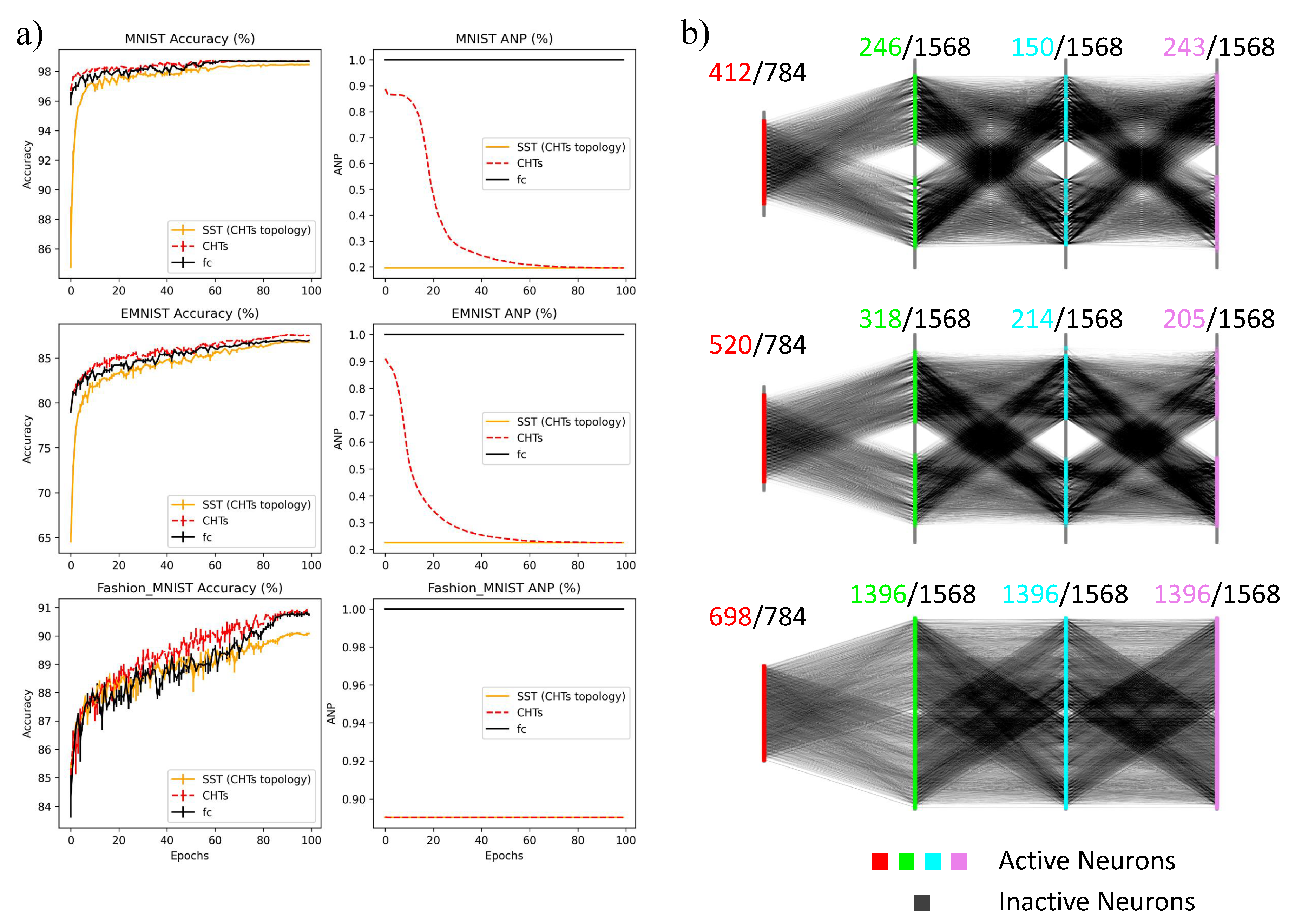
In this section, we address the hypothesis that it is not static topology but dynamic topological growth that steers the gradient directions during ‘online’ topological evolution.
To test this, we retrain the final MLP topology developed through CHTs on 3 basic datasets using static sparse training (SST) and then compare it with the results of CHTs and fully connected architectures. Guided by the Lottery Ticket Hypothesis (LTH) [42], we initialize the weights for SST identically to those used in CHTs. As depicted in Figure A1a, the comparisons across three datasets reveal that SST (CHT topology, Figure A1b) does not perform as well as CHTs. These findings validate our hypothesis.
Figure A1. Performance Comparison of CHTs, static sparse training (SST) Using CHTs’ Final Topology, and Fully Connected Networks. a) evaluates the performance and the Active Neuron Post-percolation Rate (ANP) of CHTs, SST (CHTs topology), and fully connected networks (fc) across the MNIST, EMNIST, and Fashion MNIST datasets. b) presents the final topology developed through CHTs, which serves as the initial topology for SST.
Preprints 109312 g0a1
Table A1. Hyperparameters of MLP on Image Classification Tasks.
Hyper-parameter MLP
Hidden Dimension 1568
# Hidden layers 3
Batch Size 32
Training Epochs 100
LR Decay Method Linear
Learning Rate 0.025
Update Interval (for DST) 1
Table A2. Hyperparameters of Transformer on Machine Translation Tasks.
Hyper-parameter Multi30k IWSLT14 WMT17
Embedding Dimension 512 512 512
Feed-forward Dimension 1024 2048 2048
Batch Size 1024 tokens 10240 tokens 12000 tokens
Training Steps 20000 20000 80000
Dropout 0.1 0.1 0.1
Attention Dropout 0.1 0.1 0.1
Max Gradient Norm 0 0 0
Warmup Steps 3000 6000 8000
Decay Method inoam inoam inoam
Label Smoothing 0.1 0.1 0.1
Layer Number 6 6 6
Head Number 8 8 8
Learning Rate 0.25 2 2
Update Interval (for DST) 200 100 100

References

  1. Touvron, H.; Lavril, T.; Izacard, G.; Martinet, X.; Lachaux, M.A.; Lacroix, T.; Rozière, B.; Goyal, N.; Hambro, E.; Azhar, F.; others. Llama: Open and efficient foundation language models. arXiv preprint arXiv:2302.13971 2023, arXiv:2302.13971 2023. [Google Scholar]
  2. Zhang, S.; Roller, S.; Goyal, N.; Artetxe, M.; Chen, M.; Chen, S.; Dewan, C.; Diab, M.; Li, X.; Lin, X.V.; others. Opt: Open pre-trained transformer language models. arXiv preprint arXiv:2205.01068 2022, arXiv:2205.01068 2022. [Google Scholar]
  3. Drachman, D.A. Do we have brain to spare?, 2005.
  4. Walsh, C.A. Peter Huttenlocher (1931–2013). Nature 2013, 502, 172–172. [Google Scholar] [CrossRef] [PubMed]
  5. Mocanu, D.C.; Mocanu, E.; Stone, P.; Nguyen, P.H.; Gibescu, M.; Liotta, A. Scalable training of artificial neural networks with adaptive sparse connectivity inspired by network science. Nature communications 2018, 9, 1–12. [Google Scholar] [CrossRef]
  6. Jayakumar, S.; Pascanu, R.; Rae, J.; Osindero, S.; Elsen, E. Top-kast: Top-k always sparse training. Advances in Neural Information Processing Systems 2020, 33, 20744–20754. [Google Scholar]
  7. Evci, U.; Gale, T.; Menick, J.; Castro, P.S.; Elsen, E. Rigging the Lottery: Making All Tickets Winners. Proceedings of the 37th International Conference on Machine Learning, ICML 2020, 13-18 July 2020, Virtual Event. PMLR, 2020, Vol. 119, <italic>Proceedings of Machine Learning Research</italic>, pp. 2943–2952.
  8. Yuan, G.; Ma, X.; Niu, W.; Li, Z.; Kong, Z.; Liu, N.; Gong, Y.; Zhan, Z.; He, C.; Jin, Q.; others. Mest: Accurate and fast memory-economic sparse training framework on the edge. Advances in Neural Information Processing Systems 2021, 34, 20838–20850. [Google Scholar]
  9. Zhang, Y.; Zhao, J.; Wu, W.; Muscoloni, A.; Cannistraci, C.V. Epitopological learning and Cannistraci-Hebb network shape intelligence brain-inspired theory for ultra-sparse advantage in deep learning. The Twelfth International Conference on Learning Representations, 2024.
  10. Han, S.; Mao, H.; Dally, W.J. Deep Compression: Compressing Deep Neural Network with Pruning, Trained Quantization and Huffman Coding. 4th International Conference on Learning Representations, ICLR 2016, San Juan, Puerto Rico, May 2-4, 2016, Conference Track Proceedings; Bengio, Y.; LeCun, Y., Eds., 2016.
  11. Frantar, E.; Alistarh, D. Massive language models can be accurately pruned in one-shot. arXiv preprint arXiv:2301.00774, arXiv:2301.00774 2023.
  12. Zhang, Y.; Bai, H.; Lin, H.; Zhao, J.; Hou, L.; Cannistraci, C.V. Plug-and-Play: An Efficient Post-training Pruning Method for Large Language Models. The Twelfth International Conference on Learning Representations, 2024.
  13. Cannistraci, C.V.; Alanis-Lobato, G.; Ravasi, T. From link-prediction in brain connectomes and protein interactomes to the local-community-paradigm in complex networks. Scientific reports 2013, 3, 1613. [Google Scholar] [CrossRef]
  14. Daminelli, S.; Thomas, J.M.; Durán, C.; Cannistraci, C.V. Common neighbours and the local-community-paradigm for topological link prediction in bipartite networks. New Journal of Physics 2015, 17, 113037. [Google Scholar] [CrossRef]
  15. Durán, C.; Daminelli, S.; Thomas, J.M.; Haupt, V.J.; Schroeder, M.; Cannistraci, C.V. Pioneering topological methods for network-based drug–target prediction by exploiting a brain-network self-organization theory. Briefings in Bioinformatics 2017, 19, 1183–1202. [Google Scholar] [CrossRef]
  16. Cannistraci, C.V. Modelling Self-Organization in Complex Networks Via a Brain-Inspired Network Automata Theory Improves Link Reliability in Protein Interactomes. Sci Rep 2018, 8, 2045–2322. [Google Scholar] [CrossRef]
  17. Narula, V.e.a. Can local-community-paradigm and epitopological learning enhance our understanding of how local brain connectivity is able to process, learn and memorize chronic pain? Applied network science 2017, 2. [Google Scholar] [CrossRef] [PubMed]
  18. LeCun, Y.; Bottou, L.; Bengio, Y.; Haffner, P. Gradient-based learning applied to document recognition. Proc. IEEE 1998, 86, 2278–2324. [Google Scholar] [CrossRef]
  19. Cohen, G.; Afshar, S.; Tapson, J.; Van Schaik, A. EMNIST: Extending MNIST to handwritten letters. 2017 international joint conference on neural networks (IJCNN). IEEE, 2017, pp. 2921–2926.
  20. Xiao, H.; Rasul, K.; Vollgraf, R. Fashion-mnist: A novel image dataset for benchmarking machine learning algorithms. arXiv preprint arXiv:1708.07747 2017, arXiv:1708.07747 2017. [Google Scholar]
  21. Vaswani, A.; Shazeer, N.; Parmar, N.; Uszkoreit, J.; Jones, L.; Gomez, A.N.; Kaiser, .; Polosukhin, I. Attention is all you need. Advances in neural information processing systems 2017, 30.
  22. Elliott, D.; Frank, S.; Sima’an, K.; Specia, L. Multi30K: Multilingual English-German Image Descriptions. Proceedings of the 5th Workshop on Vision and Language. Association for Computational Linguistics, 2016, pp. 70–74. [CrossRef]
  23. Cettolo, M.; Niehues, J.; Stüker, S.; Bentivogli, L.; Federico, M. Report on the 11th IWSLT evaluation campaign. Proceedings of the 11th International Workshop on Spoken Language Translation: Evaluation Campaign; Federico, M.; Stüker, S.; Yvon, F., Eds.;, 2014; pp. 2–17.
  24. Bojar, O.; Chatterjee, R.; Federmann, C.; Graham, Y.; Haddow, B.; Huang, S.; Huck, M.; Koehn, P.; Liu, Q.; Logacheva, V. ; others. Findings of the 2017 conference on machine translation (wmt17). Association for Computational Linguistics, 2017.
  25. Abdelhamid, I.; Muscoloni, A.; Rotscher, D.M.; Lieber, M.; Markwardt, U.; Cannistraci, C.V. Network shape intelligence outperforms AlphaFold2 intelligence in vanilla protein interaction prediction. bioRxiv, 2023. [Google Scholar]
  26. Prabhu, A.; Varma, G.; Namboodiri, A. Deep expander networks: Efficient deep networks from graph theory. Proceedings of the European Conference on Computer Vision (ECCV), 2018, pp. 20–35.
  27. Lee, N.; Ajanthan, T.; Torr, P.H.S. Snip: Single-Shot Network Pruning based on Connection sensitivity. 7th International Conference on Learning Representations, ICLR 2019, New Orleans, LA, USA, May 6-9, 2019. OpenReview.net, 2019.
  28. Dao, T.; Chen, B.; Sohoni, N.S.; Desai, A.; Poli, M.; Grogan, J.; Liu, A.; Rao, A.; Rudra, A.; Ré, C. Monarch: Expressive structured matrices for efficient and accurate training. International Conference on Machine Learning. PMLR, 2022, pp. 4690–4721.
  29. Stewart, J.; Michieli, U.; Ozay, M. Data-free model pruning at initialization via expanders. Proceedings of the IEEE/CVF Conference on Computer Vision and Pattern Recognition, 2023, pp. 4518–4523.
  30. Bellec, G.; Kappel, D.; Maass, W.; Legenstein, R. Deep rewiring: Training very sparse deep networks. arXiv preprint arXiv:1711.05136 2017, arXiv:1711.05136 2017. [Google Scholar]
  31. Lasby, M.; Golubeva, A.; Evci, U.; Nica, M.; Ioannou, Y. Dynamic Sparse Training with Structured Sparsity. arXiv preprint arXiv:2305.02299 2023, arXiv:2305.02299 2023. [Google Scholar]
  32. Hebb, D. The Organization of Behavior. emphNew York, 1949.
  33. Muscoloni, A.; Michieli, U.; Zhang, Y.; Cannistraci, C.V. Adaptive Network Automata Modelling of Complex Networks. Preprints 2022. [Google Scholar] [CrossRef]
  34. Barabási, A.L.; Albert, R. Emergence of scaling in random networks. science 1999, 286, 509–512. [Google Scholar] [CrossRef]
  35. Watts, D.J.; Strogatz, S.H. Collective dynamics of ‘small-world’networks. nature 1998, 393, 440–442. [Google Scholar] [CrossRef]
  36. ERDdS, P.; R&amp, *!!! REPLACE !!!*; amp, *!!! REPLACE !!!*; wi, A. On random graphs I. Publ. math. debrecen 1959, 6, 18. [Google Scholar] [CrossRef]
  37. Sun, M.; Liu, Z.; Bair, A.; Kolter, J.Z. A Simple and Effective Pruning Approach for Large Language Models. arXiv preprint arXiv:2306.11695 2023, arXiv:2306.11695 2023. [Google Scholar]
  38. Li, M.; Liu, R.R.; Lü, L.; Hu, M.B.; Xu, S.; Zhang, Y.C. Percolation on complex networks: Theory and application. Physics Reports 2021, 907, 1–68. [Google Scholar] [CrossRef]
  39. Touvron, H.; Martin, L.; Stone, K.; Albert, P.; Almahairi, A.; Babaei, Y.; Bashlykov, N.; Batra, S.; Bhargava, P.; Bhosale, S.; others, *!!! REPLACE !!!*. Llama 2: Open foundation and fine-tuned chat models. arXiv preprint arXiv:2307.09288 2023, arXiv:2307.09288 2023. [Google Scholar]
  40. Lialin, V.; Muckatira, S.; Shivagunde, N.; Rumshisky, A. ReLoRA: High-Rank Training Through Low-Rank Updates. The Twelfth International Conference on Learning Representations, 2024.
  41. Thangarasa, V.; Gupta, A.; Marshall, W.; Li, T.; Leong, K.; DeCoste, D.; Lie, S.; Saxena, S. SPDF: Sparse pre-training and dense fine-tuning for large language models. Uncertainty in Artificial Intelligence. PMLR, 2023, pp. 2134–2146.
  42. Frankle, J.; Carbin, M. The Lottery Ticket Hypothesis: Finding Sparse, Trainable Neural Networks. International Conference on Learning Representations, 2019.
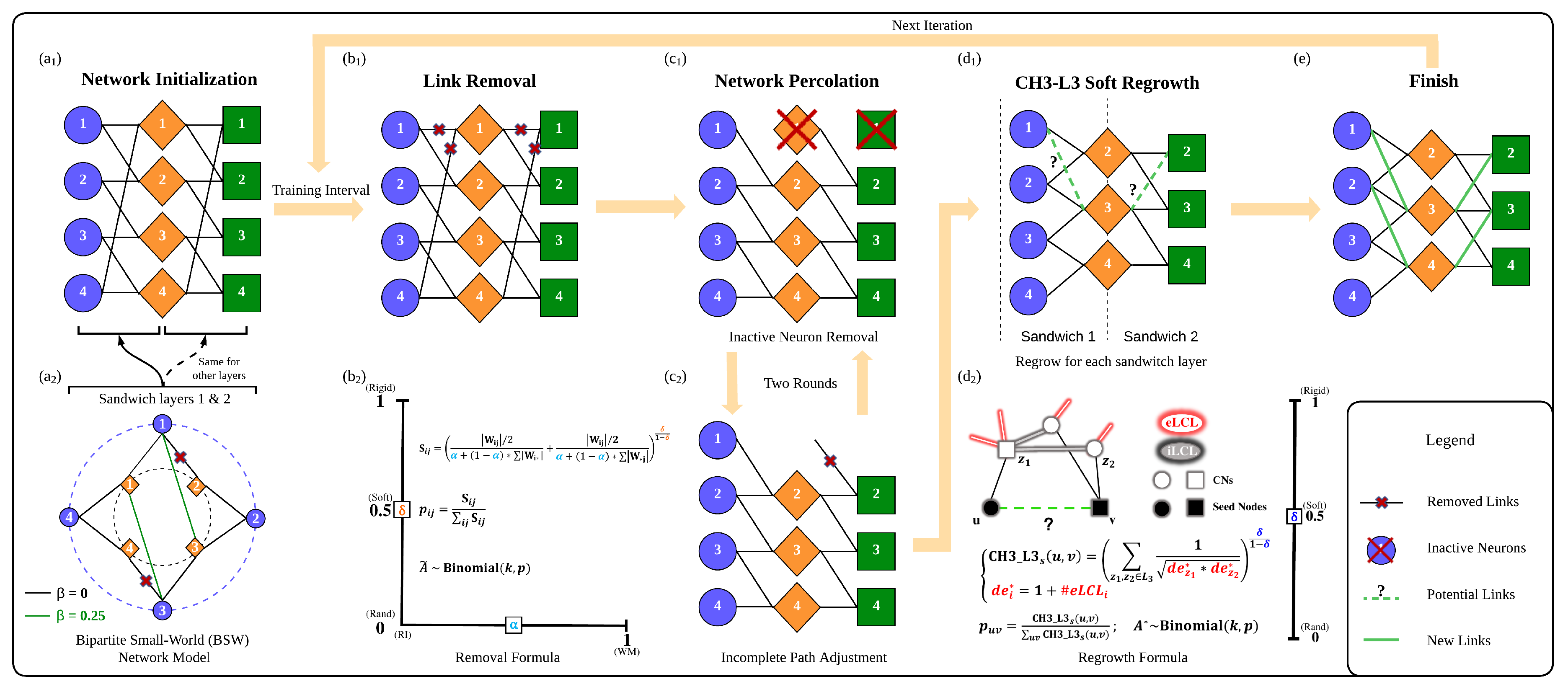
Figure 1. Illustration of the CHTs process. One training iteration follows the path of (a1) -> (b1) -> (c1) -> (c2) -> (d1) -> (e). (a1) Network initialization with each of the sandwich layers being a bipartite small-world (BSW) network. (a2) One sample BSW network with different β values (for β = 0, the network contains the black links; for β = 0.25, the network is formed by removing the marked black links and regrowing the green links). (b1) Link removal process. (b2) Formula for determining which links to remove. (c1) Removal of inactive neurons caused by link removal. (c2) Adjust and remove incomplete links caused by inactive neuron removal. (d1) Regrowth of links according to the CH3-L3-soft rule. (d2) Detailed illustration of the CH3-L3-soft rule. (e) Finished state of the network after one iteration. The next iteration repeats the steps (b1) - (e) from this finished state. A ˜ indicates the removal set of the iteration and A * is the regrown set.
Preprints 109312 g001
Figure 2. The adjacency matrices of the Bipartite Scale-Free (BSF) network model and the Bipartite Small-World (BSW) network model vary with different values of β . a) The BSF model inherently forms a scale-free network characterized by a power-law distribution with γ = 2.76 . b) As β changes from 0 to 1, the network exhibits reduced clustering. It is important to note that when β = 0 , the BSW model does not qualify as a small-world network.
Preprints 109312 g002
Figure 3. The ablation test of each component introduced by CHTs. a) discusses various strategies to improve the Bipartite Scale-Free network model (BSF). EP stands for equal partition of the first layer, and Resort refers to reordering the neurons based on their degree. b) evaluates the influence of the rewiring rate β on the model performance when initialized with the Bipartite Small-World network model (BSW). c) and d) assess the influence of link removal and link regrowth, respectively. We utilize the win rate of the compared factors under the same setting across each realization of 3 seeds for all experiment combinations. The factor with the highest win rate is highlighted in orange.
Preprints 109312 g003
Figure 4. Final performance of CHTs in 99% and 99.9% sparsity on MLP tasks. (a) displays the accuracy of dynamic sparse training (DST) methods alongside their fully connected counterparts (FC) at 99% and 99.9% sparsity levels. The best performances at each sparsity level are highlighted in bold, with performances marked with an asterisk (*) indicating those that surpass FC. (b) shows the active neuron post-percolation rate for the same configurations as in (a), the lowest percolation rates at each sparsity level are highlighted in bold. (c) and (d) present the area across the epochs (AAE) and the ultra-sparse advantage in accuracy plots of 99% sparsity, respectively. The origin point is FC. Scatter points located in the first quadrant indicate models that learn faster and are more accurate than FC. (c) assesses the comparison between Correlated Sparse Topological Initialization (CSTI), the Bipartite Scale-Free (BSF) model and the Bipartite Small-World (BSW) model, selected as the best from Figure 3. (d) assesses the comparison among prevalent dynamic sparse training methods.
Preprints 109312 g004
Figure 5. Percentage change in Accuracy-AAE of CHTs, CHT, RigL, SET with 99% sparsity compared to fully connected counterparts. In every task, CHTs (red) surpasses its fully connected counterparts in both performance and training speed. This indicates that it has gained an ultra-sparse advantage.
Preprints 109312 g005
Table 1. Machine translation BLEU of Transformer trained with CHTs, RigL, SET, and Fully Connected counterparts. All the DST methods are trained with 90% sparsity. The best performance among DST methods is highlighted in bold.
Multi30k IWSLT14 WMT17
FC 31.51 24.11 25.20
CHTs 29.97 21.98 22.43
RigL 28.52 20.73 21.20
SET 28.98 20.09 20.66
Disclaimer/Publisher’s Note: The statements, opinions and data contained in all publications are solely those of the individual author(s) and contributor(s) and not of MDPI and/or the editor(s). MDPI and/or the editor(s) disclaim responsibility for any injury to people or property resulting from any ideas, methods, instructions or products referred to in the content.
Copyright: This open access article is published under a Creative Commons CC BY 4.0 license, which permit the free download, distribution, and reuse, provided that the author and preprint are cited in any reuse.
Prerpints.org logo

Preprints.org is a free preprint server supported by MDPI in Basel, Switzerland.

Subscribe

© 2024 MDPI (Basel, Switzerland) unless otherwise stated