Preprint
Article

On the Complex-Valued Convolutional Neural Network for Oil Spill Classification based on Polarimetric Synthetic Aperture Radar

Altmetrics

Downloads

108

Views

37

Comments

0

Submitted:

17 June 2024

Posted:

17 June 2024

You are already at the latest version

Alerts
Abstract
Marine oil spills seriously threaten the coastal environment, challenge the safety of marine eco-system, and cause huge economic losses to marine fishery, aquaculture, and tourism industries. Timely and accurate oil spill monitoring and early warning can not only make the oil spill acci-dent be handled timely and effectively but also provide key information for investigating the re-sponsibility of the polluters. Polarimetric synthetic aperture radar (SAR) has shown its great po-tential in oil spill classification for its capacity to distinguish mineral oil and biogenic look-alikes. Traditional oil spill classification approaches rely on the scattering matrix elements or pre-designed scattering mechanism-based polarimetric SAR features, which limits its robustness and generalization in large-scale marine surveillance tasks. The recent development of deep learning frameworks, especially the convolutional neural network (CNN) provides a powerful tool for remote sensing image classification. However, conventional CNN only accepts re-al-valued input, which cannot efficiently analyze the polarimetric information carried by com-plex-valued SAR data. In this study, a new framework that employs the complex-valued neural network was proposed for marine oil spill detection. Sophisticated studies were designed to evaluate the contribution of the physical scattering mechanism-based features, complex-valued framework, and convolutional feature extraction structures respectively. Comparative studies were conducted on four study cases using Radarsat-2 and SIR-C fully polarimetric SAR data. The outcome of the proposed study may shed light on the development of an end-to-end marine spill classification system and enlarge its application in practical marine surveillance operations.
Keywords: 
Subject: Environmental and Earth Sciences  -   Remote Sensing

1. Introduction

The Marine oil spill mainly origins from natural hydrocarbon leakage of submarine oil and gas reservoirs, industrial wastewater and domestic sewage discharge, exploitation of offshore oil resources, accidents of ships, drilling platforms, and oil pipelines, illegal discharge by tanker, etc. [1] It has become one of the most common and catastrophic marine accidents. Mineral oil contains a lot of toxic compounds and heavy metals. Once merged into the marine environment, it will seriously threaten the life of marine animals and have a huge impact on aquaculture, salt production, offshore power generation, and seawater desalination industries, and eventually affect people’s health through the food chain.
Remote sensing plays a key role in the early warning, response, and damage assessment of marine oil spills. Compared with optical sensors, SAR has the distinct advantage of all-weather and all-night observation capability, especially under severe weather conditions when oil spill accidents frequently occur. Marine oil spills are usually observed as dark spots on the sea surface due to their suppression of sea surface short and capillary waves [2]. However, many other natural phenomena, such as biogenic oil films, internal waves, low wind speed zones, etc., also form similar bands or patchy dark areas, leading to false alarms, and these can be referred to as oil spill look-alikes. Therefore, distinguishing oil slicks and their look-alikes has become a key issue in SAR marine oil spill observations.
In the early stage, the study of SAR oil spill observation mainly relied on single-polarimetric SAR images. The oil film and look-alikes are classified based on their gray level, texture, and shape information. Therefore, these methods are usually composed of three steps: dark spot detection, feature extraction, and classification [3]. However, oil spill identification with single-polarimetric SAR data usually requires prior knowledge of the oil film and auxiliary information such as sea surface wind speed. However, the state of oil spills on the sea surface is continuously influenced by the complex sea state. For instance, the shape of the oil film on the sea surface is related to the oil type and movement of the oil source during leakage. Therefore, oil spill observation based on single-polarimetric SAR data is difficult to guarantee high accuracy in many cases.
In recent years, oil spill detection based on polarimetric SAR data has become a hot research topic. Polarimetric SAR can obtain detailed backscattering properties of the target and provide more sufficient information for oil spill identification.
Polarization decomposition parameters were first considered for marine oil spill observation. Migliaccio et al. [4] confirmed the effectiveness of these polarimetric decomposition features in sea surface oil film detection based on SIR-C SAR data and proposed a polarimetric CFAR filter for sea surface oil film detection [5]. Nunziata et al. [6] first reported that the polarization pedestal height can reflect the degree of depolarization of ground objects. The pedestal height of open water is lower than that of the oil-covered region, which can be used to effectively distinguish marine oil and its look-alikes.
A series of polarimetric SAR features were proposed based on analyzing the physical mechanism of sea surface backscatter. Nunziata et al. [7] first discovered that the variance of co-polarized phase difference (CPD) can be used as a powerful feature for distinguishing marine oil film and biogenic film. Skrunes et al. [8] analyzed C-band Radarsat-2 and X-band TerraSAR-X data acquired in the North Sea oil spill experiment and compared features including H and α, CPD standard deviation, modulus of HH and VV channel, correlation coefficient and other features on their capability in distinguishing between marine oil and biogenic oil films. Wang et al. [9] used H, α, A, co-polarized correlation coefficient and constitute a new oil spill detection feature for marine oil spill detection.
Although these polarimetric SAR features have proved their effectiveness in some cases, there is still a large gap between their theoretical descriptions and the actual operational situations. Polarimetric features in SAR mages may vary for different cases according to the types, amount, and status of the oil spill. Environmental conditions such as sea surface winds and currents may also have a large impact on the oil spill classification results. Moreover, the configuration of the SAR sensor including polarization modes, incidence angles, resolutions, and calibration issues are also non-neglectable factors. All these problems limit the robustness and generalization of polarimetric features-based approaches in practical marine surveillance tasks.
Conventional machine learning algorithms have limited performance in analyzing large-scale semantic information in SAR images. Deep neural networks have proven their huge advantage in solving complex image classification tasks for their strong non-linear fitting and multi-scale feature extraction capabilities. Among them, Convolutional Neural Networks (CNN) received much research interest for its advantage of properly synthesizing the intensity, texture, and context information. Laurentiis et al. [10] exploited the capabilities of a deep learning framework for learning nonlinear features, shapes, and textural and statistical patterns, in order to obtain significant classification accuracy. Song et al. [11] proposed a novel oil spill identification method based on multi-layer deep feature extraction by CNN. Zhang et al. [12] proposed a deep learning-based oil spill detection framework for quad-polarimetric SAR by using the superpixel model.
However, conventional convolutional neural networks only accept real-valued input. Therefore, the real and complex parts or the intensity and phase information of the polarimetric SAR data must be separately processed. In this way, the integrity of the polarimetric information may be lost and cannot be properly utilized. As a result, how to directly analyze the polarimetric information becomes an urgent research topic. Trabelsi et al. presented a complex-valued convolutional neural network (CVCNN) that takes complex-valued data as its input [13]. Zhang et al. applied CVCNN to the classification of ground objects in polarimetric SAR (PolSAR) images and achieved good results [14]. A previous study has preliminarily demonstrated the potential of CVCNN for marine oil spill classification [15], but more sophisticated analysis remains to be conducted. Moreover, deep learning-based methods have the inherent capability of extracting highly representative features from the original data matrix, therefore, the remained necessity of manually extracting scattering mechanism-based features should be proved.
The key scientific goals for this paper are summarized as follows:
  • To systematically explore the capacities of complex-valued convolutional neural network framework for marine oil spill classification;
  • To quantitatively evaluate the contribution of extracting intensity (semantic) information with convolutional structures in marine oil spill classification;
  • To better understand the role of physical (scattering mechanism) based features extracted from the polarimetric SAR data in various oil spill detection algorithms.
To achieve the above aims, a complex-valued convolutional neural network framework was proposed. Experiments were comprehensively conducted on Radarsat-2 and SIR-C SAR images to evaluate the contribution of each feature processing technique to marine oil spill classification.

2. Methodology

2.1. Polarimetric SAR Features

The fully (or quad-) polarimetric SAR system transmits and receives radar signals under horizontal and vertical polarization bases. In this study, the coherence matrix T derived from fully polarimetric SAR data is considered:
T = T 11 T 12 T 13 T 21 T 22 T 23 T 31 T 32 T 33
Assuming reflection symmetry, T i j equals to T j i . The coherence matrix T contains three real-valued elements (diagonal elements) T 11 , T 22 , T 33 and three complexed valued elements (off-diagonal elements) T 12 , T 13 , T 23 . In this paper, the upper triangular elements of the coherence matrix T are analyzed.
To better describe the scattering mechanism of the sea surface, many features with specific physical significance have been proposed for SAR marine oil spill detection. In this study, the following commonly used features are considered.
(a) Intensity of co-polarized channel
The intensity of the co-polarized channel is a common feature for oil spill detection by single-polarimetric SAR systems. In previous studies, it is believed that generally the signal-to-noise ratio of S V V 2 on the sea surface is higher than that of S H H 2 . Oil spill-covered area has very low radar backscatter due to the damping of surface waves, therefore the intensity of the co-polarized channel is suppressed. However, it is usually challenged by its limitation in distinguishing biogenic look-likes and other physical phenomena that may also result in low backscatter.
(b) H/α Decomposition Parameters
H/α is derived based on the eigenvalue decomposition of the coherency matrix of the target [16]. The three eigenvalues of the coherency matrix T are arranged as λ 1 > λ 2 > λ 3 , U3 is the unitary matrix, whose column vectors, u 1 r , u 2 r and u 3 r are the eigenvectors of T.
T = U 3 λ 1 λ 2 λ 3 U 3 H
Then the probabilities can be calculated from the three eigenvalues:
P i = λ i λ j
Hence, the polarization entropy can be derived by:
H = P i log 3 P i
The mean polarization scattering angle α is defined by:
α = P 1 α 1 + P 2 α 2 + P 3 α 3
The entropy H is a measure of the randomness of the polarization scatter mechanism within the resolution cell. It is base-invariant and closely related to the eigenvalue λ of the coherence matrix, which represents different components of the total scatter power. For a clean sea surface, Bragg scattering dominates, so H is close to 0. While for oil slick-covered areas, the scattering mechanism gets much more complex, and the stronger random scattering results in higher entropy. However, for biogenic slicks, although the scattering power is lower, the main scattering mechanism is still Bragg [17], resulting in low entropy similar to a clean sea surface. Therefore, H can be used to distinguish oil slicks and weak damping look-alikes. [17] The mean scattering angle α represents the main scattering mechanism of the target. On slick-free marine surfaces, α is usually less than 45° as the Bragg scattering is dominant. In slick-covered regions, a more complex scattering mechanism is present and much larger α can be measured.
(c) Ellipticity χ
Ellipticity χ describes the polarimetric ellipse’s shape of the scattered EM wave:
sin 2 χ = S 3 m S 0
where S3 is the element of Stokes vector and m stands for the degree of polarization of the received EM wave. χ can be employed as an indicator of the scattering mechanism. For slick-free sea surfaces where Bragg scattering is dominant, the sign of χ is negative. For oil-covered sea surfaces, as a more random scattering mechanism is present, χ will be larger and can become positive [18]. This feature makes χ a logical binary descriptor of slick-free vs. oil-covered areas.
(d) Pedestal Height
In the co-polarized signature of the scene, the normalized radar cross-section (NRCS) σ0 is a function of both the tilting angle Φ and the ellipticity χ of the polarization ellipse. The pedestal height (PH) is defined as the lowest value σ0 in the co-polarized signature when the tilting angle Φ and the ellipticity χ change. The PH describes the unpolarized energy of the total scattering power and behaves as a pedestal on which the co-polarized signature is set [19]. The normalized pedestal height (NPH) can be defined as the minimum eigenvalue divided by the maximum eigenvalue:
N P H = min λ 1 , λ 2 , λ 3 max λ 1 , λ 2 , λ 3
For a clean sea surface, the scattering mechanism is pure Bragg, so an NPH value close to 0 is expected. While for the oil-covered area, much higher NPH can be expected due to the non-Bragg scattering that reflects a more diverted scattering mechanism.
(e) Co-Polarized Phase Difference
The co-polarized phase difference (CPD) is defined as the phase difference between the HH and VV channels [7]:
φ c = φ H H φ v v
From multi-looked SAR data, it can be also derived as:
φ c = arg < S H H S V V >
where arg(*) stands for phase calculation.
The standard deviation of CPD is a very efficient parameter indicating sea surface scattering mechanisms [7]. It can be counted from φ c using a sliding window. On slick-free sea surfaces, the correlation between HH and VV channels is high, and a narrow CPD distribution is expected. This results CPD in having a small standard deviation, and it is the same for weak-damping (biogenic slicks)-covered areas. In marine oil slicks-covered regions, the Bragg scattering is weakened while other scattering mechanisms increase, and the HH-VV correlation largely decreases. As a result, the pdf of CPD becomes broader, and its standard deviation largely increases.
(f) Conformity Coefficient
The conformity coefficient was first used in compact polarimetric SAR applications for soil moisture estimations [20]. In a full polarization scheme, its proxy is defined as [21]:
μ = 2 R e S H H S V V S H V 2 S H H 2 + 2 S H V 2 + S V V 2
The conformity coefficient μ evaluates whether surface scattering is dominant among all the scattering mechanisms. For a slick-free sea surface, Bragg scattering results in a very small cross-polarized backscattering power and results in high HH-VV correlation: R e S H H S V V > S H V 2 ; hence, μ is positive. However, for hydrocarbon(biogenic oil)-covered areas, as non-Bragg scattering exists, HH-VV correlation is lower, and cross-pol component largely increases, which is very likely to have: R e S H H S V V < S H V 2 , resulting in negative μ. For weak-damping cases such as biogenic slicks, since Bragg scattering is still dominant, R e S H H S V V > S H V 2 is still valid and results in positive μ. Under this rationale, conformity coefficients can be used to effectively distinguish hydrocarbon slicks from biogenic slicks.
(g) Correlation and Coherence Coefficients
The correlation and coherence coefficients are derived from the coherence matrix by [8]:
ρ H H V V = a b s < S H H S V V > < S H H 2 > < S V V 2 >
C o h = < T 12 > < T 11 > < T 22 > )
where T i j is an element of the coherence matrix T.
These two parameters both range between 0 and 1. For a slick-free area, HH and VV channels are highly correlated, so they are expected to be very close to 1. For an oil-covered sea surface, a much lower HH/VV correlation is expected, so the correlation and coherence coefficients are both much lower.

2.2. Principles of Neural Networks

2.2.1. Real-Valued Neural Networks

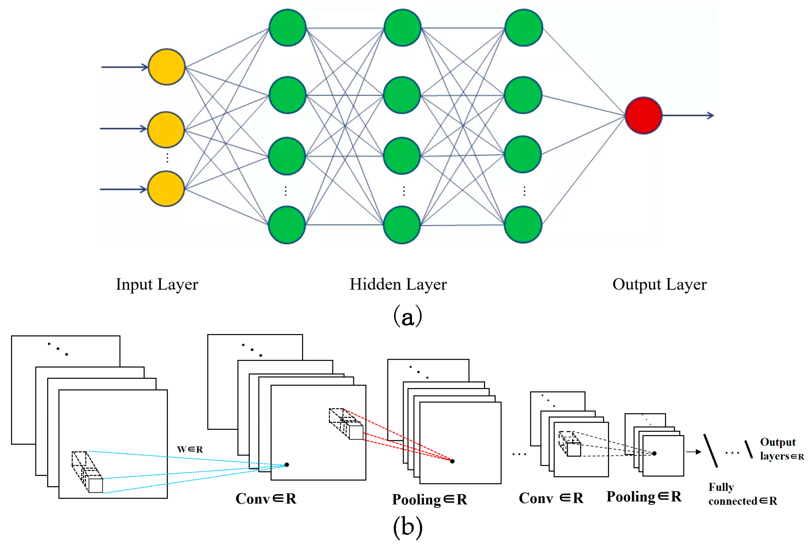
In this paper, two types of real-valued neural networks were considered, including real-valued artificial neural network (RVANN), and real-valued convolutional neural network (RVCNN). RVANN is a nonlinear system composed of many interconnected processing units and has the characteristics of self-adaptation, self-organization, and real-time learning. A demonstration of the structure of an RVCNN is shown in Figure 1a, which includes the input layer, hidden layers, and output layer. In the fields of image classification and target detection, the convolutional neural network has shown superior performance. RVCNN extracts rich features by using a convolutional layer, alternates the feature dimensions by pooling layer, and finally outputs classification results through a fully connected layer. RVCNN shares parameters between layers, to obtain location consistency analysis capability. The typical structure of an RVCNN is shown in Figure 1b, which includes an input layer, convolutional layers, pooling layers, a fully connected layer, and an output layer.

2.2.1. Complex-Valued Neural Networks

In this work, the CVCNN framework in [13,14] is properly adjusted for marine oil spill detection tasks.
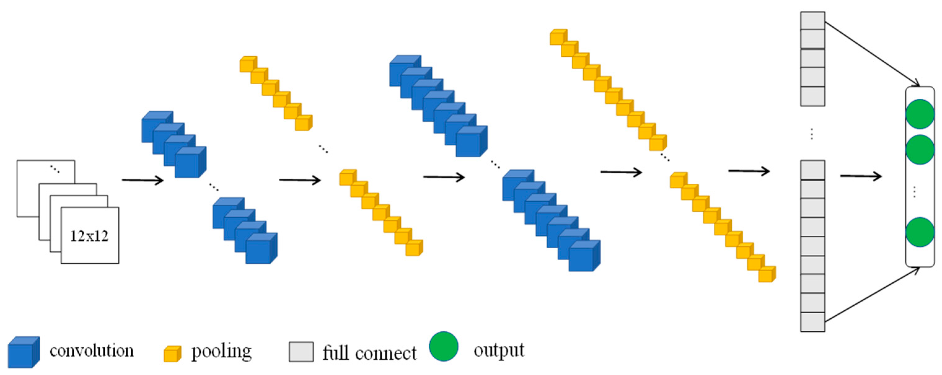
Different from the RVCNN, the weights, and bias of CVCNN, for all the input and output layers, are defined in the complex domain. The network structure of a typical CVCNN is shown in Figure 2.
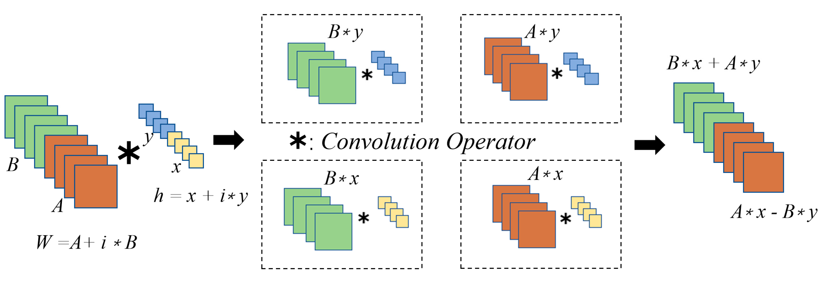
The inputs of a CVCNN are complex numbers, of which the real part A and imaginary part B are expressed as different real numbers. In the convolutional layer, complex convolution operations can be expressed as:
W h = A x B y + i B x + A y
Or in the form of the matrix:
R e W h I m W h = A B B A x y
where h is the network input, which is a complex vector h = x + i*y; W is the weight, which is a complex matrix W =A+ i*B. R e   is the real part of the complex number, and I m   stands for its imaginary part. A more intuitive representation of the complex convolutional operation process is shown in Figure 3.
When cascaded, the output of the (l+1)th convolution layer is obtained by passing a nonlinear activation function:
O i l + 1 = f R e I i l + 1 + i × f I m I i l + 1
where:
I i l + 1 = k = 1 K O k l w i k l + 1 + b i l + 1 = k = 1 K R e O k l × R e w i k l + 1 I m O k l × I m w i k l + 1 + i k = 1 K I m O k l × R e w i k l + 1 + R e O k l × I m w i k l + 1 + b i l + 1
where, O i l + 1 represents the value of the output feature map of the convolutional layer after activation function, I i l + 1 represents the output feature map of the convolutional layer, O k l represents the input feature map of the current convolutional layer, and w i k l + 1 represents the weight matrix, that is, the convolution kernel. b i l + 1 represents the bias.
Accordingly, the ComplexReLU (CReLU) function is used as the complex activation function in CVCNN:
C R e L U ( z ) = R e L U ( R e ( z ) + i R e L U ( I m ( z ) )
where, R e   eans the real part of the complex number, and I m   means its imaginary part.
Just as traditional RVCNN, CVCNN continuously optimizes the weights and biases through supervised training, so that the network output matches the given label of the training data, making the difference between them smaller and smaller. The error between the output classification result and the target can be described as the loss function E l o s e , which is expressed using the classical least square error MSE. Set the input value to { I k , L k }, I k denotes the kth input sample, O k represents the predicted value of the kth input sample, L k is the label of the sample, then:
E l o s e = 1 2 N k = 1 K R e O k R e L k 2 I m O k I m L k 2
The weight and bias are initialized through random initialization and updated with stochastic gradient descent (SGD). In the training process, the updating rules of the weight and bias are as follows:
w i k l + 1 t + 1 = w i k l + 1 t + Δ w i k l + 1 t = w i k l + 1 t η E l o s e t w i k l + 1 t
b i l + 1 t + 1 = b i l + 1 t + Δ b i l + 1 t = b i l + 1 t η E l o s e t b i l + 1 t
Where η stands for the learning rate, and the complex backpropagation of weight is conducted by:
E lose   w i k I + 1 = E lose   Re w i k l + 1 + E lose   I m w i k l + 1 = E lose   R e I i l + 1 R e I i l + 1 R e w i k l + 1 + E lose   I m I i l + 1 Im I i l + 1 Re w i k l + 1 + i E lose   Re I i l + 1 R e I i l + 1 I m w i k l + 1 + E lose   I m I i l + 1 I m I i l + 1 I m w i k l + 1
Similarly, the update of the bias quantity b i l + 1 can be conducted.
Moreover, to fully verify the contribution of complex information to oil spill classification, we expand the RVANN to the complex domain similarly and formalize a complex-valued artificial neural network (CVANN) for a fair comparison.

2.3. Evaluation Indexes

The confusion matrix depicts the number of correct classifications of each feature and the number of misclassified categories and numbers, the overall accuracy (OA) refers to the ratio of the number of correctly classified pixels to the total number of pixels. The Kappa coefficient is an index used to measure whether the prediction results of the model are consistent with the actual classification results.
K a p p a = X n n i = 1 n 1 X i i i = 1 n 1 X i n X n i X n n 2 i = 1 n 1 X i n X n i
O A = i = 1 n 1 X i i X n n
The F1 score is used in statistics to measure the accuracy of a binary classification model. It takes into account both the precision and recall of the classification model. The F1 score can be regarded as a harmonic average of the model's precision and recall, with a maximum value of 1 and a minimum value of 0. The receiver operating curve (ROC) combines sensitivity and specificity with a graphical method, which can accurately reflect the relationship between specificity and sensitivity of an analytical method and is a comprehensive representative of test accuracy.

2.4. Procedure of the Experiments

The procedure of the whole study is presented in Figure 4.
Firstly, the original Radarsat-2 and SIR-C SAR data were preprocessed, including ROI cropping and Refined Lee filtering, to concentrate on the target and obtain images with lower speckle noise.
Secondly, nine classical polarization features were extracted from the pre-processed SAR data, and a feature selection framework was built based on the Pearson correlation coefficient, J-S divergence and ReliefF algorithm to decide the optimal combination of polarization features for marine oil spill classification.
Thirdly, real and complex-valued feature sets were generated. Based on the feature selection results, the combined feature sets were established to evaluate the contribution of these scattering mechanism based polarimetric features.
Fourthly, oil spill classification were conduced. A CVCNN model for oil spill classification is proposed, and the basic procedure of the network model is derived, including parameter initialization, complex-valued convolution, complex-valued pooling, complex-valued full connection, and output. The backpropagation, Batch Normalization layer and activation function are also adjusted to complex-valued data flow. RVANN, RVCNN and CVANN models were also evaluated for comparative study.
The K-fold cross-validation is used to evaluate the performance of the proposed CVCNN and other models in marine oil spill classification based on polarimetric SAR data. The classification maps, overall accuracy and ROC curve were used to evaluate the experimental results to verify the robustness and generalization performance of the model.
3. Experiment and Results

3.1. Dataset

In this paper, experiments were conducted on Radarsat-2 and SIR-C fully polarimetric SAR data obtained in four study cases respectively.
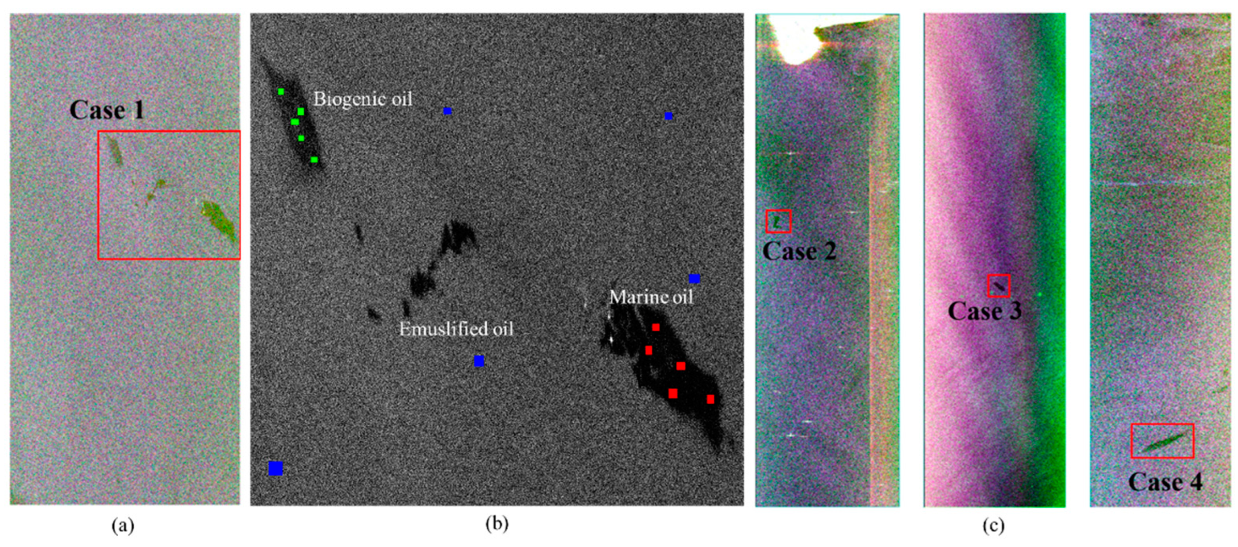
In Case 1, the Radarsat-2 image is acquired from the oil-on-water exercise conducted by the Norwegian Clean Seas Association for Operating Companies (NOFO) in the North Sea (N59°59', E2°27') on 2011-06-09 [22]. During the exercise, different substances were deployed onto the sea surface, including biogenic oil, emulsified oil, and mineral oil. 2-Ethylhexyl oleate, a monoalkyl ester of oleic acid named Radiagreen ebo was used to simulate the monomolecular biogenic film. The evaporated Balder oil was deployed as the mineral oil, and the emulsified oil was formed by Oseberg blend mineral oil mixed with 5% IFO380, with a water content of 69% [23]. Because the emulsified oil film has a status between mineral oil film and biogenic oil film, the classification of emulsified oil film is not considered in this paper. Figure 5a shows the PauliRGB image of the study case, the region bounded by the red box has been selected for the experiment, Figure 5b shows the VV power image of the study region in Case 1, and the manually labeled data samples for this study, in which red represents marine oil, cyan represents biogenic oil, and blue represents clean seawater; Figure 5c are SAR images acquired during the SIR-C mission: Case 2 is obtained on 1st October 1994, 8:14 UTC (processing number: p.n. 44327), in which an oil spill is clearly visible. Case 3 is relevant to the SIR-C acquisition of 15th April 1994, 2:14 UTC (processing number: p.n. 11588), in which an OLA is clearly visible. Case 4 is a typical oil spill pattern due to ship emission acquired by SIR-C on 8th October 1994 (processing number: p.n. 49939). No information about the type of oil is reported in the literature. [25] Refined Lee filtering was performed on the four SAR images respectively to suppress speckle noise.

3.2. Configurations of Feature Sets

As introduced in section 2.1, following the reciprocity rule, all the polarimetric information within coherence matrix T can be represented by its six upper triangular elements. For the complex-valued neural network, a feature vector F T c can be formalized as the input:
F T C = T 11 , T 12 , T 13 , T 22 , T 23 , T 33
For real-valued networks, the real and image parts of the complex-valued element in T are separately input, therefore the corresponding real-valued feature set F T R is:
F T R = T 11 , T 12 _ r e a l , T 12 _ i m a g , T 13 _ r e a l , T 13 _ i m a g , T 22 , T 23 _ r e a l , T 23 _ i m a g , T 33
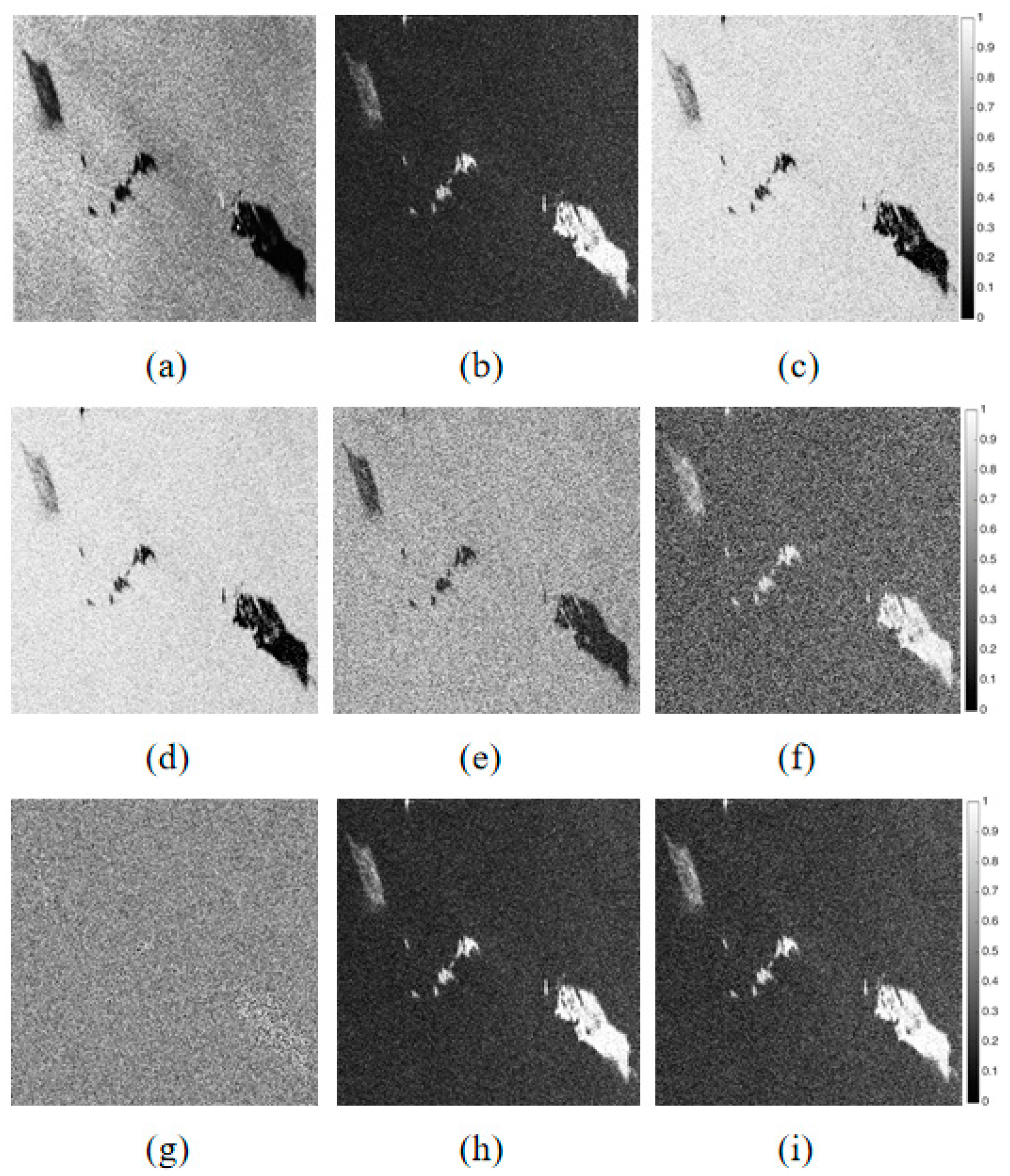
As shown in Figure 6, the 9 polarimetric features introduced in section 2.1 are extracted from the RADARSAT-2. It can be observed that the biogenic slicks (upper left) and mineral oil (lower right) both show very low S V V   2 manifesting the limited capability of intensity-based features in oil spill classification. For the rest polarimetric features (b)-(i), much larger differences between mineral and its biogenic look-alikes can be observed.
Theoretically, inputting high-dimension feature sets to a neural network, the data samples will become relatively insufficient to derive a converged training result. This is because the training samples will become significantly sparser when they are embedded into a higher-dimension feature space. This phenomenon is called the “curse of dimensionality”. Moreover, high input dimension also comes with large memory requirements and an increased computation burden. Therefore, it is necessary to reduce the feature dimension of marine oil spill classification models. In this study, feature selection was conducted by evaluating the importance of polarimetric features to oil spill classification on the sea surface to reduce the feature dimension while maintaining their key polarimetric information.
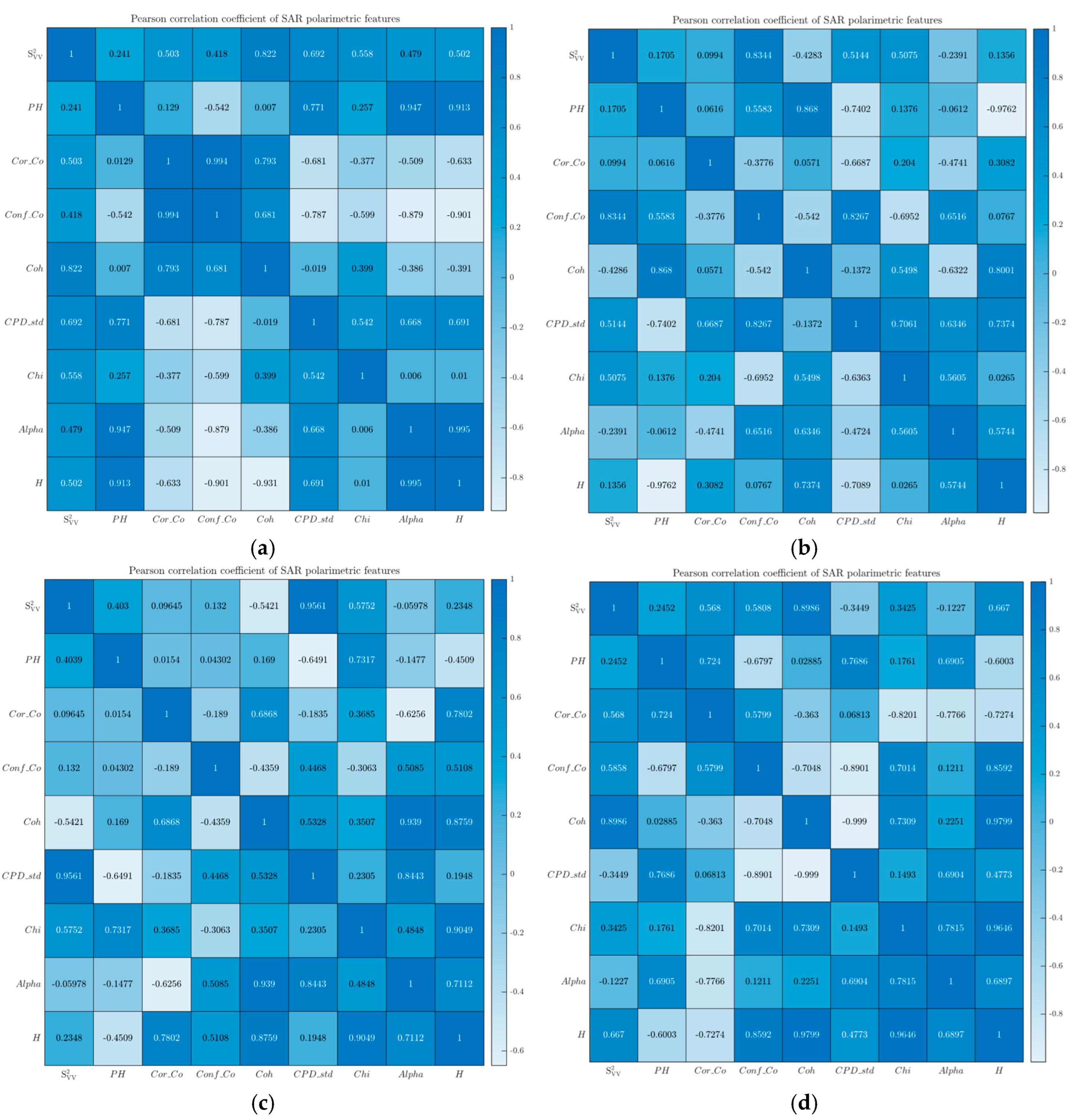
Pearson correlation analyses were conducted on polarimetric features extracted from the four study scenes respectively to evaluate the correlations of these features. A correlation higher than 0.6 or lower than -0.6 indicates a relatively high positive or negative correlation. As shown in Figure 7a, feature pairs between S V V 2 and Coh, S V V 2 and CPD-std, PH and CPD-std, PH and Alpha, PH and H, Cor_Co and Conf_Co, Cor_Co and Coh, Cor_Co and CPD-std, Cor_Co and H, Conf_Co and Coh, Conf_Co and CPD-std, Conf_Co and Alpha, Conf_Co and H, CPD-std and Alpha, CPD-std and H, Alpha and H shows high correlation within the RadarSAT-2 dataset. For the other three scenes acquired by SIR-C, a high correlation between feature pairs can also be observed, among them PH and CPD-std, H and Coh, Alpha and CPD-std, H and PH are relatively consistence ones. High correlation (positive or negative) indicating that these features contain abundant linear relevant information, the dimension of the input polarimetric feature sets should be compressed.
Polarimetric features from three types of targets, namely mineral oil, biogenic film and clean sea water, are analyzed by calculating the J-S divergence between them. A J-S divergence value greater than 0.8 or 0.6 indicates excellent or good separability. Table 1 and Table 2 shows the J-S divergence of the extracted polarimetric features between target pairs of Mineral oil-Biogenic film, Mineral oil-Clean water and Biogenic film-Clean water within the four study cases.
According to the J-S divergence analysis results, the following features have excellent or good capabilities in separating Mineral oil spill, Biogenic film, and Clean sea water: S V V 2 , H ,   C o h ,   C o r _ C o , P H , C o n f _ C o , A l p h a .
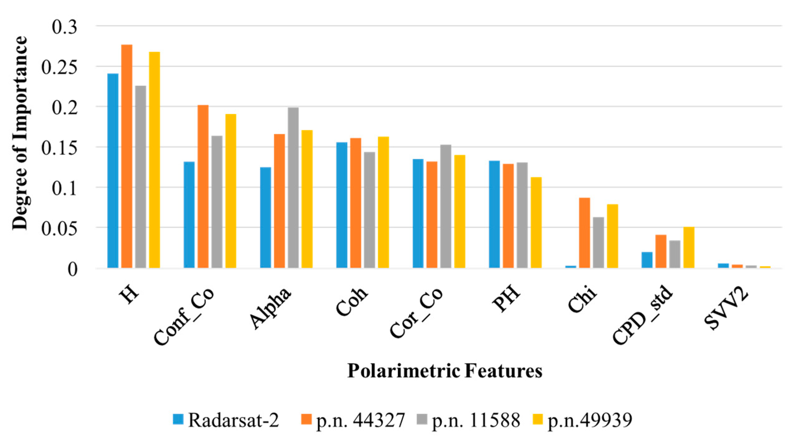
Then the ReliefF algorithm is applied to analyze the importance of each polarimetric feature from the perspective of class separability. When dealing with multi-class problems, the ReliefF algorithm randomly takes a sample R from the training sample set each time, and then finds the k nearest hits (near Hits) of R from the sample set of the same type as R. It finds the k nearest neighbor samples (near Misses) in the sample set, and then update the weight of each feature, representing the importance of which in the classification task [25]. As can be observed in Figure 8, the following six features have a relatively higher importance in oil spill classification: H ,   C o h ,   C o r _ C o , P H , C o n f _ C o , A l p h a .
Comparing the selected feature sets based on J-S divergence and the ReliefF algorithm, they are mostly consistent with each other. The only difference is S V V 2 , which manifests the consistent target classification capabilities of features. The extremely low index of S V V 2 derived by ReliefF may be result from its limited capabilities in distinguishing mineral oil and biogenic look-alikes. Moreover, the backscattering intensity information carried by S V V 2 is also highly correlated with feature T11 in the coherent matrix. Therefore, S V V 2 is excluded from the final polarimetric feature set in the upcoming study:
F P = H ,   C o h ,   C o r _ C o , P H , C o n f _ C o , A l p h a
To evaluate the added contribution of the above scattering mechanism-based polarimetric SAR features to marine oil spills classification, they are combined with real- and complex-valued features directly derived from the coherence matrix T respectively, and formed the following two feature sets:
F T C , F P = T 11 , T 12 , T 13 , T 22 , T 23 , T 33 , H ,   C o h ,   C o r _ C o ,   P H ,   C o n f _ C o ,   A l p h a
F T R , F P = T 11 , T 12 _ r e a l , T 12 _ i m a g , T 13 _ r e a l , T 13 _ i m a g , T 22 , T 23 _ r e a l , T 23 _ i m a g , T 33 , H ,   C o h ,   C o r _ C o ,   P H ,   C o n f _ C o ,   A l p h a
To summarize, totally four feature sets, F T C , F T R , F T C , F P , F T R , F P are considered in the study for revealing the mechanism of classification models from the following two aspects. On one hand, comparing the feature groups F T C , F T R and F T C , F P , F T R , F P aims to explore the advantage of the proposed complex-valued framework; on the other hand, comparing the feature groups F T C , F T C , F P and F T R , F T R , F P intends to explore the role of the scattering mechanism-based polarimetric features in the proposed classification framework. Moreover, within the above evaluation framework, the performance of oil spill classification approaches based on ANN and CNN were compared to evaluate the contribution of analyzing semantic information for oil spill classification.

3.3. Detailed Model Configurations and Sample Selection Method

To avoid the interference induced by the network structure, the layer configurations of the two networks employed in this study are kept as consistent as possible. Figure 9 shows the basic network structure of the proposed CVCNN and RVCNN, which has two convolution layers and one average pooling layer. The network has three types of output, namely marine oil, biogenic film, and seawater. More implementation details of the CNN models used in this experiment are listed in Table 3.
To overcome the interference of sample selection on model training, the experiment adopts a 10-fold cross-validation, with the ratio between the training set and test set as 9: 1. To ensure that the number of samples in the sea surface (sea water) and the oil slick area (oil film) without oil slick is equal. For the Radarsat-2 data, 1800 samples (including 900 oil film samples and 900 seawater samples) were randomly selected as the training set, while 200 samples (including 100 oil film samples and 100 seawater samples) were selected as the test set. For SIR-C data, 900 samples (including 450 oil film samples and 450 seawater samples) were randomly selected for each scene as the training set, and 100 samples (including 50 oil film samples and 50 seawater samples) were selected as the test set. Each sample was assigned as the testing set for once alternatively during the cross-validation, and finally, the evaluation indexes derived from the 10 repetitions were averaged as the evaluation result. Finally, the evaluation indexes derived from the 10 turns are averaged as the result.

3.4. Oil Spill Classification Results

3.4.1. Experiment on Radarsat-2 Data

a)
Study on the real- and complex-valued neural networks for marine oil spill classification
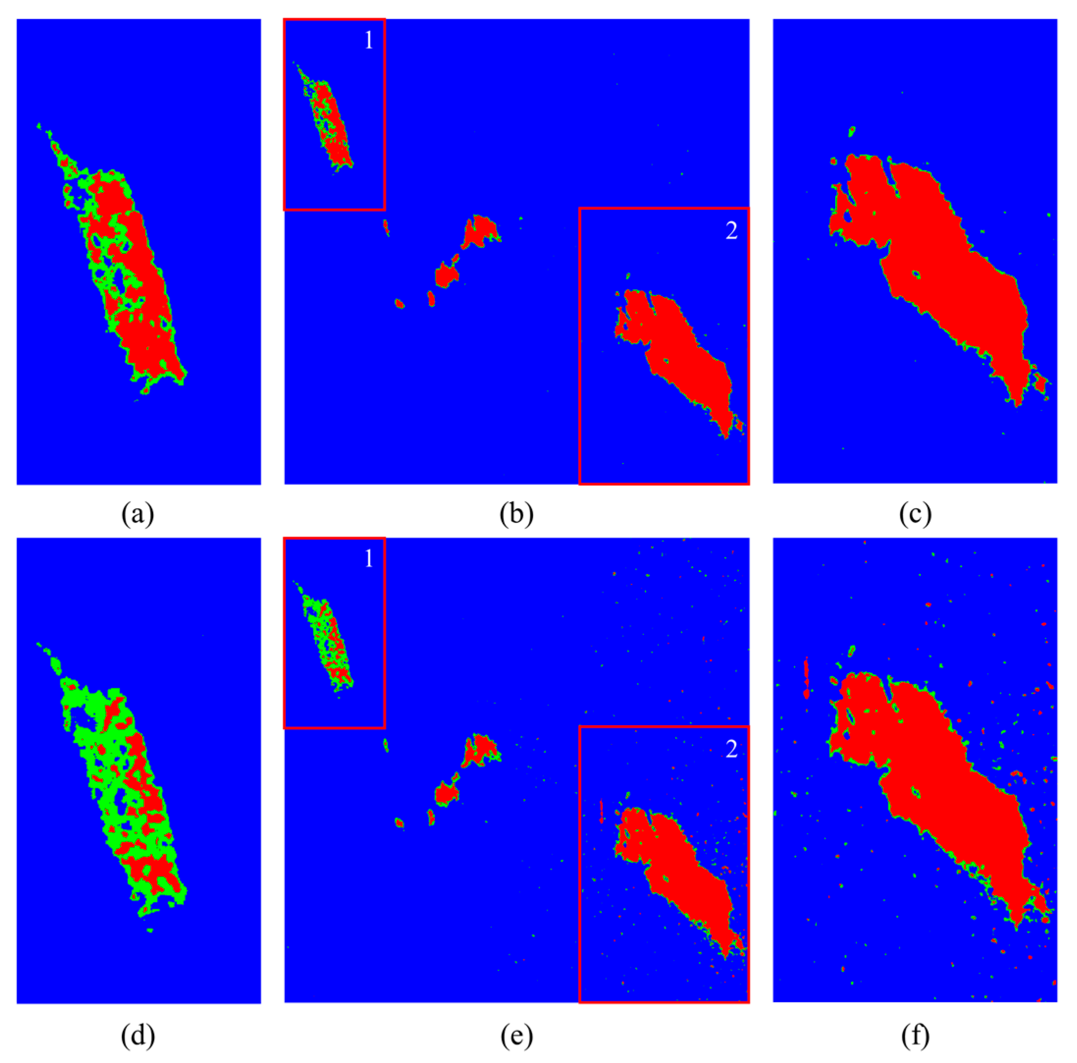
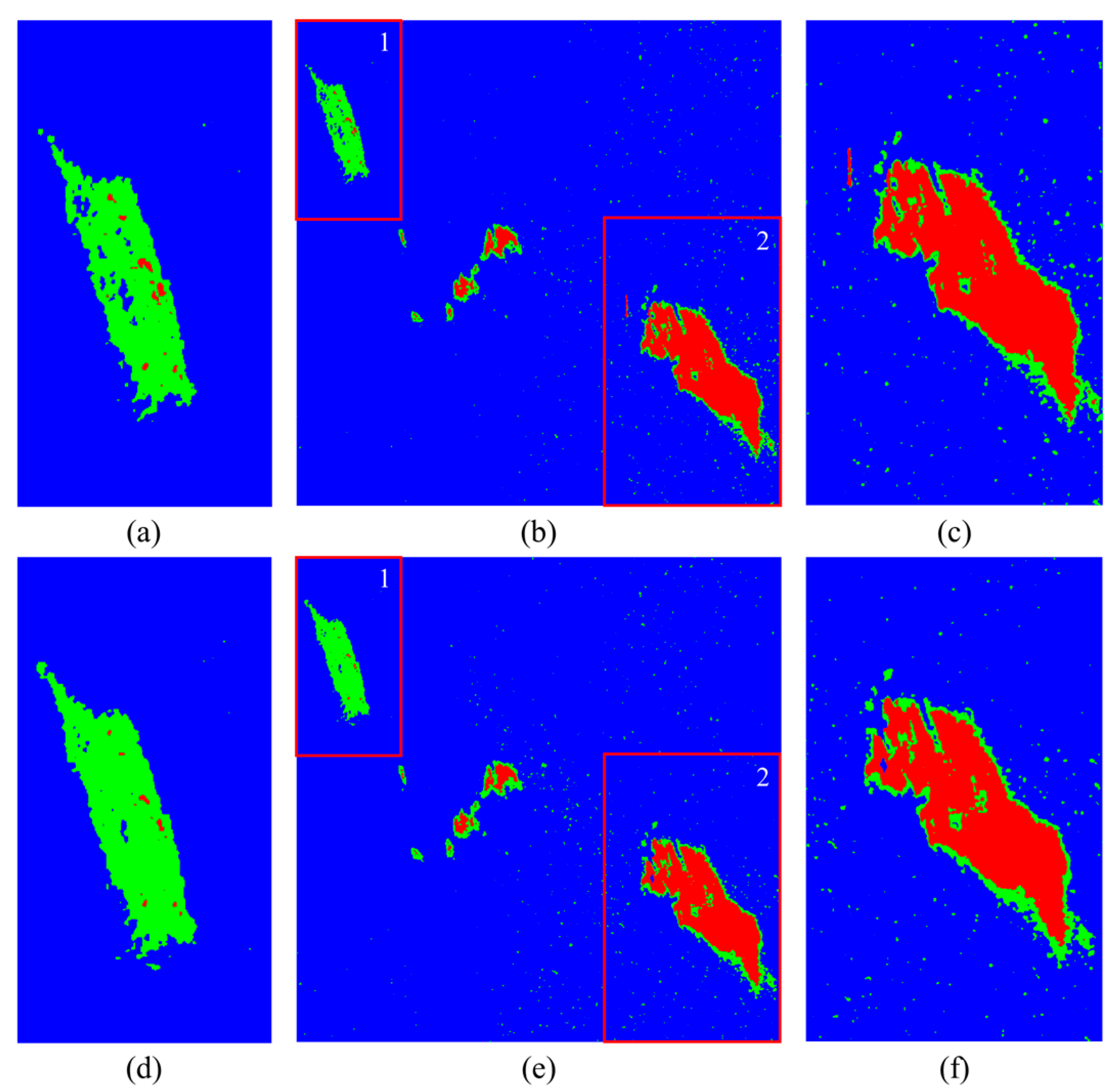
The classification results derived by RVANN and CVANN are shown in Figure 10. It can be observed that the misclassification can be mainly attributed to the following aspects: (1) Some pixels in the seawater area are mistakenly divided into more biogenic oil; (2) Some pixels around mineral oil are misclassified as biological oil; (3) Some pixels in the biogenic oil are misclassified into mineral oil. Comparable results are obtained by CVANN and RVANN models. The main difference is that more pixels around mineral oil and on the clean sea surface are misclassified as biogenic film by CVANN and slightly more pixels within the biogenic slicks are misclassified into mineral oil film by RVANN.
In Figure 11, the classification results derived by RVCNN and CVCNN are presented. Generally, a very similar tendency as in Figure 10 can be observed. The CVCNN model generally outperforms RVCNN mainly by limiting the misclassification on the biogenic film.
As inspected from the classification maps, among the above four compared classification models, CVCNN achieves generally the best overall oil spill classification results.
b)
Study on the role of polarimetric scattering mechanism-related features in oil spill classification
Keeping the similar network structure applied in the previous analysis, polarimetric scattering mechanism-related features are introduced and formed feature sets F T C , F P and F T R , F P as the input respectively.
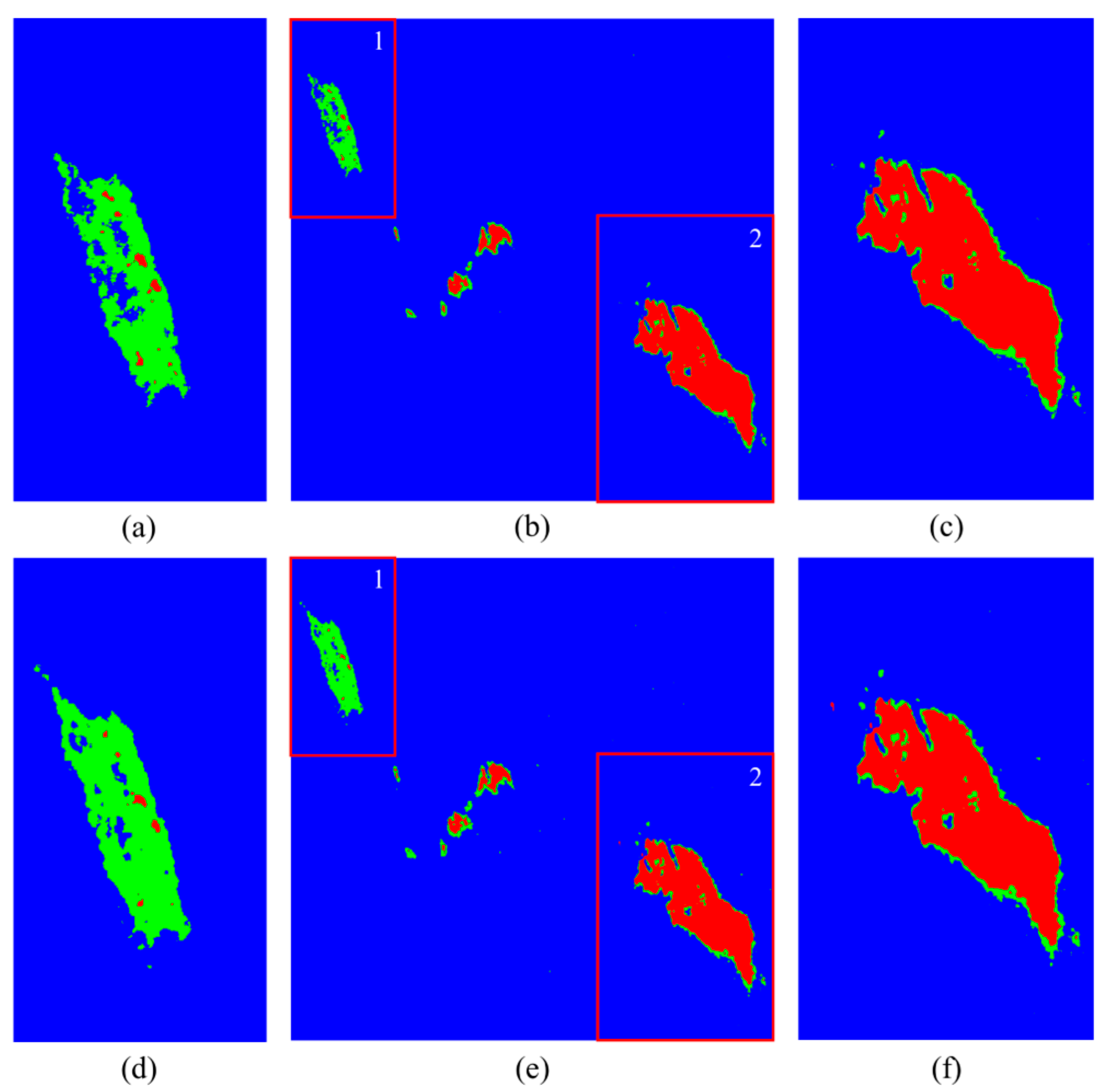
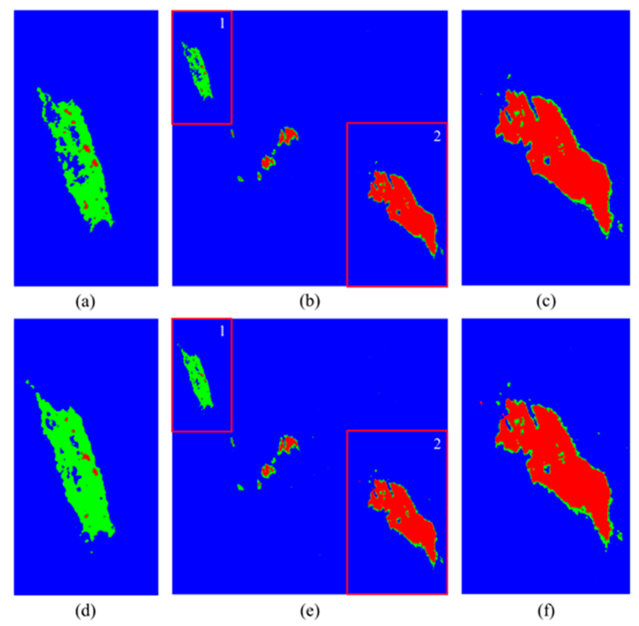
In Figure 12 and Figure 13., it can be found that compared with inputting only elements of T, the four classification models obtained a significant performance improvement. It can be observed that most targets in the study scene are correctly classified, except for the pixels on the edge of mineral oil. Further better results were obtained by RVCNN and CVCNN than CVANN and RVANN, demonstrating the contribution of utilizing spatial information. According to the zoomed in sub-figures, CVCNN has a slightly better performance mainly in controlling the misclassification to biogenic film within the mineral oil region than RVCNN.
The overall accuracy derived on the Radarsat-2 dataset during the above experiments is summarized in Table 6. In accordance with previous visual inspection results, CVCNN reaches the highest accuracy of 94.86% when inputting scattering mechanism-based polarimetric features along with complex-valued features in T. Then followed by the classification results achieved by RVCNN by inputting polarimetric features along with real-valued features in T. Generally, complex-value based models obtained slightly higher OA than real-value based models, and CNN-based models achieved higher performance than ANN-based models. Moreover, when adding scattering mechanism-based features as the input, the derived OA differences between real- and complex-valued models significantly increased.

3.4.2. Further Results on the SIR-C Datasets

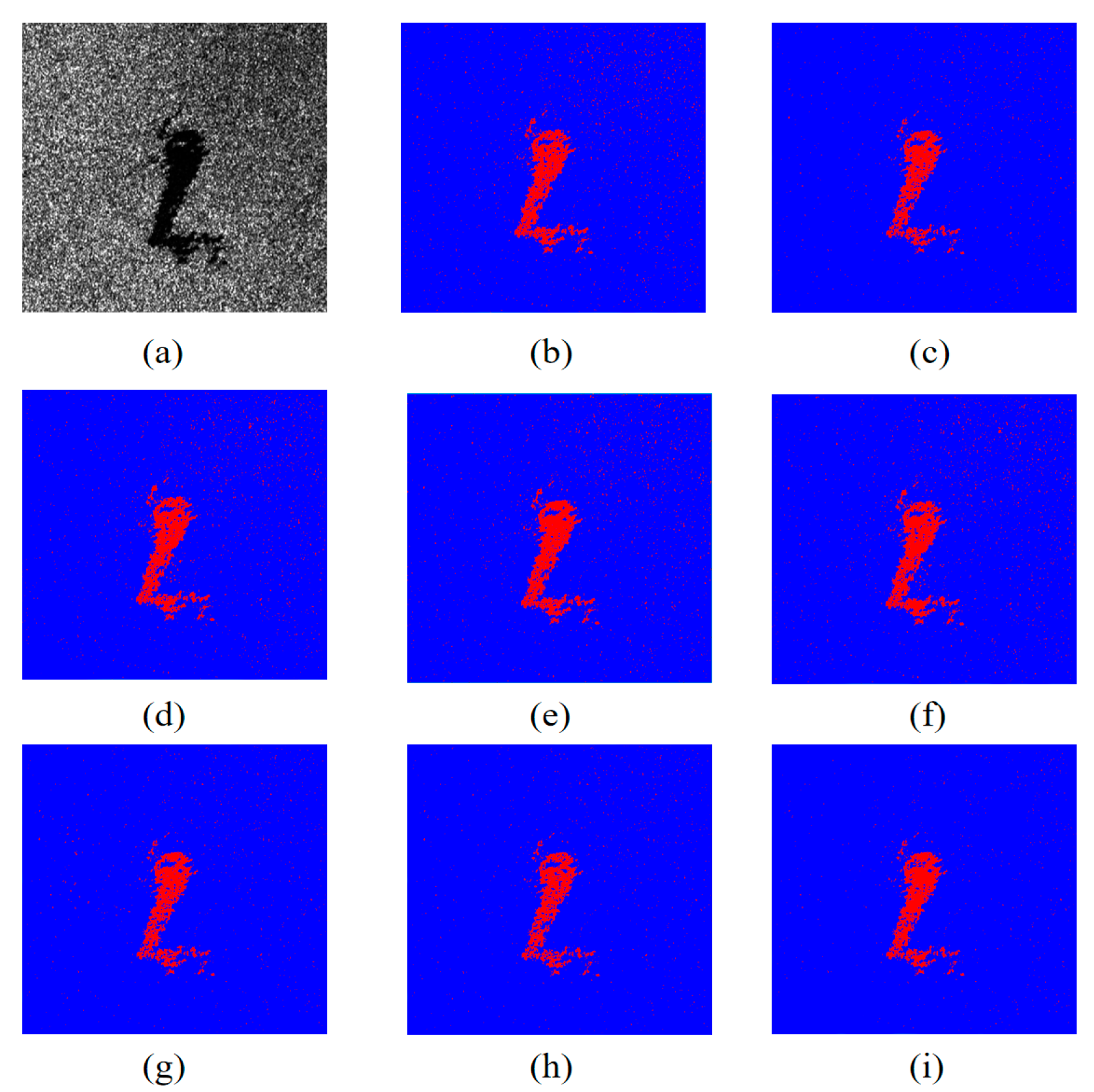
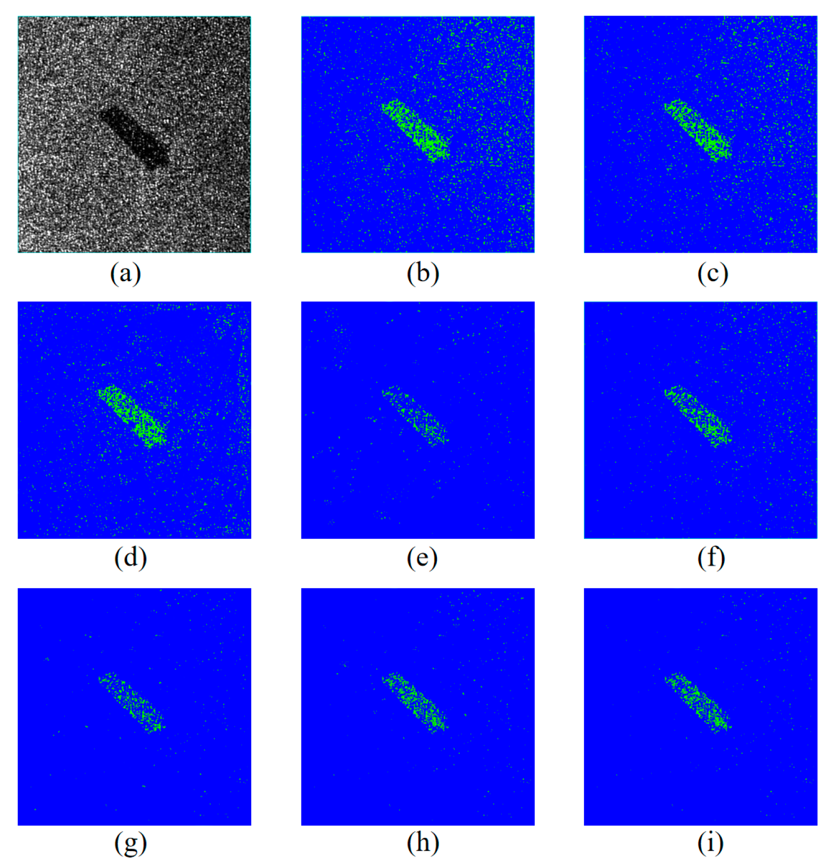
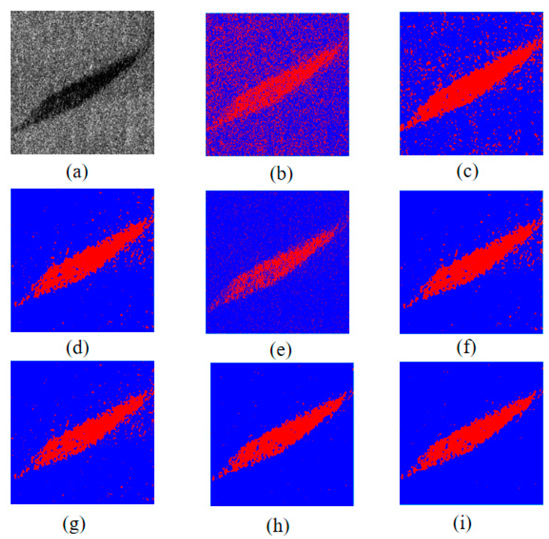
Experiments were conducted on the SIR-C dataset with the scene number p.n. 44327, p.n. 11588, and p.n. 49939 following similar training and testing procedures, to further verify the result of this study. In p.n. 44327 and p.n. 49939, mineral oil films are present, whereas in p.n. 11588, there is a biogenic slick. The classification maps are shown in Figure 14, Figure 15 and Figure 16 respectively, where red represents the identified mineral oil, green represents biogenic film, and blue represents seawater. Table 7, Table 8 and Table 9 shows the OA of each classification model derived by different classifier classifiers and feature inputs.
Although the classification accuracy is different on each dataset, CVCNN model uniformly obtained the best classification map and overall accuracy when taking F T C , F P as the feature input. As expected, the classification accuracy improves after considering complex-valued information, and the introduction of the polarimetric features significantly improves the classification ability of the model. In addition, the convolutional network structure performs better than the fully connected network in this classification task under both real-valued and complex-valued feature input. It should be noted that in this experiment, compared with using the complex-valued framework, introducing the polarimetric features has a larger improvement on the classification ability of the model, except for p.n. 49939.
The classification maps derived from the SIR-C datasets are generally in accordance with the OA results, as shown in Figure 14, Figure 15 and Figure 16. The complex-valued models applied in this study outperform their real-valued competitors, while CNN-based models achieve slightly higher performance for their capability of taking texture and semantic information into consideration. Moreover, the introduction of scattering mechanism-based feature sets significantly improves the classification accuracy of the model, mainly by improving the integrity of the targets and reducing the false alarm on the clean sea surface.

3.4.3. Further Quantitative Analysis

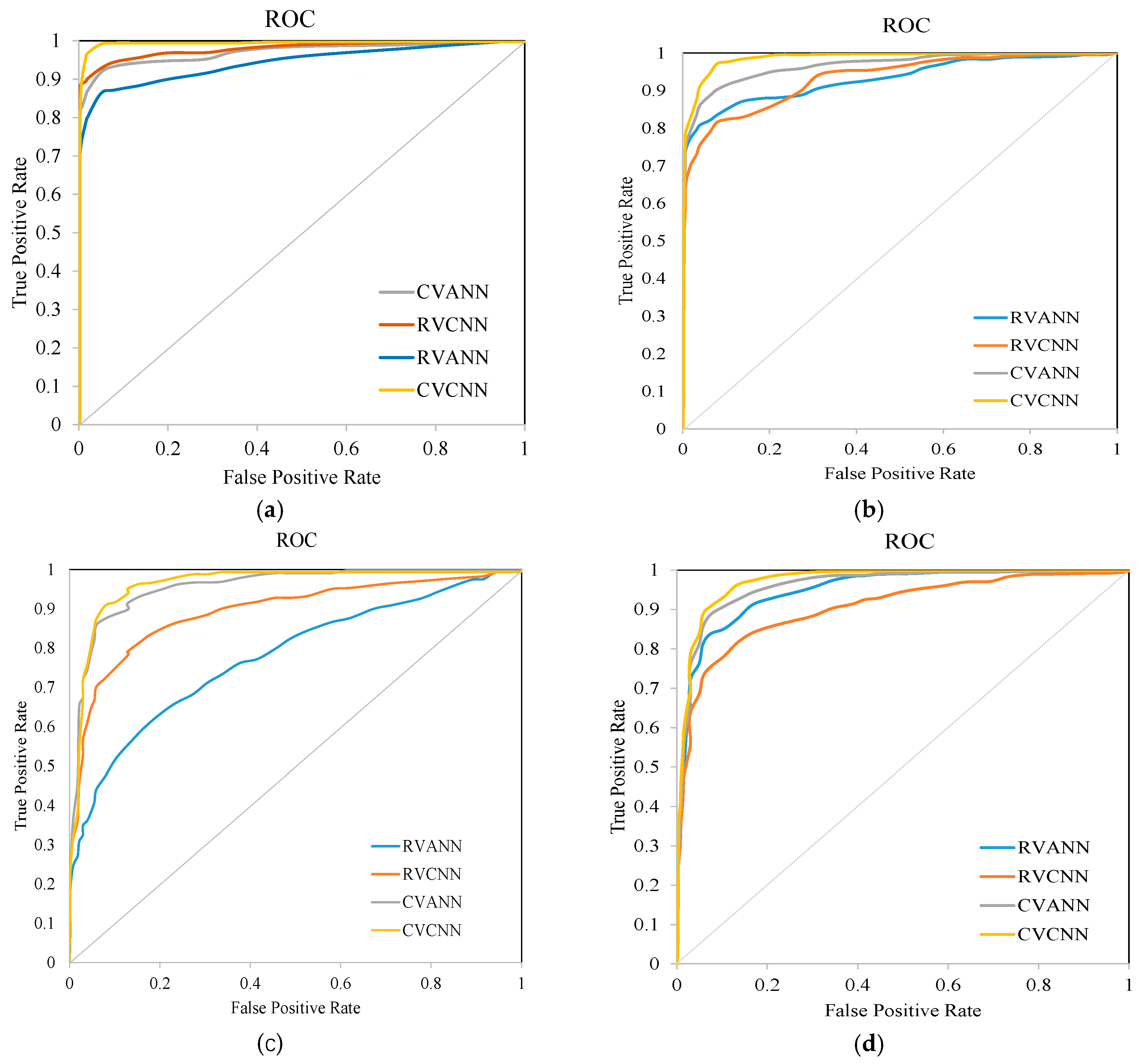
Figure 17 shows the ROC curve derived from the four study scenes by different classification algorithms when taking the best feature set F T R , F P or F T C , F P as the input. It can be observed that while the curves of all models tend to the upper left, the performance of CVCNN is significantly higher than the other modes. On the Radarsat-2 dataset, RVCNN achieved the second-best performance, while for the SIR-C dataset, CVANN ranked as second. RVANN tends to have the lowest performance in the majority cases, except for p.n. 49939.

4. Discussions

Experiments conducted on Radarsat-2 and SIR-C fully polarimetric SAR images proved the CVCNN algorithm proposed in this paper can realize high-precision oil spill classification. Following are some key findings and discussion about their main significance:
(1) In the comparison between the complex-valued model and the real-valued model, the classification performance of complex-valued models is generally better. This suggests that the complex-valued model can make better use of the polarimetric information contained in SAR data to help distinguish between mineral oil slick and biological oil film.
(2) In the comparison between ANN and CNN-based models, CNN-based models achieved relatively higher accuracy. The reason can be attributed to the fact that the CNN-based models can effectively extract texture and semantic information from SAR images and improve the integrity of the targets while suppressing the misclassification caused by speckle noise.
(3) Introducing the scattering mechanism-based features, the classification accuracy of sea oil spill models was significantly improved, and the misclassification rate of biological oil film and mineral oil slick was significantly reduced. These results demonstrated the scattering mechanism-based polarimetric features carry the key information to distinguish the mineral oil slick from the biological oil film, which is helpful to the accurate classification of the oil spill.

5. Conclusion

In this paper, a complex-valued neural network framework was proposed for marine oil spill classification. A comprehensive analysis was conducted on four typical study cases acquired by RS-2 and SIR-C to evaluate the key contribution of different factors in distinguishing clean sea water, mineral oil slick, and their biogenic look-alikes. Experimental results demonstrated that the polarimetric scattering mechanism-based features, complex-valued framework, and CNN structure all contribute to the improvement of oil spill classification performance to a certain degree. Among them, introducing the scattering mechanism-based features resulted in the largest improvement. The overall accuracy of Radarsat-2 data reached up to 94.86%, and the maximum accuracy of SIR-C images with relatively large noise impact was 90.79%, 80.81%, and 84.97% respectively. This result shows that the complex-valued network model has strong practical application potential in the detection and identification of offshore oil spills. These findings may lay a foundation for the design and implementation of polarimetric SAR-based marine oil spill classification systems.
In future work, more sophisticated models will be established given further sufficient polarimetric SAR training samples, to better explore the potential of CVCNN in marine oil spills classification, as well as other related remote sensing applications.

Acknowledgments

This work was supported in part by the National Key Research and Development Program of China (2021YFA0715101), and the Natural Science Foundation of China (42376178).

References

  1. Dong, Y.; Liu, Y.; Hu, C.; MacDonald, I.R.; Lu, Y. Chronic oiling in global oceans. Science 2022, 376, 1300-1304. [CrossRef]
  2. Marangoni, C. Sul principio della viscosita’ superficiale dei liquidi stabilito dalsig. J. Plateau. Nuovo Cim. Il Nuovo Cimento 1871, 5, 239-273.
  3. Migliaccio, M.; Gambardella, A.; Tranfaglia, M. SAR Polarimetry to Observe Oil Spills. IEEE Transactions on Geoscience and Remote Sensing 2007, 45, 506-511.
  4. Migliaccio, M.; Tranfaglia, M. A study on the use of SAR polarimetric data to observe oil spills. Europe Oceans 2005 2005, 1, 196-200.
  5. Migliaccio, M.; Ferrara, G.; Gambardella, A.; Nunziata, F. A new stochastic model for oil spill observation by means of single-look SAR data. In IEEE US/EU Baltic International Symposium, Klaipeda, Lithuania, 23-26 May 2006.
  6. Nunziata, F.; Migliaccio, M.; Gambardella, A. Pedestal height for sea oil slick observation. IET radar, sonar & navigation 2011, 5, 103-110. [CrossRef]
  7. Migliaccio, M.; Nunziata, F.; Gambardella, A. On the co-polarized phase difference for oil spill observation. International Journal of Remote Sensing 2009, 30, 1587-1602. [CrossRef]
  8. Skrunes, S.; Brekke, C.; Eltoft, T.; Kudryavtsev, V. Comparing near-coincident C-and X-band SAR acquisitions of marine oil spills. IEEE Transactions on Geoscience and Remote Sensing 2014, 53, 1958-1975. [CrossRef]
  9. Wang, W.; Lu, F.; Wu P.; Wang, J. Oil spill detection from polarimetric SAR image. In IEEE 10th International Conference on Signal Processing Proceedings, Beijing, China, 24-28 Oct. 2010.
  10. De Laurentiis, L.; Jones, C. E.; Holt, B.; Schiavon, G.; Del Frate, F. Deep learning for mineral and biogenic oil slick classification with airborne synthetic aperture radar data. IEEE Transactions on Geoscience and Remote Sensing 2020, 59, 8455-8469. [CrossRef]
  11. Song, D.; Zhen, Z.; Wang, B.; Li, X.; Gao, L.; Wang, N.; Xie, T.; Zhang, T. A novel marine oil spillage identification scheme based on convolution neural network feature extraction from fully polarimetric SAR imagery. IEEE Access 2020, 8, 59801-59820. [CrossRef]
  12. Zhang, J.; Feng, H.; Luo, Q.; Li, Y.; Wei, J.; Li, J. Oil spill detection in quad-polarimetric SAR Images using an advanced convolutional neural network based on SuperPixel model. Remote Sensing 2020, 12, 944. [CrossRef]
  13. Trabelsi, C.; Bilaniuk, O.; Zhang, Y.; Serdyuk, D.; Subramanian, S.; Santos, J.F.; Mehri, S.; Rostamzadeh, N.; Bengio, Y.; Pal, C.J. Deep complex networks. In 6th International Conference on Learning Representations (ICLR 2018), Vancouver, BC, Canada, Apr 30th through May 3rd, 2018.
  14. Zhang, Z.; Wang, H.; Xu, F.; Jin Y.Q. Complex-valued convolutional neural network and its application in polarimetric SAR image classification. IEEE Transactions on Geoscience and Remote Sensing 2017, 55, 7177-7188. [CrossRef]
  15. Li, Y.; Yang, J.; Yuan, Z.; Zhang, Y. Marine Oil Spills Detection and Classification from Polsar Images Based on Complex-Valued Convolutional Neural Network. In IGARSS 2022 - 2022 IEEE International Geoscience and Remote Sensing Symposium, Kuala Lumpur, Malaysia, 17-22 July 2022.
  16. Cloude, S. R.; Pottier, E. An entropy based classification scheme for land applications of polarimetric SAR. IEEE transactions on geoscience and remote sensing 1997, 35, 68-78. [CrossRef]
  17. Buono, A.; Nunziata, F.; de Macedo, C.R.; Velotto, D.; Migliaccio, M. A sensitivity analysis of the standard deviation of the copolarized phase difference for sea oil slick observation. IEEE Transactions on Geoscience and Remote Sensing 2018, 57, 2022-2030. [CrossRef]
  18. Nunziata, F.; Migliaccio, M.; Li, X. Sea oil slick observation using hybrid-polarity SAR architecture. IEEE Journal of Oceanic Engineering 2014, 40, 426-440. [CrossRef]
  19. Nunziata, F.; Migliaccio, M.; Gambardella, A. Pedestal height for sea oil slick observation. IET radar, sonar & navigation 2011, 5, 103-110. [CrossRef]
  20. Truong-Loi, M. L.; Dubois-Fernandez, P.; Freeman, A.; Pottier, E. The conformity coefficient or how to explore the scattering behaviour from compact polarimetry mode. In 2009 IEEE Radar Conference, Pasadena, CA, USA, 4-8 May 2009.
  21. Zhang, B.; Perrie, W.; Li, X.; Pichel, W. G. Mapping sea surface oil slicks using RADARSAT-2 quad-polarization SAR image. Geophysical Research Letters 2011, 38, L10602. [CrossRef]
  22. Skrunes, S.; Brekke, C.; Eltoft, T.; Kudryavtsev, V. Comparing near-coincident C-and X-band SAR acquisitions of marine oil spills. IEEE Transactions on Geoscience and Remote Sensing 2014, 53, 1958-1975. [CrossRef]
  23. Skrunes, S.; Brekke, C.; Eltoft, T. Characterization of marine surface slicks by Radarsat-2 multipolarization features. IEEE Transactions on Geoscience and Remote Sensing 2013, 52, 5302-5319. [CrossRef]
  24. Fortuny-Guasch, J. Improved oil slick detection and classification with polarimetric SAR. In Applications of SAR Polarimetry and Polarimetric Interferometry, Frascati, Italy, 14-16 January 2003.
  25. Spolaôr, N.; Cherman, E. A.; Monard, M. C.; Lee, H. D. ReliefF for multi-label feature selection. In 2013 Brazilian Conference on Intelligent Systems, Fortaleza, Brazil, 19-24 Oct. 2013.
Figure 1. Network structure of: (a) RVANN; (b) RVCNN.
Preprints 109497 g001
Figure 2. Network structure of CVCNN [13].
Preprints 109497 g002
Figure 3. The complex-valued convolution operation.
Preprints 109497 g003
Figure 4. The overall flowchart of this study.
Preprints 109497 g004
Figure 5. (a) PauliRGB image of the Radarsat-2 data, (b) VV power image of the Radarsat-2 data and Ground truth label marking, red represents marine oil, blue represents sea water, cyan represents biogenic oil, (c) Three scenes of SIR-C data, in which the red box indicates the region of interest considered in the experiment.
Preprints 109497 g005
Figure 6. Features extracted from the RASARSAT-2 data. (a) S V V 2 , (b) PH, (c) Cor_Co, (d) Conf_Co, (e) Conf_Co, (f) CPD-std, (g) Chi, (h) Alpha, (i) H. The S V V 2 is normalized between 0 to 1.
Preprints 109497 g006
Figure 7. Pearson correlation coefficients of SAR polarimetric features for the four study cases. (a) Radarsat-2, (b) p.n. 44327, (c) p.n. 11588, (d) p.n. 49939.
Preprints 109497 g007
Figure 8. The importance of the polarimetric features derived by ReliefF algorithm.
Preprints 109497 g008
Figure 9. The basic structure of the RVCNN and CVCNN models employed in this study.
Preprints 109497 g009
Figure 10. Classification results derived by RVANN and CVANN. (a) Enlarged view of area 1 in Fig.(b); (b) F T R : RVANN (c) Zoomed in view of area 2 in Fig.(b); (d) Zoomed in view of area 1 in Fig.(e), (e) F T C :   CVANN, (f) Zoomed in view of area 2 in Fig.(e). ([Feature set]: Classification Model).
Preprints 109497 g010
Figure 11. Classification results derived by RVCNN and CVCNN. (a) Zoomed in view of area 1 in (b), (b) F T R :   RVCNN, (c) Zoomed in view of area 2 in Fig.(b); (d) Zoomed in view of area 1 in (e), (e) F T C : CVCNN, Zoomed in view of area 2 in (e). ([Feature set]: Classification Model).
Preprints 109497 g011
Figure 12. Classification results derived by RVANN and CVANN by inputting combined feature sets. (a) Enlarged view of area 1 in Fig. (b), (b) F T R , F P : RVANN, (c) Enlarged view of area 2 in Fig.(b), (d) Enlarged view of area 1 in Fig.(e), (e) F T C , F P : CVANN, (f) Enlarged view of area 2 in Fig.(e). ([Feature set]: Classification Model).
Preprints 109497 g012
Figure 13. Classification results derived by RVCNN and CVCNN by inputting combined feature sets. (a) Zoomed in view of area 1 in Fig.(b), (b) F T R , F P : RVCNN, (c) Zoomed in view of area 2 in Fig.(b); (d) Zoomed in view of area 1 in Fig.(e), (e) F T C , F P : CVCNN, (f) Enlarged view of area 2 in Fig.(e). ([Feature set]: Classification Model).
Preprints 109497 g013
Figure 14. Classification results on p.n. 44327 oil spill data. (a) VV2 Intensity image, (b) F T R :RVANN, (c) F T C :CVANN, (d) F T C :CVCNN, (e) F T R :RVCNN, (f)  F T R , F P :RVANN, (g) F T C , F P :CVANN, (h) F T R , F P :RVCNN, (i) F T C , F P :CVCNN. ([Feature set]: Classification Model).
Preprints 109497 g014
Figure 15. Classification results on p.n. 11588 Biogenic slicks data. (a) VV2 Intensity image, (b) F T R :RVANN, (c) F T C :CVANN, (d) F T C :CVCNN, (e) F T R :RVCNN, (f)  F T R , F P :RVANN, (g) F T C , F P :CVANN, (h) F T R , F P :RVCNN, (i) F T C , F P :CVCNN. ([Feature set]: Classification Model).
Preprints 109497 g015
Figure 16. Classification results on p.n. 49939 oil spill data. (a) VV2 Intensity image, (b) F T R :RVANN, (c) F T C :CVANN, (d) F T C :CVCNN, (e) F T R :RVCNN, (f)  F T R , F P :RVANN, (g) F T C , F P :CVANN, (h) F T R , F P :RVCNN, (i) F T C , F P :CVCNN. ([Feature set]: Classification Model).
Preprints 109497 g016
Figure 17. Receiver operating curve of the classification results derived by. (a) Radarsat-2; (b) p.n. 44327; (c) p.n. 11588; (d) p.n. 49939.
Preprints 109497 g017
Table 1. J-S Divergence between PolSAR features extracted from different target pairs (Radarsat-2).
Feature J-S Divergence
S V V 2 PH Cor_Co Conf_Co Coh CPD-std Chi Alpha H
Mineral oil-Biogenic film 0.6072 0.7103 0.7197 0.6994 0.6641 0.2464 0.0056 0.7905 0.8381
Mineral-Water 0.7028 0.7355 0.7609 0.7824 0.8057 0.3109 0.1287 0.9162 0.8646
Water 0.7359 0.8915 0.8271 0.8001 0.8582 0.0035 0.1662 0.9080 0.8587
Table 2. PolSAR Features Evaluation based on J-S Divergence (SIR-C).
Feature processing number J-S Divergence
S V V 2 PH Cor_Co Conf_Co Coh CPD-std Chi Alpha H
Mineral oil-Water p.n. 44327 0.8087 0.8376 0.7969 0.6571 0.9011 0.6144 0.1287 0.8948 0.9115
p.n. 11588 0.6045 0.6701 0.7033 0.5988 0.6591 0.1057 0.0087 0.6162 0.6693
p.n. 49939 0.6188 0.7694 0.8057 0.7649 0.8588 0.5035 0.0377 0.7909 0.9018
Table 3. Implementation details of the CNN models.
Parameter Settings
Software Platform Matlab (R2022a)
Epoch 100
Learning Rate 0.01
Batch Size 100
Table 6. Comparisons of OA (%) on Radarsat-2 dataset derived by various feature inputs and classifiers.
CVCNN RVCNN CVANN RVANN
F T C 91.52 - 83.29 -
F T R - 87.15 - 80.21
F T C , F P 94.86 - 92.29 -
F T R , F P - 91.53 - 87.89
Table 7. Comparisons of OA (%) on p.n. 44327 dataset derived by various feature inputs and classifiers.
CVCNN RVCNN CVANN RVANN
F T C 87.20 - 86.69 -
F T R - 86.55 - 85.09
F T C , F P 90.79 - 88.93 -
F T R , F P - 90.16 - 88.61
Table 8. Comparisons of OA (%) on p.n. 11588 dataset derived by various feature inputs and classifiers.
CVCNN RVCNN CVANN RVANN
F T C 75.41 - 74.87 -
F T R - 73.80 - 73.46
F T C , F P 80.81 - 79.94 -
F T R , F P - 79.48 - 77.51
Table 9. Comparisons of OA (%) on p.n. 49939 dataset derived by various feature inputs and classifiers.
CVCNN RVCNN CVANN RVANN
F T C 82.59 - 81.93 -
F T R - 81.78 - 73.79
F T C , F P 84.97 - 82.89 -
F T R , F P - 84.66 - 78.11
Disclaimer/Publisher’s Note: The statements, opinions and data contained in all publications are solely those of the individual author(s) and contributor(s) and not of MDPI and/or the editor(s). MDPI and/or the editor(s) disclaim responsibility for any injury to people or property resulting from any ideas, methods, instructions or products referred to in the content.
Copyright: This open access article is published under a Creative Commons CC BY 4.0 license, which permit the free download, distribution, and reuse, provided that the author and preprint are cited in any reuse.
Prerpints.org logo

Preprints.org is a free preprint server supported by MDPI in Basel, Switzerland.

Subscribe

© 2024 MDPI (Basel, Switzerland) unless otherwise stated