CWT-AM-CNN: A Lightweight Feature Extraction Network with Attention Mechanism Based on CWT Peak Seeking Method for Aero-Engine Hot Jet FT-IR Classification

Focusing on the problem of identifying and classifying aero-engine models, this paper measures the infrared spectrum data of aero-engine hot jets using a telemetry Fourier transform infrared spectrometer. Simultaneously, infrared spectral data sets with the six different types of aero-engines are created. For the purpose of classifying and identifying infrared spectral data, a CNN architecture based on the continuous wavelet transform peak seeking attention mechanism (CWT-AM-CNN) is suggested. This method calculates the peak value of middle wave band by continuous wavelet transform, and the peak data is extracted by the statistics of the wave number locations with high frequency. Attention mechanism is used for the peak data, and the attention mechanism is weighted to the feature map of the feature extraction block. The training set, vali-dation set and prediction set are divided in the ratio of 8:1:1 for the infrared spectral data sets. For three different data sets, CWT-AM-CNN proposed in this paper is compared with the classical classifier algorithm based on CO2 feature vector and the popular AE, RNN and LSTM spectral processing networks. The prediction accuracy of the proposed algorithm in the three data sets is as high as 97%, and the lightweight network structure design not only guarantees high precision, but also has a fast running speed, which can realize the rapid and high-precision classification of the infrared spectral data of the aero-engine hot jets.

Keywords:

Subject: Engineering - Aerospace Engineering

1. Introduction

Aircraft fault detection requires rapid identification of aero-engine models, and infrared spectroscopy provides a solution. A method for determining a substance's chemical makeup and molecular structure is called infrared spectroscopy (IR) [1,2,3]. This method measures the wavelength and intensity of the absorbed or emitted light and generates a particular spectrum diagram by taking advantage of the energy level transition that occurs in material molecules when exposed to infrared radiation. Therefore, the chemical bond and structure of the substance are analyzed and judged. This technology been studied importantly in environmental monitoring [4], refuse classification [5], biochemistry [6] and other fields.

Varied types of aero-engines will create varied gas compositions and emissions during combustion. The categorization features of aero-engines are frequently connected to fuel type, combustion mode, and emission characteristics. The vibrations and rotations of these molecules form a specific infrared absorption and emission spectrum. Fourier Transform Infrared Spectrometer (FT-IR Spectrometer) [7,8,9] is an important means to measure infrared spectrum. Interferogram is obtained through interferometer. Based on Fourier transform, the interferogram is reduced to spectrogram. In this paper, FT-IR is used to cover a wider spectral range(The spectral range of the hyperspectrum is usually from the visible region (0.4-0.7µm) to the short-wave infrared (SWIR) region (nearly 2.4µm), and the spectral coverage of the FT-IR spectrometer used in this experiment is 2.5~12µm.) and the spectral data implies molecular type and structure information, so the richer and finer characteristic information of FT-IR is the data basis for classification and recognition in this paper. At the same time, hyperspectral detection usually uses a dispersive spectrometer to measure the continuous narrow-band spectrum in the visible region. Different from hyperspectral detection, FT-IR has a larger luminous flux. This method can complete the interferometer measurement of optical signals in the range of 2.5~12µm and convert them into spectral data in a few seconds. Since passive FT-IR can gather data in any direction and perform fast target analysis as well as continuous, long-distance real-time monitoring, it is frequently employed to identify air contaminants. This method is more suitable for the measurement of the hot jet spectrum of aero-engines.

The research on image recognition methods has been mature [10,11]. While, for spectral data classification methods, spectral classification methods of hyperspectral data provide us with a reference approach, which is divided into classical methods and deep methods. Li[12] summarized that the classical method of spectral classification is to transform data into new feature space and retain identification information through data projection, including principal component analysis (PCA), independent component analysis (ICA), linear discriminant analysis (LDA), one-dimensional discrete wavelet transform (1D-DWT), etc. With the rapid development of deep learning in recent years, various feature extraction frameworks have emerged in an endless stream. Deep learning methods for spectral classification mainly include convolutional neural network (CNN), recurrent neural network (KNN), Transformer[13] and variants of the above methods. AUDEBERT[14], RASTI[15] summarized that deep learning methods mainly include supervised learning methods (1DCNN, RNN, recursion and convolution) and unsupervised learning methods (AE and PCA). For the method of spectral feature extraction in deep learning networks, Lu[16] adopted five convolutional layers 1DCNN, Chen[17] and Kemker[18] adopted automatic encoder (AE) and stacked autoencoder (SAE), Ding [19] adopted graph convolutional network, Li[20] combined spectral convolution and dictionary learning. Ashraf[21] constructed BERT induction, and Hamouda[22] used spectral digits and minimum redundancy and maximum correlation selection. Transformer framework structure is the most popular deep learning structure at present, and it is also a popular research topic in hyperspectral data processing in recent years. However, Transformer replaces computing efficiency with high memory consumption, which needs to take up more memory resources and does not match the computing power of edge computing platform. In contrast, lightweight network design is needed for our infrared spectral data to achieve a balance between accuracy and efficiency. The wide application of 1DCNN in spectral feature extraction and appropriate memory and time efficiency make 1DCNN the preferred choice for the network structure in this paper.

Because of the extraordinary lack of public data sets, the infrared spectral data of six different models of aero-engine hot jets are measured by outfield experiment and three spectral data sets are made according to the measurement distance and the different environment. In this paper, a convolutional neural network framework based on continuous wavelet transform peak seeking attention mechanism is designed for the extraction of spectral features and the realization of multi-classification tasks. In order to compare the accuracy of the deep learning method and the traditional classification algorithm, this paper designs the characteristic spectral vector based on CO₂, an important component of the aero-engine hot jet, and combines it with the classifier to compare the classification accuracy of CWT-AM-CNN with the traditional classifier method. To compare the effectiveness of deep learning method of spectral data, CWT-AM-CNN is compared with the popular AE, RNN and LSTM spectral processing networks.

The contribution of this paper is summarized in the following three points:

This paper utilizes the infrared spectrum detection method of aero-engine hot jet as the foundation for aero-engine identification and input of data source. The hot jet is a significant infrared radiation feature of an aero-engine, and the infrared spectrum offers molecular-level information about substances. Thus, employing this approach for categorization is more scientifically valid.
In this paper, a new benchmark data set is developed. The data set is obtained from the field environment. The dataset consists of three sub-datasets, including a 443 spectral data set with a resolution of 1cm⁻¹, a 1371 spectral data set with 1cm⁻¹ and 0.5cm⁻¹ resolution and a large dataset of 1814 spectral data. The data set covers the infrared spectrum in the wavelength range of 2.5~12 μm, including six types of different aero-engine models (including turbine engine and turbofan engine).
This paper provides a deep learning framework for classification of aero-engine hot jet infrared spectra. A convolutional neural network based on peak seeking attention mechanism is designed. The backbone network consists of three feature extraction blocks with the same structure, batch normalization layer and maximum pooling layer. In the part of attention mechanism based on peak seeking, the spectral peak value is detected by continuous wavelet transform method and the peak wave number of high frequency occurs is counted. The attention mechanism weights the peak value obtained by statistics and acts on the feature map of the trunk CNN. The structure of the network is light, and the classification accuracy and operation efficiency can be taken into account.

The structure of this paper consists of five parts. The first section reviews the method of spectral feature extraction, and briefly describes the method, contribution and structure of this paper. In the second section, the detailed structure and algorithm details of the attention mechanism convolutional neural network designed in this paper are described. In the third section, the data set used in the experiment is designed, and the design of the outfield experiment, the data preprocessing and the composition of the spectral data set are described in detail. In the fourth section, the experiment and results are analyzed, and the performance results are used to evaluate and analyze the experiment, and the traditional classifier methods and the current popular spectral processing network methods are compared. The fifth section summarizes the thesis.

2. Spectral Classification Network Structure Design

In this section, the CNN based on peak seeking attention mechanism designed by infrared is described, which consists of four parts: overall network structure design, backbone network design, peak-based attention mechanism and network training method.

2.1. Overall Network Design

Convolutional Neural Networks (CNNs) structures commonly used at present include LeNet-5[23], AlexNet[24], VGG[25], GoogleNet[26], ResNet[27], etc., all of which achieve high accuracy in the classification of ImageNet data sets. However, the commonality feature of these algorithms is that by increasing the depth of the network, the accuracy of the calculation results is exchanged with more excessive consumption of computing resources. Our spectral data adopts the file type of prn, which is expressed as two-dimensional point set data of horizontal wave number and vertical brightness temperature spectrum. The data are characterized by a single piece of data with many data points and few dimensions. Choosing a network model that is too deep will reduce the efficiency of the algorithm and consume a lot of computing resources. In hyperspectral spectral processing, 1DCNN is often used as the extraction method of spectral data features, so we design a spectral classification network with 1DCNN as the basic structure of spectral data processing.

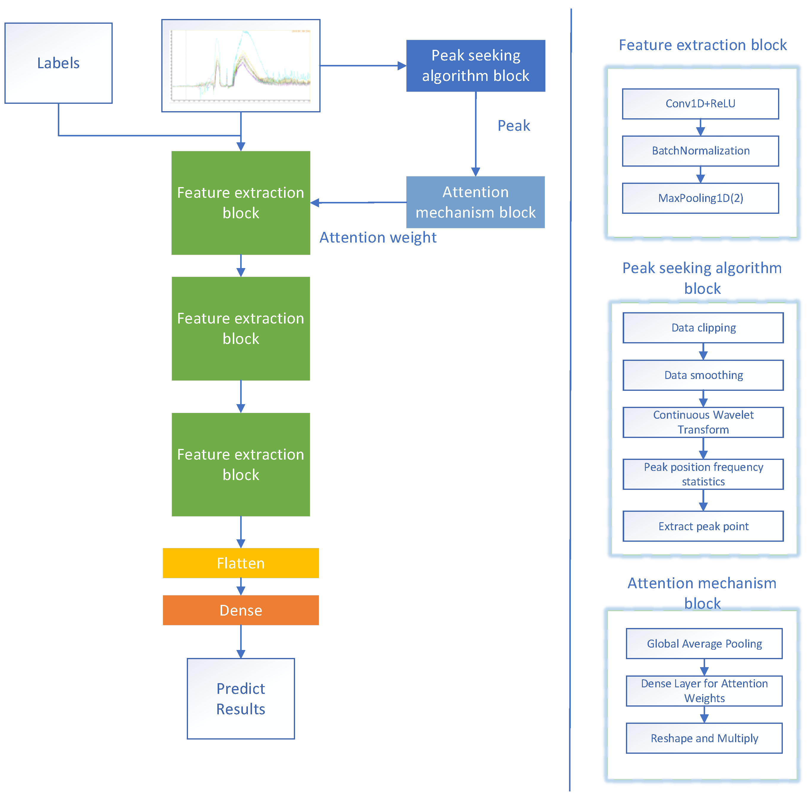
The CWT-AM-CNN developed in this paper, as depicted in Figure 1, is composed of three modules: backbone network, feature extraction block, peak seeking algorithm block and attention mechanism block. When the network is in the training stage, the infrared spectrum and its label information are input, and the feature extraction block is first entered to extract the feature map. At the same time, the peak seeking block is input to detect the peak value. The peak detection results are assigned to the attention mechanism, and the attention weight is assigned to the feature map. When the network is in the prediction stage, the prediction data set is entered into the network, and the classification results and performance results are obtained.

2.2. Backbone Network Design

Before data entry, we need to unify the spectral data with different resolutions, because the aero-engine hot jet is composed of high-temperature gas, and the radiation characteristics of high-temperature gas are more obvious in the medium-wave band (400-4000cm⁻¹), so we focus on cutting the data in the medium-wave band. The 0.5 cm⁻¹ resolution data are downsampled and data amounts in the mid-wave band are adjusted to ensure the consistency of the model data input.

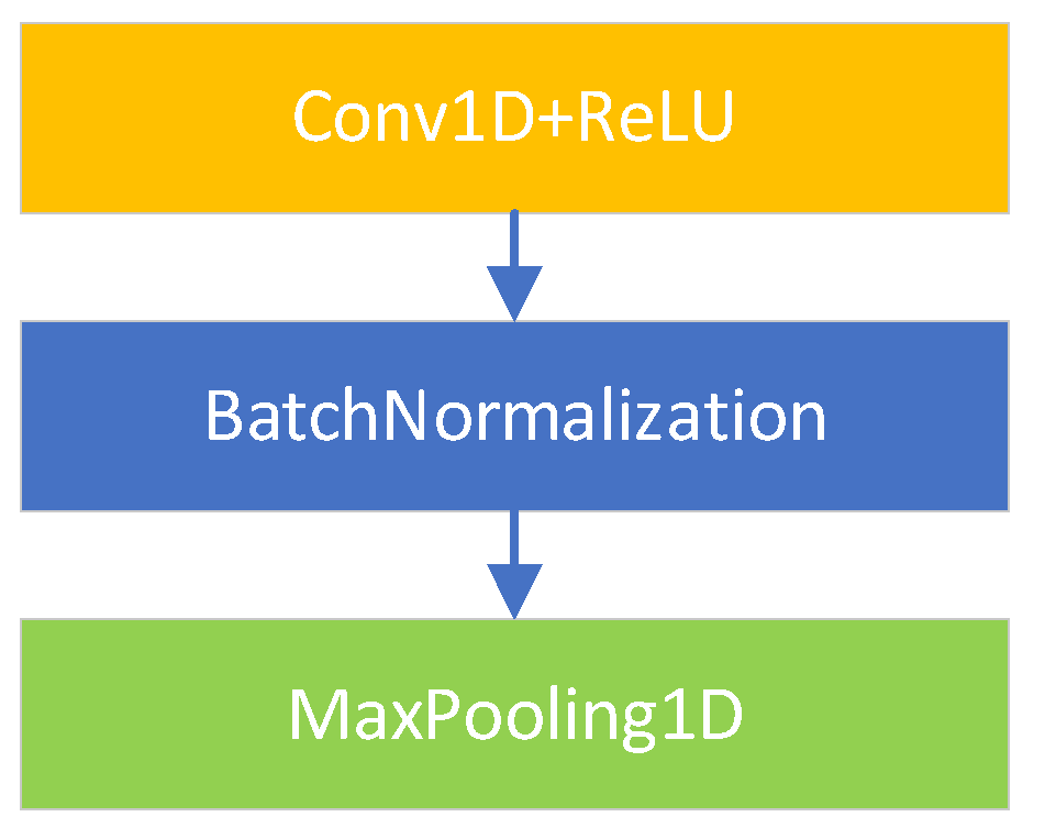
We define the three components of the backbone network as feature extraction blocks. Each feature extraction block, as presented in Figure 2, consists of one-dimensional convolution layer, Batch Normalization layer and Maximum pooling layer.

①One-dimensional convolutional layer (Cov1D layer): The convolutional layer is a means of feature extraction for convolutional neural networks, and the convolutional layer is complete with linear and translation invariant operations. Through convolution operation, we can extract the features of the data, enhance some features of the original signal, and reduce the noise.

The convolution between two functions can be defined as

f, g : R^{d} \to R

(f * g) (x) = \int f (z) g (x - z) d z

(1)

Convolution can be understood as the overlap between two functions when the function is flipped and shifted by x. For two-dimensional tensors, convolution can be written as:

(f * g) (i, j) = \sum_{a} \sum_{b} f (a, b) g (i - a, j - b)

(2)

Among them,

(a, b)

is the index of

f

，

(i - a, j - b)

is the index of

g

②Batch Normalization(BN)[28] is commonly used to accelerate convergence and solve the gradient dispersion of deep neural networks. The BN layer can be represented as a learnable network layer with parameters(γ、β).With the introduction of BN, the network can learn to recover the feature distribution that the original network needs to learn.

Assuming that the input from a small batch

B

x \in B

, BN can be converted to

x

according to formula (3):

B N (x) = γ ⊙ \frac{x - {\hat{μ}}_{B}}{{\hat{σ}}_{B}} + β

(3)

Among them,

{\hat{μ}}_{B}

is the sample mean of the small lot

B

{\hat{σ}}_{B}

is the sample standard deviation of the small lot

B

. After applying BN, the mean value of the generated small batches is 0 and the unit variance is 1.

γ

is the scale parameter, while

β

is the shift parameter. These two parameters need to be learned.

BN maintains the amplitude of change in the middle layer during training, through the active centralization of each layer. While adjust the mean and size by re-adjusting

{\hat{μ}}_{B}

and

{\hat{σ}}_{B}^{2}

, can help smooth the middle layer change. The

{\hat{μ}}_{B}

and

{\hat{σ}}_{B}^{2}

are shown in equation (4):

\begin{matrix} {\hat{μ}}_{B} & = \frac{1}{| B |} \sum_{x \in B} x \\ {\hat{σ}}_{B}^{2} & = \frac{1}{| B |} \sum_{x \in B} {(x - {\hat{μ}}_{B})}^{2} + ϵ \end{matrix}

(4)

Where, the constant

ϵ

＞0。

BN can train the model with a larger initial learning rate to achieve fast convergence. When the convergence rate is very slow, gradient explosion, etc., BN can be used. At the same time, the use of BN behind the convolution layer can normalize the value of each spatial position.

③Maximum pooling layer: Pooling is a method of downsampling in CNN, which can reduce the amount of data processing while retaining useful information. Operations such as convolution layer, pooling layer, and activation function layer can be understood as mapping raw data to the hidden layer feature space.

④Extension layer: Splice learned feature maps.

⑤Fully Connected layer (FC layer) : The purpose of the FC layer is to transform the acquired distributed feature representation into the corresponding sample label space. The FC layer integrates the features together and outputs them as one value, which greatly reduces the influence of the feature position on the classifier.

2.3. Attention Mechanism based on Peak Seeking

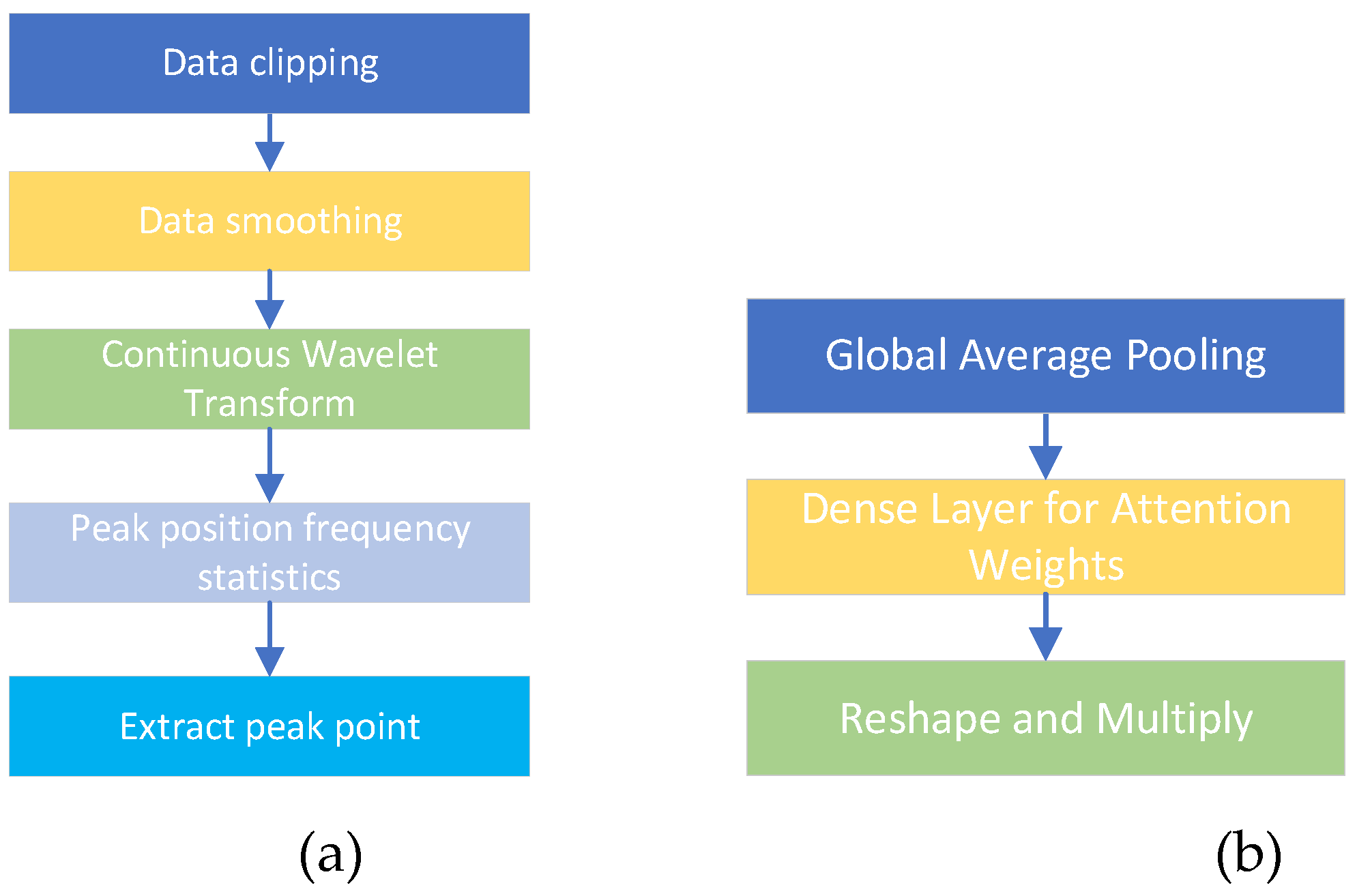
The attention mechanism based on peak seeking is mainly composed of two parts, one part is the peak seeking algorithm, the other part is the attention mechanism. The peak seeking algorithm is used to analyze the infrared spectral data in the mid-wave band. In the part of attention mechanism, peak features are input, Global Average Pooling (GAP) is added, and attention weights are calculated and applied to the feature map of the backbone network. Figure 3 shows the composition diagram of the attention mechanism module based on peak seeking. The left figure is the peak seeking algorithm block, and the right figure is the attention mechanism block.

2.3.1 Peak Seeking Algorithm Block

Continuous Wavelet Transform (CWT) is a classical peak detection method that uses wavelet transform to analyze signals at multiple scales to detect peaks at different scales.

The continuous wavelet coefficient

W (a, b)

is calculated as follows:

W (a, b) = \int_{- \infty}^{\infty} x (t) Ψ^{*} (\frac{t - b}{a}) d t

(5)

Where,

x (t)

is the original signal, which is generally the continuous time signal,

Ψ (t)

represents the complex conjugate of the wavelet function, the scaling parameter

a

is used to control the broadening or compression of the wavelet function in time and frequency, and the translation parameter

b

is used to control the translation of the wavelet function in time. This formula is the result of the transformation of the original signal with the wavelet function under different scales and translations.

We describe the algorithm running flow of the peak seeking algorithm block in the form of pseudo-code:

Algorithm 1 : Peak seeking algorithm and peak statistics.

Input: Spectral data.

Output: Peak data.

①: Trim the mid-wave band of spectral data (400-4000cm⁻¹).
②: Data smoothing.
③: Set the threshold and scale parameters of continuous wavelet change.
④: Count the wave number with peak value.
⑤: Extract the wave number position with high frequency according to the proportion of threshold value.
⑥: According to the peak wave number position, for each data, the adjacent points are extracted as the peak data points.
⑦: Output the peak data for each spectral data.

2.3.2. Attention Mechanism

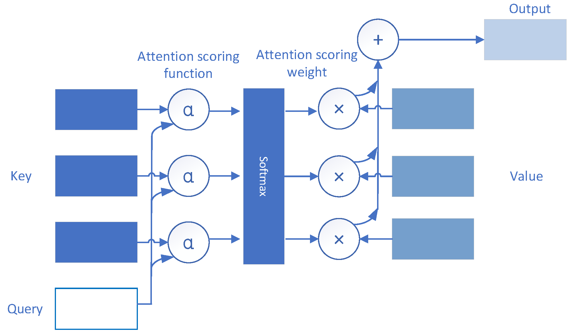
Attention Mechanism(AM) consists of three parts: Query、Key and Value. Suppose there is a query

q \in R^{q}

and M key-value pairs

(k_{1}, v_{1}), \dots, (k_{m}, v_{m})

, where

k_{i} \in R^{k}, v_{i} \in R^{v}

, the attention aggregation function is expressed as a weighted sum of values:

f (q, (k_{1}, v_{1}), \dots, (k_{m}, v_{m})) = \sum_{i = 1}^{m} α (q, k_{i}) v_{i} \in R^{v}

(6)

Among them, the attention weight (scalar) of the query

q

and key

k_{i}

is mapped into a scalar by the two vectors of the attention score function

α

, and then obtained by softmax operation:

α (q, k_{i}) = s o f t m a x (a (q, k_{i})) = \frac{\exp (a (q, k_{i}))}{\sum_{j = 1}^{m} e x p (a (q, k_{j}))} \in R

(7)

Figure 4 reflects the operation of the attention mechanism, in which attention score function is indicated

α

. Choosing different attention scoring functions

α

leads to different attention gathering operations.

We describe the action mode of the attention mechanism based on peak seeking in the network in the form of pseudo code:

Algorithm 2: CNN with attention Mechanism.

Input: Spectral data, peak data.

Output: Prediction label for prediction data set.

①: Trim the mid-wave band of spectral data (400-4000cm⁻¹)
②: The Adam optimizer with a learning rate of 0.00001 is adopted, and the number of iterations ∈ is set to 500.
③: Create a training and test data loader.
④: for i = 1 to ∈ do:
⑤: Using feature extraction block to extract shallow features from spectral data.
⑥: Global average pooling of peak data and intensive layer calculation of attention weight.
⑦: Apply the weight of attention mechanism to feature graph.
⑧: The weighted feature graph continues to extract features.
⑨: Calculate the Loss function, category and accuracy.
⑩: End for
⑪: Use trained models and data for prediction to obtain predictive labels.

2.4. Network Training Method

2.4.1. Optimizer

The optimizer is a method for finding the optimal solution of the model. The commonly used optimizer such as gradient descent(GD) method includes standard gradient descent, stochastic gradient descent (SGD), batch gradient descent (BGD), GD method is slow to train and easy to fall into the local optimal solution, and adaptive learning rate optimization algorithms, including AdaGrad, RMSProp, Adam and AdaDelta. Among them, Adam optimizer is the most commonly used, which is suitable for many kinds of neural network structures, such as CNN, RNN, GANs and so on.

Adaptive Moment Estimation (Adam)[35] uses exponential weighting to estimate momentum and second moments with winter averages. The state variables of Adam are:

\begin{matrix} v_{t} \leftarrow β_{1} v_{t - 1} + (1 - β_{1}) g_{t} \\ s_{t} \leftarrow β_{2} s_{t - 1} + (1 - β_{2}) g_{t}^{2} \end{matrix}

(8)

Where

β_{1}

and

β_{2}

are non-negative weighted parameters, the

β_{1}

usually set to

0.9

and the

β_{2}

usually set to

0.999

. Standardized state variables can be derived using the formula below:

{\hat{v}}_{t} = \frac{v_{t}}{1 - β_{1}^{t}}

(9)

{\hat{s}}_{t} = \frac{s_{t}}{1 - β_{2}^{t}}

(10)

As a result, the update formula of gradient is obtained:

g_{t}^{'} = \frac{η {\hat{v}}_{t}}{\sqrt{{\hat{s}}_{t}} + ϵ}

(11)

Where,

η

is the learning rate,

ϵ

is a constant which usually set to 10^-6.

A simple update is shown in formula 12:

x_{t} \leftarrow x_{t - 1} - g_{t}^{'}

(12)

By combining momentum and root mean square propagation (RMSProp), Adam dynamically modifies the learning rate of each parameter, and dynamically adjusts the update step of parameters in the training process, which improves the convergence speed and stability. Moreover, Adam can achieve a excellent balance between computational complexity and performance, and can ensure good performance while having low computational complexity.

2.4.2. Loss Function

The cross-entropy loss function is usually used for classification tasks, which is used to describe the difference of the sample probability distribution and to measure the difference between the learned distribution and the real distribution. The cross-entropy loss function can be expressed as:

Loss = - \frac{1}{N} \sum_{i = 0}^{N - 1} \sum_{k = 0}^{K - 1} y_{i, k} l n p_{i, k}

(13)

Where, K represents the number of tag values and N represents the number of samples, the

y_{i, k}

indicates the real label of the

i t h

sample is

k

,and

p_{i, k}

represents the probability that the sample

i

is predicted to be the

k

tag value. The smaller the value of cross entropy, the better the prediction effect of the model. At the same time, cross-entropy is often used together with softmax in classification. Softmax sums up the classification predicted values of the output results to 1, and then calculates the loss by cross-entropy.

2.4.3. Activation Function

Rectified Linear Unit (ReLU) is a commonly used nonlinear activation function. Relu controls the input of data. If the input is less than or equal to zero, the output will be zero. If the input is a positive number, the output will be the same as the input value. Relu can be expressed as:

f(x)=max(0,x)

(14)

The function of ReLU activation function is to introduce nonlinear transformation, so that the neural network has the ability to grasp more complex patterns and features. Its main advantages are that the calculation is simple, there is no gradient disappearance problem, and it can accelerate the convergence and improve the generalization ability of the model.

3 Spectral Dataset

The third section briefly describes the production process of aero-engine hot jet infrared spectral data set, including design of aero-engine spectrum measurement experiment, data preprocessing and data set production.

3.1. Design of Aero-Engine Spectrum Measurement Experiment

Initially, outfield measurement experiment were conducted to acquire infrared spectrum data from six types of aero-engines. The experiment utilized two FT-IR spectrometers: the EM27 and the telemetry FT-IR spectrometer created by the Aerospace Information Research Institute. The precise specifications of the two devices are displayed in Table 1:

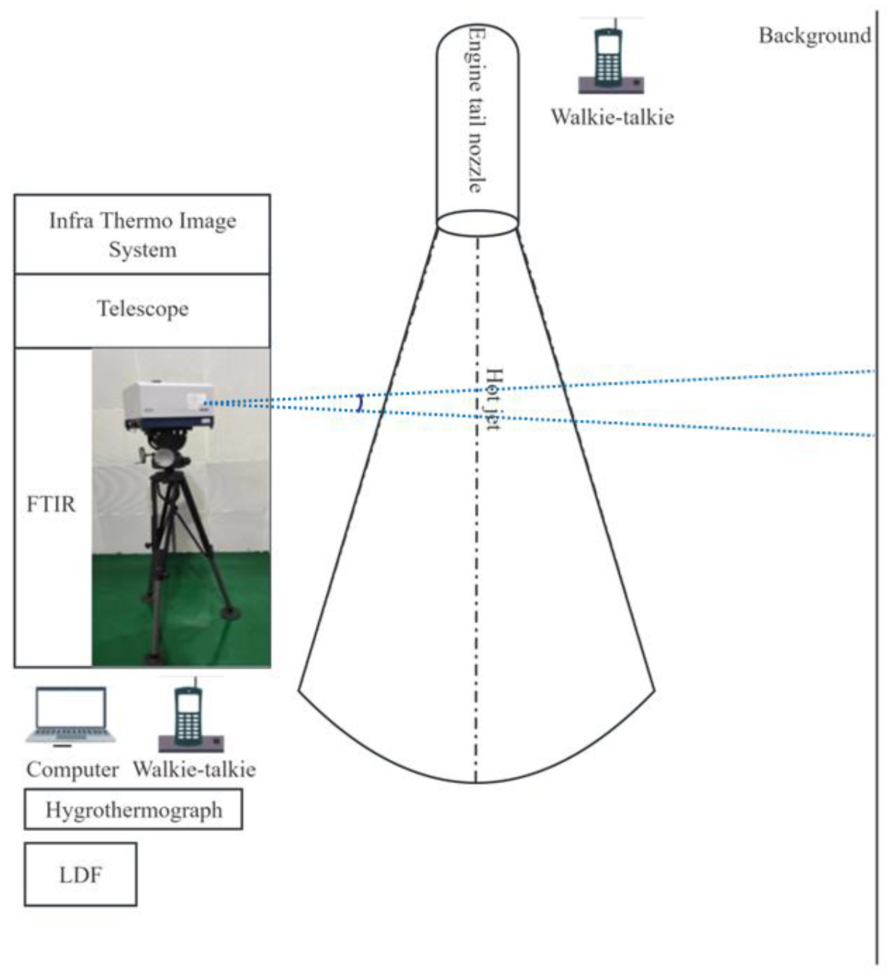
Meanwhile, the infrared spectrum measurement of aero-engine hot jet is arranged on the spot as shown in figure Figure 5:

The aero-engine hot jet is mainly composed of gases. The infrared spectrum of the hot jet measured by the outfield experiment is not only determined by the radiation of the mixed gas itself, but also a complex result of the comprehensive action of many factors. Environmental temperature, humidity and measurement distance are the influencing factors of the experiment. Thus, we recorded the parameters of environmental conditions during the experiment as shown in Table 2:

The spectrum of gas is affected by many complex factors, such as pressure, temperature, humidity and environment. Among them, the environmental temperature will affect the response of the spectrometer, resulting in the inconsistency before and after the spectrogram; the environmental humidity will affect the intensity of the spectrum and the width of the characteristic spectrum; the observation distance indicates the atmospheric transmission on the measurement path. The atmosphere will absorb and attenuate the spectrum. The transmission of solar radiation and surface thermal radiation in the atmosphere is influenced by the absorption and scattering of atmospheric molecules such as H₂O, mixed gases (CO₂, CO, N₂O, CH₄, O₂), O₃, N₂, etc., as well as the scattering or absorption of aerosolized particulate matter. This leads to a reduction in the intensity of both solar radiation and surfaces thermal radiation. When the difference between the target and our result is considerable, the atmosphere will significantly impact the acquired spectrum. Currently, we employ the method of conducting experiments in the outfield, and the distance of the experiment is relatively short. While the gas temperature of the hot jet is generally as high as 300-400 ℃, which is very different from the background, so the effects of atmosphere and environment can be ignored.

3.2 Data Preprocessing

The Brightness Temperature spectrum (BTS) [29,30] of an object refers to the temperature of a blackbody that emits the same spectral radiation intensity at the same wavelength as the object. The utilization of BTS analysis can directly extract the characteristics of the target gas.

To get the BTS using passive infrared spectrum, it is essential to subtract the instrument's bias and response from the measured spectral signal obtained by the spectrometer. This subtraction allows us to acquire the incident radiance spectrum on the spectrometer.

T (v)

can be calculated by transforming Planck’s formula to obtain the formula below:

T (v) = \frac{h c v}{k l n {[L (v) + 2 h c^{2} v^{3}] / L (v)}}

(15)

In the formula, Planck’s constant is recorded as

h

with a value of 6.62607015 × 10⁻³⁴ J·S,

c

is the speed of light with a value of 2.998 × 10⁸ m/s,

v

is the wave number in cm⁻¹,

k

is Boltzmann’s constant with a value of 1.380649 × 10⁻²³ J/K, and

L (v)

stands for the radiance about the wave number.

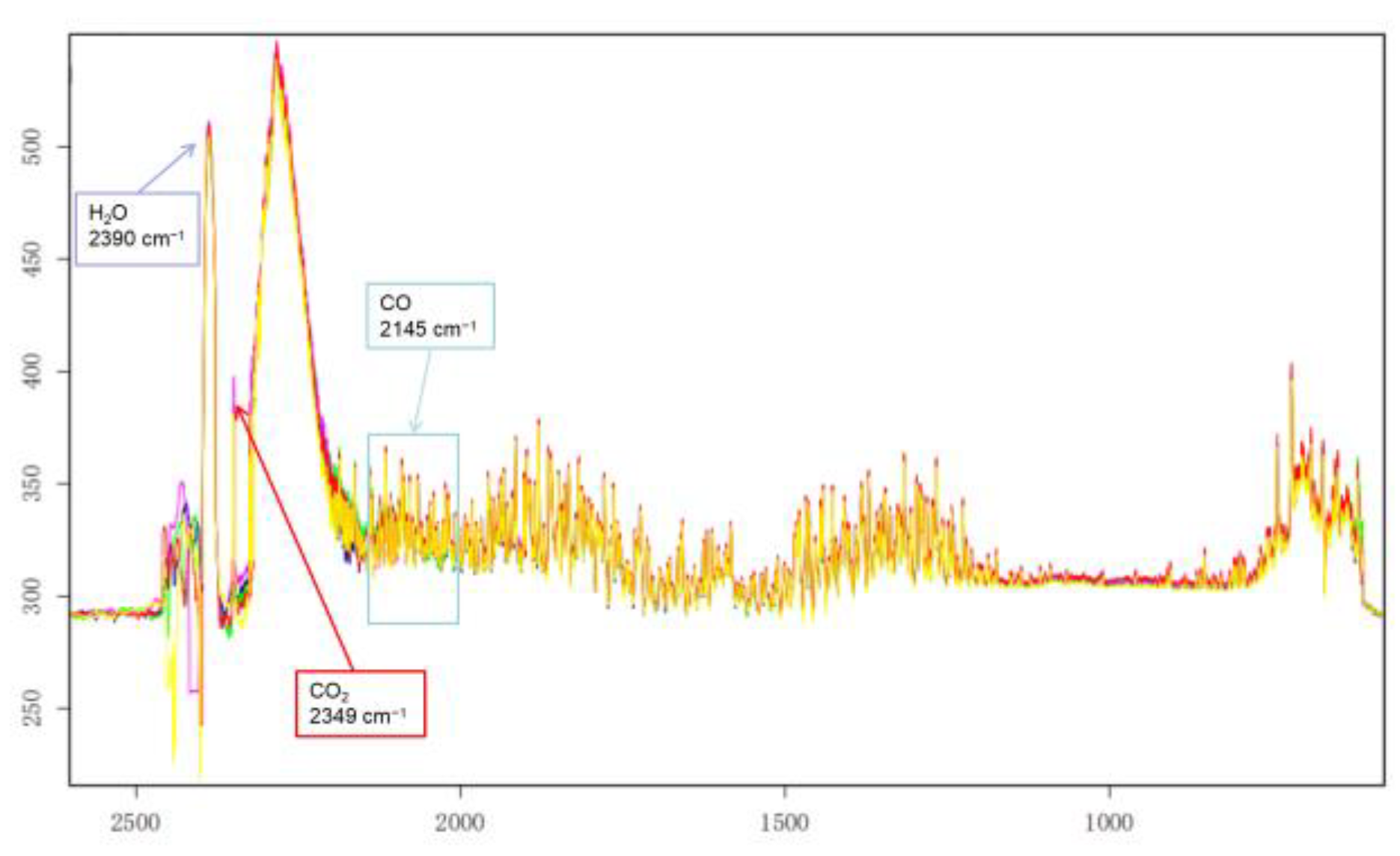
The BTSs of the aero-engine hot jets are measured experimentally as shown in Figure 6, in which the transverse coordinate is wavenumber and the longitudinal coordinate is Kelvin temperature. Simultaneously, the important components of the hot jet are marked in the Figure 6:

3.3 Data Set Production

According to the difference of test object, detection distance and detection environment, three types of data sets are made to complete the experiment of the algorithm. The specific data information is presented in Table 3, Table 4 and Table 5:

4. Experiments and Results

The fourth section continues with the experimental evaluation of the algorithm. Initially, this paper introduces the performance measures of the classification algorithm and presents the experimental results of the network on three data sets. Then the experimental results with the classifier method based on CO₂ feature vector and the method using CNN, AE, RNN and LSTM are compared. Finally, the ablation study is proved to compare the effectiveness of the peak method, the effectiveness of the attention mechanism, the design of the network and the running time.

4.1 Performance Measures and Experimental Results

The performance measures for aero-engine spectral classification include accuracy, precision, recall, F1-score and confusion matrix. If an instance is classified as a positive class and is correctly predicted as positive, it is labeled as TP. If it is predicted as negative, it is labeled as FN. Conversely, if an instance is classified as a negative class and is incorrectly predicted as positive, it is labeled as FP. If it is correctly predicted as negative, it is labeled as TN. Based on the above assumptions, these performance measures are respectively defined as follows:

①Accuracy: the ratio of correctly classified samples to the total number of samples.

Accuracy = \frac{T P + T N}{T P + T N + F P + F N}

(16)

②Precision: the ratio of the number of true positive samples to the total number of samples predicted as positive.

Precision = \frac{T P}{T P + F P}

(17)

③Recall: the ratio of the number of samples correctly predicted to be in the positive category to the number of samples in the true positive category.

Recall = \frac{T P}{T P + F N}

(18)

④F1-score: a metric that quantifies the overall performance of a model by combining the harmonic mean of precision and recall.

F 1 - score = \frac{2^{*} P^{*} R}{P + R}

(19)

where,

P

stands for the precision and

R

stands for the recall.

⑤Confusion matrix: The confusion matrix provides a comprehensive evaluation of the classifier's performance in classifying various categories. It displays the discrepancy between actual value and predicted values. The diagonal elements of the matrix indicate the number of accurate predictions generated by the classifier for each category. Table 6 displays the confusion matrix:

This research validates the efficacy of the CWT-AM-CNN method by assessing its performance on three benchmark data sets. The computation experiment is conducted on a Windows 10 workstation with a 32GB RAM, an Intel Core i7-8750H processor, and a GeForce RTX 2070 graphics card.

Specific parameters of the CWT-AM-CNN are provided by Table 7:

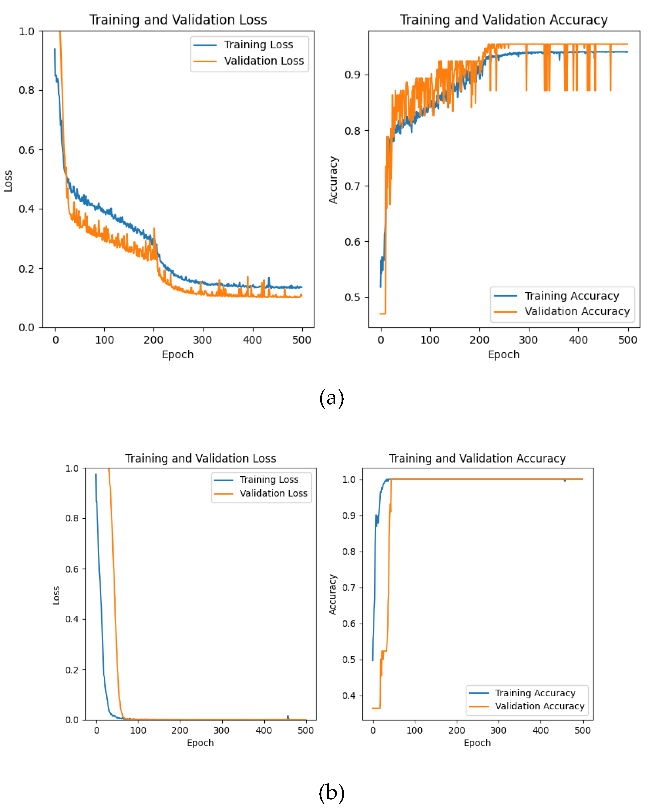
According to the table parameters, we conduct network training and label prediction, and the experimental results are displayed in Table 8:：

By analyzing the experimental results of the Loss curve and the Accuracy curve, we observe that the CWT-AM-CNN effectively enhances the processing speed of spectral data and converge rapidly in short training. In terms of accuracy, first of all, according to the overall performance of the algorithm in short training. In terms of accuracy, first of all, according to the overall performance of the algorithm in the three data sets based on Accuracy and F1-score, Accuracy is higher, indicating that the overall classification performance of the algorithm is better, and high F1-score represents a good balance performance of the classifier. Secondly, according to the analysis of the three data sets of Precision and Recall, the Precision is high, indicating that the algorithm performs well in reducing false positives, while Recall is slightly lower than Precision, indicating that the classifier still has some room for improvement in reducing false positives. According to the results of the confusion matrix, the three categories in Dataset A show that the component of the first category is relatively weak, and the other two categories have good performance; the number of data in Dataset B is relatively small, and the performance of the network on this data set is perfect, and each category is accurate; in Dataset C, the fifth category is unideal, and the classification of other categories is very accurate.

The experimental results show that the CWT-AM-CNN designed in this paper performs well on the three spectral data sets. In the process of the experiment, some exceptional cases like engine failure have remotely impact on our classification results. On the other hand, our network as a whole has good robustness, and the incorrect data has little influence on the overall classification accuracy.

4.2 Comparative Experimental Results of Traditional Classification Methods

The main components of the aero-engine hot jet are analyzed to To compare with the classical classifier method. Meanwhile, the feature vector is constructed to be used in conjunction with classifier methods. As known, the emission products of an aero-engine typically include oxygen (O₂), nitrogen (N₂), carbon dioxide (CO₂), steam (H₂O), carbon monoxide (CO), et al. 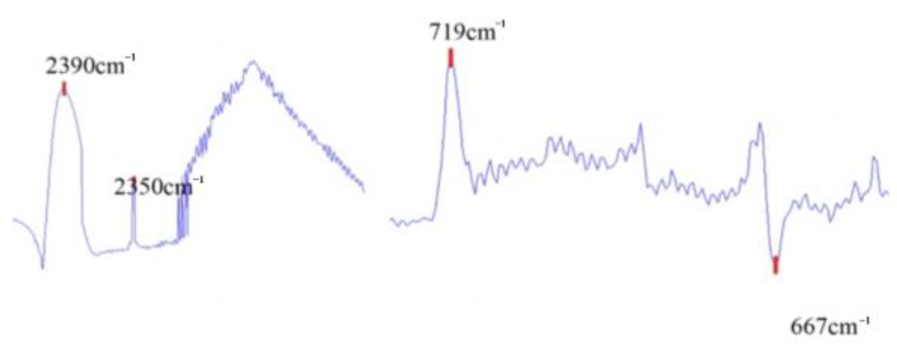Among them, the spectral characteristics of CO₂ are obvious. Based on the peak positions of CO₂, four wavenumbers were selected, including 2350 cm⁻¹, 2390 cm⁻¹, 719 cm⁻¹, and 667 cm⁻¹, as shown in Figure 7 for constructing feature vectors.

Spectral feature vectors

a = [a_{1}, a_{2}]

are constructed from the difference in brightness temperature spectra between two characteristic peaks:

\begin{matrix} a_{1} = T_{v = 2390 {c m}^{- 1}} - T_{v = 2350 {c m}^{- 1}} \\ a_{2} = T_{v = 719 {c m}^{- 1}} - T_{v = 677 {c m}^{- 1}} \end{matrix}

(20)

Due to environmental influences, the peak positions of characteristic peaks may subtly shift. Table 9 shows the range of the maximum values of the four characteristic peak wave number positions:

The CO₂ feature vector needs to be combined with a classifier for classification tasks. Experimental classification of aero-engine hot jet infrared spectra using feature vectors and widely used classifier algorithms, including SVM, XGBoost, CatBoost, AdaBoost, Random Forest, LightGBM, and neural networks. Table 10 provides parameter settings for the classifier algorithm:

To compare with the deep learning method, we combine the training set and the validation set, setting the training set and the prediction set in a 9:1 ratio. The following Table 11, Table 12 and Table 13 are the experimental results on three data sets using CO₂ feature vectors and classifiers:

Based on the analysis of the experimental results of Dataset A the performance of SVM is disappointing, all the indicators are low, and there are many misclassifications in the confusion matrix; the performance of XGBoost is very excellent, all the performance results are more than 96%, and the misclassification of the confusion matrix is very few; all the performance results of AdaBoost represent 70%, there are some misclassifications; the performance results of Random Forest and CatBoost are both more than 96%, and the classification performance is extremely good. The performance of LightGBM is equally excellent when the performance results are close to 95%. Neural Networks has high recall rate, low accuracy and F1 score, and has more classification errors.

Based on the analysis of the experimental results of Dataset B, except for AdaBoost, all classifiers have accurate performance, while the performance of AdaBoost is slightly inferior. But the accuracy of all classifiers is not moreover than 90%.

Based on the analysis of the experimental results of Dataset C, the SVM algorithm's overall classification effect is mediocre, while XGBoost, CatBoost, Random Forest, and LightGBM show good performance in predicting and capturing correct examples, displaying a balance between accuracy and recall rate. The prediction effect of AdaBoost is not good, all indicators are low, and the performance of Neural Networks indicators is not excellent.

The experiments above confirm the outstanding performance of our CO₂ feature vector and classifier. XGBoost, CatBoost, Random Forest, and LightGBM demonstrate higher classification accuracy across three data sets, although substantially not exceeding 90% in Dataset B. It is clear that in a outfield experiment with complex environmental factors, using CO₂ as a single spectral feature to classify spectral data is not accurate enough and more potential features must be explored. Simultaneously, we observe that the deep learning approach continues to display outstanding performance in classification prediction when comparing the performance of CWT-AM-CNN with that of traditional classifiers.

4.3 Comparative Experimental Results of Deep Learning Classification Methods

We compare and analyze the widespread network of spectral processing in hyperspectral data at present, and the network parameters are shown in Table 14:

From the above parameters, we get the classification experimental results on three data sets, as shown in Table 15:

Correspondingly, we carry out 500 times of training and make predictions, and the misclassification rates of the three networks are found to be high, the classification accuracy is low, AE and LSTM have a very fast running speed, but the shock is obvious, it is easy to fall into local optimization, and the network structures do not adapt to our data set. The running speed of RNN is very slow, and the prediction effect is poor. In contrast, the CNN structure designed in this paper and CWT-AM-CNN have good feature learning ability, compared with the popular network structure, it is more suitable for our FT-IR data sets.

4.4 Analysis of Ablation Study

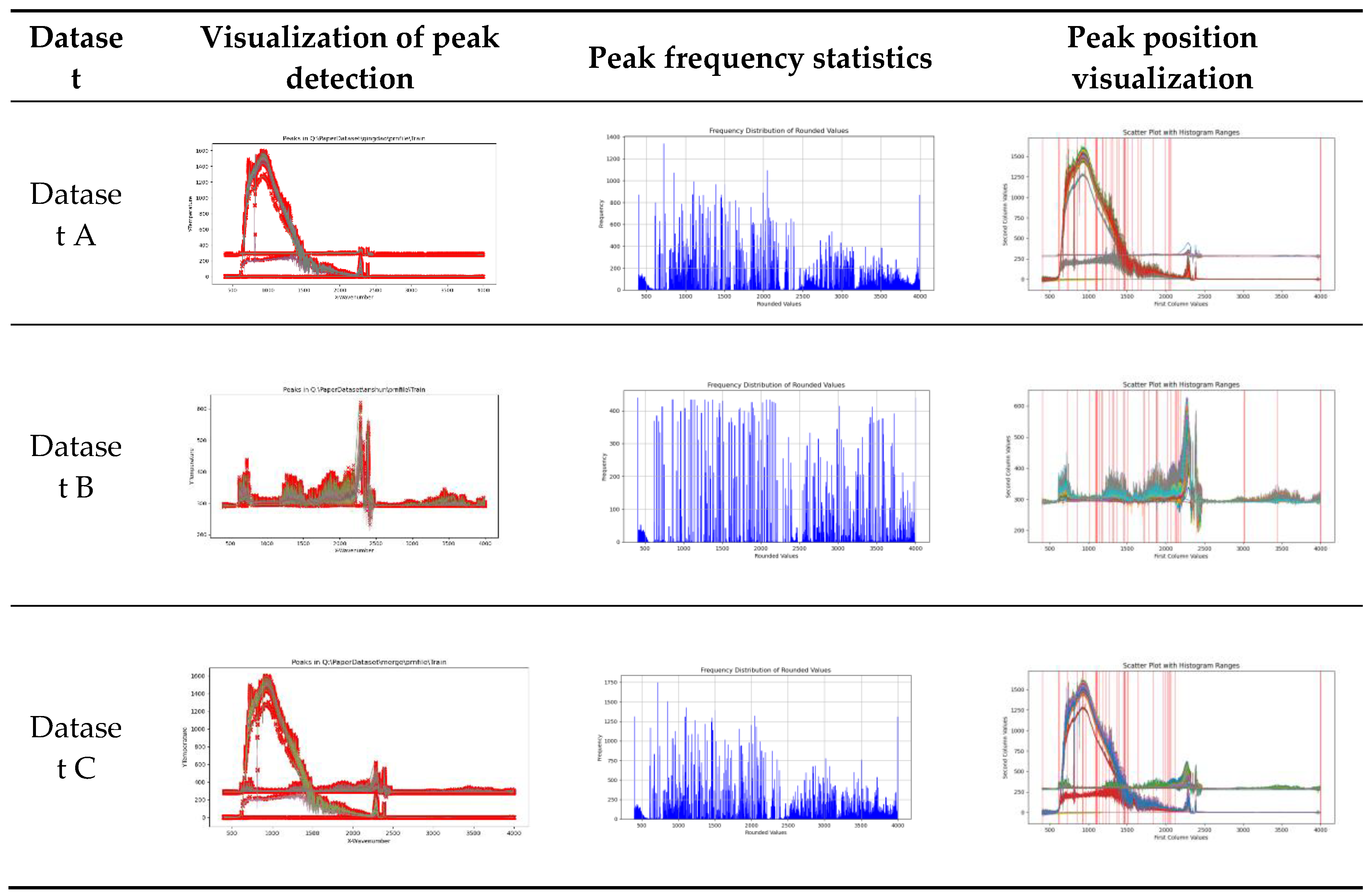
(1) Effectiveness of peak features: The effectiveness of peak features for algorithm improvement can be verified by the effect of combining peak features with traditional classifiers for data classification. We seek peaks on three data sets and obtain experimental results as presented in Figure 9:

Among them, the three graphs on the left with red points indicate the wavelet algorithm's extracted peak points, the three graphs in the middle show the data set's frequency of these peak points, and the three graphs on the right with red lines indicate the location of the points with higher frequency in the spectral data set. According to the intersection of the high frequency wavenumber positions of data set A and data set B, we get 13 peak wavenumber positions, which are 403,720,853, 1091, 1107, 1226, 1462, 1502, 2042 and 3998, respectively. At the same time, we calculate the data of the 13 peak positions of each data, and combine the two classifier methods SVM and XGBoost, which are generally and well performed in the above experiment, and get the classification results as shown in Table 16:

Combined with the experimental results, the peak data we extracted is effective, compared with the CO₂ feature vector and classifier algorithm, all the performance results are improved. The experimental results show that the peak seeking algorithm is effective for classification tasks.

(2)Effectiveness of AM:The experimental results of three data sets with CNN with the same parameters of Table 7 are shown in the Table 17:

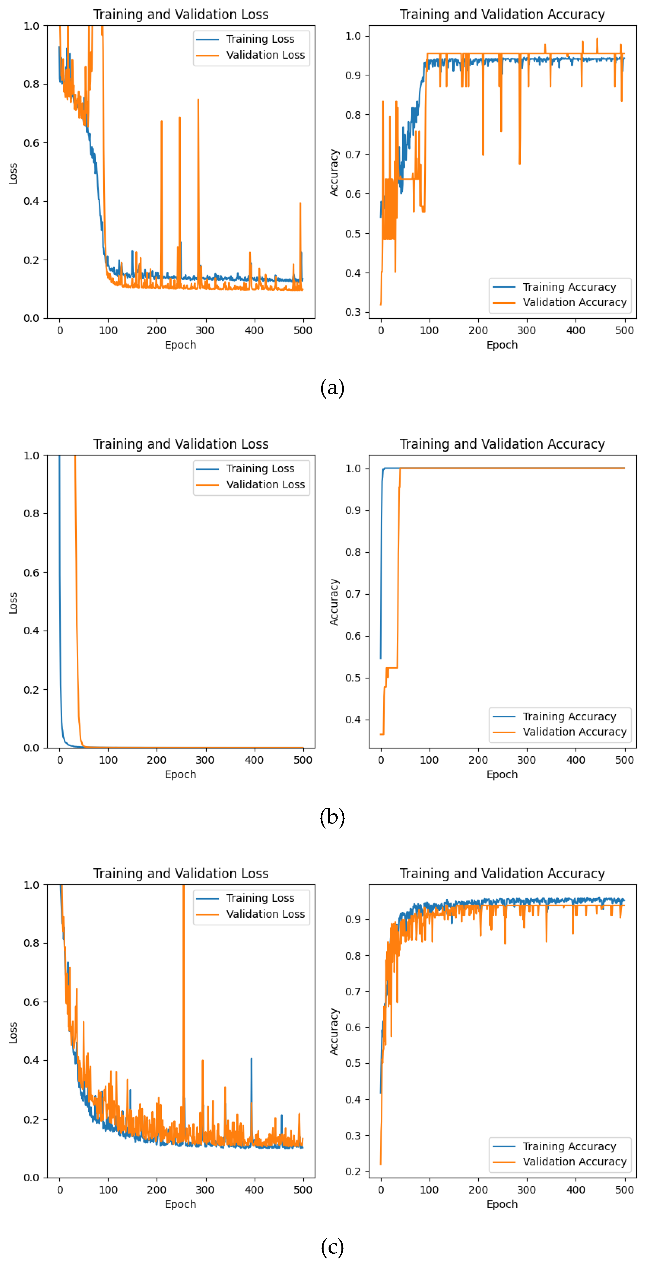
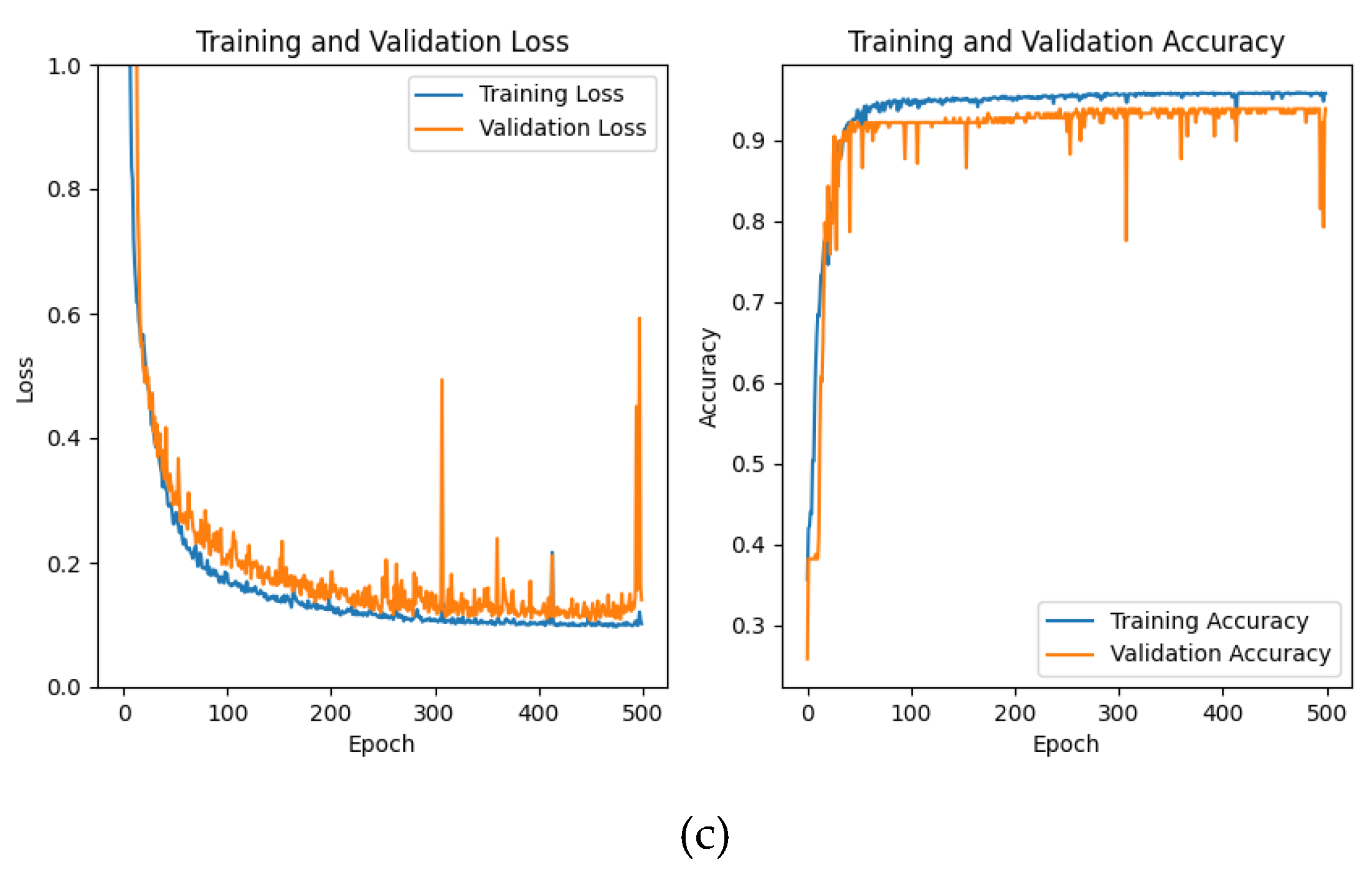
Figure 10. CNN network training and validation loss function and accuarcy change curve: the blue curve represents the training set, the orange curve represents the validation set, (a) is the experimental result of dataset a, (b) is the experimental result of dataset B, and (c) is the experimental result of dataset C

The CNN structure designed in this paper performs well on all three data sets, and the accuracy is more than 90%. There are a few misclassifications above Dataset A and Dataset C. Compared with CWT-AM-CNN, only using backbone network for classification will occur Loss shock, and compared with CWT-AM-CNN, its convergence speed is slightly lower and the accuracy is also slightly lower.

(3) Comparison of network design:

①Effectiveness of BN layer design: Remove the BN layer using the same parameters in Table 7 to get the experimental results such as Table 18:

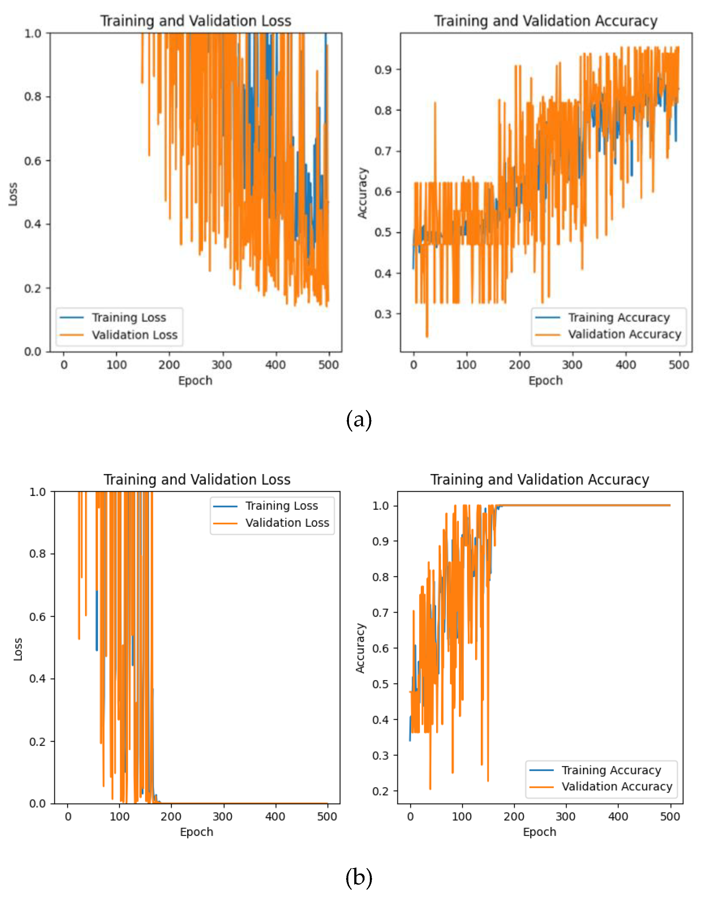
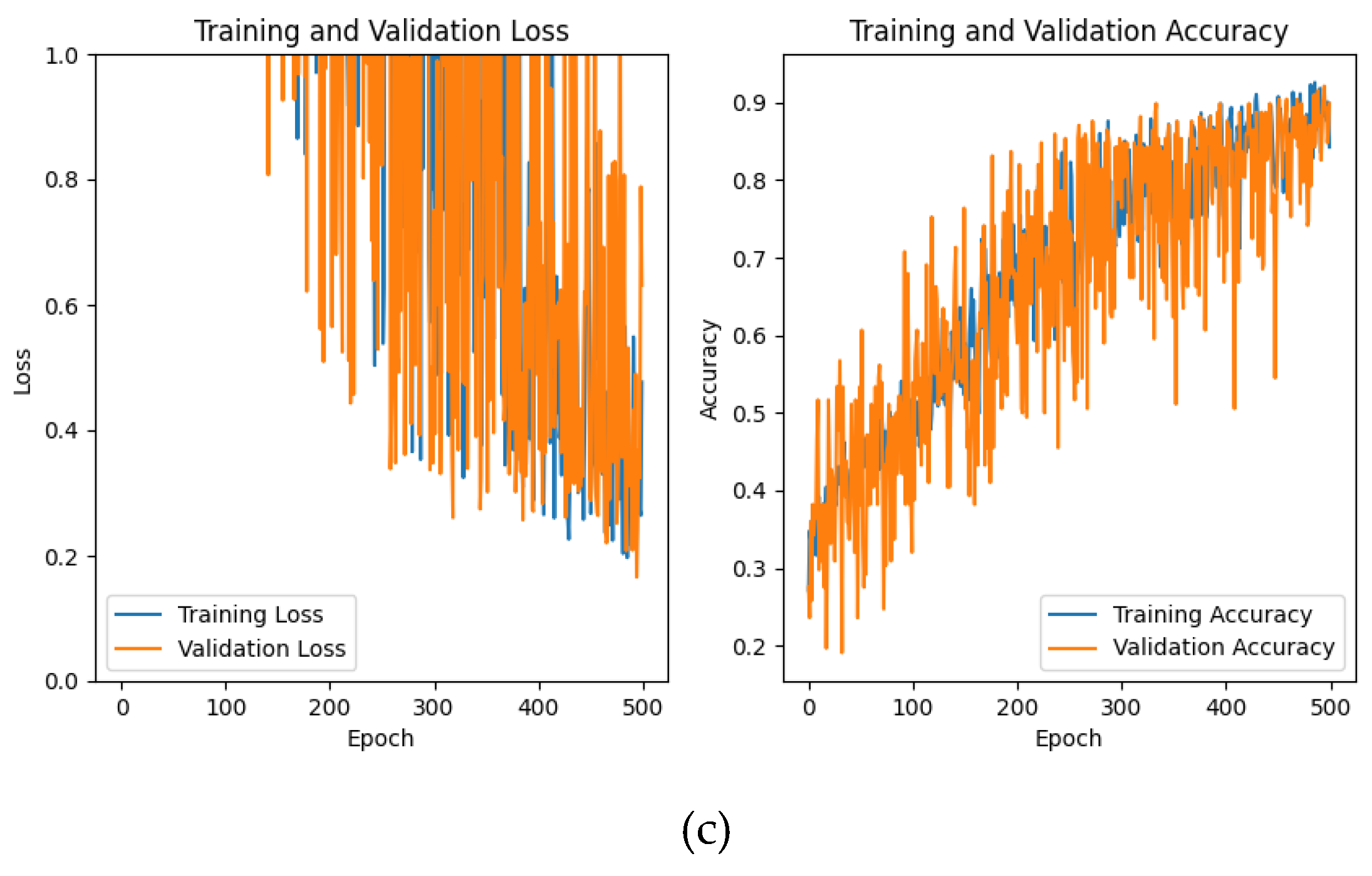
Figure 11. Loss function and accuracy change curve of CNN (without BN layer) network training and validation: the blue curve represents the training set, the orange curve represents the validation set, (a) is the experimental result of dataset a, (b) is the experimental result of dataset B, and (c) is the experimental result of dataset C

Only using the CNN network without BN layer network structure in this paper also has a good classification accuracy, while the Loss curve and the accuracy change curve have a great shock in the process of training, which shows that the model is too sensitive to the training data, and the model is unstable, which will affect the results of our classification experiments.

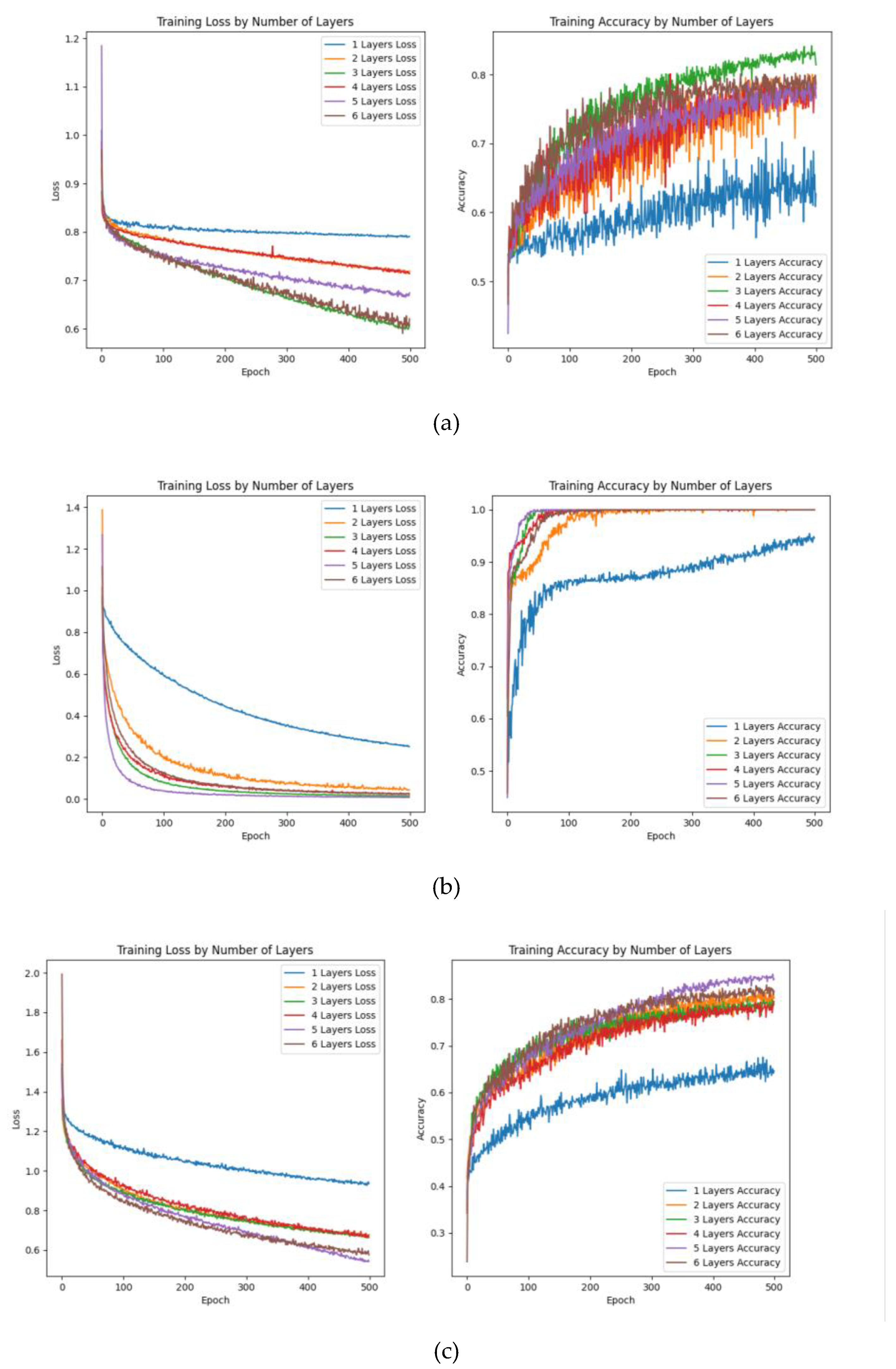
②Network depth: In deep learning algorithms, network depth carries out a decisive role in network expression. The deeper the depth, the better the network expression, because network depth determines the quality of features from aspects such as invariance and abstraction. Therefore, we conduct an experimental comparison of networks with different layer structures. Each layer uses a feature extraction block, and uses the same loss function, optimizer, and learning rate to get Table 19:

In general, CNN with three layer feature extraction blocks as the structure has excellent results in training time and accuracy, so we adopt it as the structure of our backbone network.

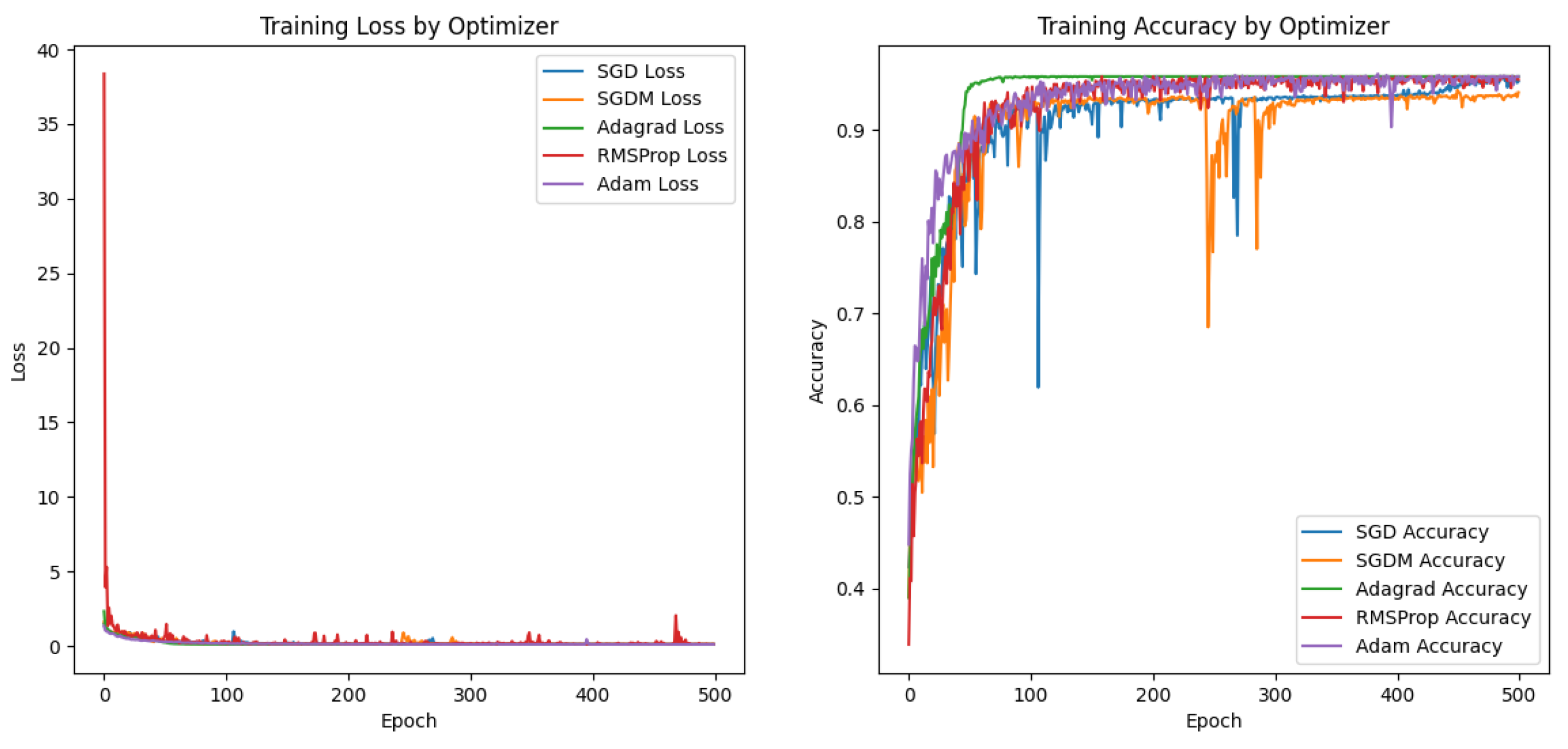
③Optimizer selection:The five optimizers are essentially divided into two categories, SGD, SGDM and Adagrad, RMSProp, Adam. The most frequently used ones are SGDM and Adam. We test the backbone network with different optimizers on our data set and get table Table 20:

By comparing the outcomes, we can observe that the Adagrad and Adam tables on our network and dataset are now quite good. The Adam algorithm has better adaptability and convergence effect, so this paper manipulates Adam as the optimizer.

④Selection of learning rate: In the training of the data set, the loss curve shows a situation of concussion. Given this scenario, we examine our data set using various learning rates and descent in increments of 10⁻¹ from 0.001 to generate Table 21:

The learning rate affects the classification effect of the network to a great extent. From the prediction accuracy, running time and loss function training effect, the comprehensive effect of the learning rate at 0.00001 is the best.

(4) Running time: Compared with the traditional classifier method, the deep learning method needs to expend more time on the model training. However, the advantage of the deep learning method is in the trained model. We compare the prediction time of the proposed algorithm and each method on three data sets and obtain the following expression, as shown in Table 22:

Table 22 shows that in terms of running time, most of the traditional classifier methods and AE methods have high running efficiency. The CWT-AM-CNN method and the same structure CNN also have higher running efficiency in prediction. The running efficiency of LSTM method is a little slower, and the running efficiency of RNN is the worst. The network's drawback compared to the classifier is the extended training time, but it offers increased running efficiency post-training.

5. Conclusions

In order to classify aero-engines, the infrared spectrum of hot jets of six different types aero-engines in various states are measured using a telemetry FT-IR spectrometer, and three data sets are created in this article. This study presents the design of a CNN based on peak seeking attention mechanism, named after CWT-AM-CNN. The medium wave band peak value is determined by CWT, the high frequency wave number position is tallied, and the peak data is recovered. Attention mechanism is adopted for the peak data, and the feature graph of feature extraction network is weighted by attention mechanism. The training set, validation set and prediction set were randomly sampled according to the ratio of 8:1:1; The CWT-AM-CNN was trained, verified and predicted, and the ablation experiment was conducted for experimental comparison. The accuracy, precision, recall, confusion matrix and F1-score are used to evaluate the classification results. the accuracy of the prediction on three data sets is as high as 97%. Comparing the experimental findings with the classifier algorithm based on feature vector and the current popular network approaches, AE, RNN, and LSTM, reveals that CWT-AM-CNN is effective, practical, and can achieve excellent classification accuracy. It is proposed that CWT-AM-CNN has higher accuracy and better stability for three different data sets, and can complete the task of infrared spectral classification of aero-engine hot jets.

Author Contributions

Formal analysis, Y.L.; investigation, S.D. and Z.L.; software, Z.K. and X.L.; validation, W.H. and Z.L. All authors have read and agreed to the published version of the manuscript.

Funding

This research was funded by National Natural Science Foundation of China, grant number 62005320.

Data Availability Statement

The data presented in this study are available upon request from the corresponding author.

Conflicts of Interest

The authors declare no conflicts of interest.

References

Manijeh,Razeghi,Binh-Minh,et al.Advances in mid-infrared detection and imaging: a key issues review.Reports on Progress in Physics, 2014.
Chikkaraddy R, Arul R, Jakob L A,et al.Single-molecule mid-IR detection through vibrationally-assisted luminescence. 2022.
Knez D, Toulson B W, Chen A,et al.Spectral imaging at high definition and high speed in the mid-infrared.Science advances, 2022(46).
Zhang J, Gong Y.Automated identification of infrared spectra of hazardous clouds by passive FTIR remote sensing//Multispectral & Hyperspectral Image Acquisition & Processing.International Society for Optics and Photonics, 2001.
Roh S B, Oh S K. Identification of Plastic Wastes by Using Fuzzy Radial Basis Function Neural Networks Classifier with Conditional Fuzzy C-Means Clustering. Journal of Electrical Engineering & Technology, 2016, 11, 103–116.
Vinayak V, Gautam S, Namdeo V,et al.Fast Fourier infrared spectroscopy to characterize the biochemical composition in diatoms. (Accepted, Sept 2018, Vol 3 no-4).Journal of Biosciences, 2018, 3.
Han X, Li X, Gao M, et al. Emissions of Airport Monitoring with Solar Occultation Flux-Fourier Transform Infrared Spectrometer. Journal of Spectroscopy, 2018, 2018, 1–10.
Cięszczyk, S. Passive open-path FTIR measurements and spectral interpretations for in situ gas monitoring and process diagnostics. Acta Physica Polonica A, 2014, 126, 673–678. [Google Scholar] [CrossRef]
Schütze C, Lau S, Reiche N, et al. Ground-based remote sensing with open-path Fourier-transform infrared (OP-FTIR) spectroscopy for large-scale monitoring of greenhouse gases. Energy Procedia, 2013, 37, 4276–4282.
YANG L, TAO Z. Aircraft image recognition in airport flight area based on deep transfer learning//International Conference on Smart Transportation and City Engineering 2021, Chongqing, China. 2021.
Shen, H. , Huo, K. , Qiao, X., & Li, C. Aircraft target type recognition technology based on deep learning and structure feature matching. Intell. Fuzzy Syst. 2023, 45, 5685–5696. [Google Scholar]
LI X, LI Z, QIU H, et al. An overview of hyperspectral image feature extraction, classification methods and the methods based on small samples. Applied Spectroscopy Reviews, 2021: 1-34.
Vaswani, A. , Shazeer, N.M., Parmar, N., Uszkoreit, J., Jones, L., Gomez, A.N., Kaiser, L., & Polosukhin, I. (2017). Attention is All you Need. Neural Information Processing Systems.
AUDEBERT N, LE SAUX B, LEFEVRE S. Deep Learning for Classification of Hyperspectral Data: A Comparative Review. IEEE Geoscience and Remote Sensing Magazine, 2019, 159-173.
RASTI B, HONG D, HANG R, et al. Feature Extraction for Hyperspectral Imagery: The Evolution From Shallow to Deep: Overview and Toolbox. IEEE Geoscience and Remote Sensing Magazine, 2020, 60-88.
Lu, W.; Wang, X.; Sun, L.; Zheng, Y. Spectral–Spatial Feature Extraction for Hyperspectral Image Classification Using Enhanced Transformer with Large-Kernel Attention. Remote Sens. 2024, 16, 67. [Google Scholar] [CrossRef]
CHEN Y, LIN Z, ZHAO X, et al. Deep Learning-Based Classification of Hyperspectral Data. IEEE Journal of Selected Topics in Applied Earth Observations and Remote Sensing, 2014, 2094-2107.
KEMKER R, KANAN C. Self-Taught Feature Learning for Hyperspectral Image Classification. IEEE Transactions on Geoscience and Remote Sensing, 2017, 2693-2705.
DING Y, ZHAO X, ZHANG Z, et al. Graph Sample and Aggregate-Attention Network for Hyperspectral Image Classification. IEEE Geoscience and Remote Sensing Letters, 2022: 1-5.
LI Z, ZHAO B, WANG W. An Efficient Spectral Feature Extraction Framework for Hyperspectral Images. Remote Sensing, 2020, 3967.
Ashraf, M.; Zhou, X.; Vivone, G.; Chen, L.; Chen, R.; Majdard, R.S. Spatial-Spectral BERT for Hyperspectral Image Classification. Remote Sens. 2024, 16, 539. [Google Scholar] [CrossRef]
HAMOUDA M, ETTABAA K S, BOUHLEL M S. Smart feature extraction and classification of hyperspectral images based on convolutional neural networks. IET Image Processing, 2020, 14(10): 1999-2005.
LECUN Y, BOTTOU L, BENGIO Y, et al. Gradient-based learning applied to document recognition. Proceedings of the IEEE, 1998, 2278-2324.
KRIZHEVSKY A, SUTSKEVER I, HINTON G E. ImageNet Classification with Deep Convolutional Neural Networks. Communications of the ACM, 2017: 84-90.
SIMONYAN K, ZISSERMAN A. Very Deep Convolutional Networks for Large-Scale Image Recognition. International Conference on Learning Representations,International Conference on Learning Representations, 2015.
SZEGEDY C, WEI LIU, YANGQING JIA, et al. Going deeper with convolutions//2015 IEEE Conference on Computer Vision and Pattern Recognition (CVPR), Boston, MA, USA. 2015.
HE K, ZHANG X, REN S, et al. Deep Residual Learning for Image Recognition//2016 IEEE Conference on Computer Vision and Pattern Recognition (CVPR), Las Vegas, NV, USA. 2016.
IOFFE S, SZEGEDY C. Batch Normalization: Accelerating Deep Network Training by Reducing Internal Covariate Shift. arXiv: Learning,arXiv: Learning, 2015.
Doubenskaia, M.; Pavlov, M.; Grigoriev, S.; Smurov, I. Definition of brightness temperature and restoration of true temperature in laser cladding using infrared camera. Surf. Coat. Technol. 2013, 220, 244–247. [Google Scholar] [CrossRef]
Homan, D.C.; Cohen, M.H.; Hovatta, T.; Kellermann, K.I.; Kovalev, Y.Y.; Lister, M.L.; Popkov, A.V.; Pushkarev, A.B.; Ros, E.; Savolainen, T. MOJAVE. XIX. Brightness Temperatures and Intrinsic Properties of Blazar Jets. Astrophys. J. 2021, 923, 67. [Google Scholar]
HU J, SHEN L, ALBANIE S, et al. Squeeze-and-Excitation Networks. IEEE Transactions on Pattern Analysis and Machine Intelligence, 2020: 2011-2023.
WOO S, PARK J, LEE J Y, et al. CBAM: Convolutional Block Attention Module//Computer Vision – ECCV 2018,Lecture Notes in Computer Science. 2018: 3-19.
WANG Q, WU B, ZHU P, et al. ECA-Net: Efficient Channel Attention for Deep Convolutional Neural Networks//2020 IEEE/CVF Conference on Computer Vision and Pattern Recognition (CVPR), Seattle, WA, USA. 2020.
LI X, HU X, YANG J. Spatial Group-wise Enhance: Improving Semantic Feature Learning in Convolutional Networks. Cornell University - arXiv,Cornell University - arXiv, 2019.
KINGMA DiederikP, BA J. Adam: A Method for Stochastic Optimization. arXiv: Learning,arXiv: Learning, 2014.

Figure 1. CWT-AM-CNN classification network of aero-engine hot jet infrared spectrum.

Figure 2. Feature extraction block.

Figure 3. Composition diagram of attention mechanism module based on peak seeking: (a) represents peak seeking algorithm block, (b) represents attention mechanism block.

Figure 4. Attention mechanism operation diagram.

Figure 5. Site layout of outfield measurement experiment for infrared spectrum of aeroengine hot jet.

Figure 6. Experimental measurement of the BTSs of aero- engines’ hot jet.

Figure 7. CWT-AM-CNN network training and validation loss function and accuarcy change curve: the blue curve represents the training set, the orange curve represents the validation set, (a) is the experimental result of dataset a, (b) is the experimental result of dataset B, and (c) is the experimental result of dataset C

Figure 8. Four characteristic peak positions in the infrared spectrum of aero-engine hot jet.

Figure 9. Experimental results of CWT peak detection and high frequency peak statistics.

Figure 12. Training and validation of CNN network with different layers loss function and accuarcy change curve: the blue curve represents the one layer structure, the orange curve represents the two layer structure, the green represents the three layer structure, the red represents the four layer structure, the purple represents the five layer structure, and the brown represents the six layer structure, (a) is the experimental result of dataset A, (b) is the experimental result of dataset B, and (c) is the experimental result of dataset C

Figure 13. Network training and validation of the different optimizers on dataset C loss function and accuracy change curve: blue is SGD, orange is SGDM, green is Adagrad, red is RMSProp, and purple is Adam.

Figure 14. Network training and validation of Adam optimizer with different learning rates on dataset C loss function and accuracy change curve: blue is the learning rate of 0.01, orange is the learning rate of 0.001, green is the learning rate of 0.0001, red is the learning rate of 0.00001, and purple is the learning rate of 0.000001.

Table 1. Parameters of the FT-IR spectrometers used for the experiment.

Name	Measurement Pattern	Spectral Resolution (cm⁻¹)	Spectral Measurement Range (µm)	Full Field of View Angle
EM27	Active/Passive	Active: 0.5/1 Passive: 0.5/1/4	2.5~12	30 mrad (no telescope) (1.7°)
Telemetry Fourier Transform Infrared Spectrometer	Passive	1	2.5~12	1.5°

Table 2. Table of experimental aero-engines and environmental factors.

Aero-Engine Serial Number	Environmental Temperature	Environmental Humidity	Detection Distance
Turbofan engine 1	19℃	58.5%Rh	5m
Turbofan engine 2	16℃	67%Rh	5m
Turbojet engine	14℃	40%Rh	5m
Turbojet UAV	30℃	43.5%Rh	11.8m
Turbojet UAV with propeller at tail	20℃	71.5%Rh	5m
Turbojet manned aircraft	19℃	73.5%Rh	10m

Table 3. Dataset A information table.

Label	Type	Number of data pieces	Number of error data	Full band data volume	Medium wave range data volume
1	Turbofan engine 1	792	17	16384(1cm⁻¹)/32768(0.5cm⁻¹)	7464/14928
2	Turbofan engine 2	258	2	16384(1cm⁻¹)/32768(0.5cm⁻¹)	7464/14928
3	Turbojet engine	384	4	16384(1cm⁻¹)/32768(0.5cm⁻¹)	7464/14928

Table 4. Dataset B information table.

Label	Type	Number of data pieces	Number of error data	Full band data volume	Medium wave range data volume
1	Turbojet UAV	193	0	16384	7464
2	Turbojet UAV with propeller at tail	48	0	16384	7464
3	Turbojet manned aircraft	202	3	16384	7464

Table 5. Dataset C information table.

Label	Type	Number of data pieces	Number of error data	Full band data volume	Medium wave range data volume
1	Turbojet UAV	193	0	16384	7464
2	Turbojet UAV with propeller at tail	48	0	16384	7464
3	Turbojet manned aircraft	202	3	16384	7464
4	Turbofan engine 1	792	17	16384	7464
5	Turbofan engine 2	258	2	16384	7464
6	Turbojet engine	384	4	16384	7464

Where, Dataset C is the combination of Dataset A and Dataset B.

Table 6. Confusion matrix.

		Forecast results
		Positive samples	Negative samples
Real results	Positive samples	TP	TN
Real results	Negative samples	FP	FN

Table 7. Parameter table of CWT-AM-CNN model.

Methods	Parameter Settings
CWT-AM-CNN	Conv1D(32, 3) ,Conv1D(64, 3), Conv1D(128, 3)，activation='relu'
	BatchNormalization()
	MaxPooling1D(2)(x)
	Dense(128, activation='relu')，activation='softmax'
	Optimizers=Adam ，lr=0.00001
	loss='sparse_categorical_crossentropy',metrics=['accuracy'])
	epochs=500

Table 8. Results of CWT-AM-CNN classification experiments.

	Accuracy	Precision score	Recall	Confusion matrix	F1-score
Datasets	Accuracy	Precision score	Recall	Confusion matrix	F1-score
DatasetA	97.44%	94.08%	85.11%	[11 8 0] [ 0 77 0] [ 1 0 38]	88.24%
DatasetB	100.00%	100.00%	100.00%	[19 0 0] [ 0 8 0] [ 0 0 17]	100.00%
DatasetC	100%	98.72%	94.70%	[17 0 0 0 0 0] [ 0 7 0 0 0 0] [ 0 0 16 0 0 0] [ 0 0 0 84 0 0] [ 0 0 0 7 15 0] [ 0 0 0 0 0 33]	96.18%

Table 9. Value range of characteristic peak threshold.

Characteristic Peak Type	Emission Peak (cm⁻¹)			Absorption Peak (cm⁻¹)
Peak standard features	2350	2390	720	667
Characteristic peak range values	2350.5-2348	2377-2392	722-718	666.7-670.5

Table 10. Parameter table of classifier method based on feature vector.

Methods	Parameter Settings
SVM	decision_function_shape = ‘ovr’, kernel = ‘rbf’
XGBoost	objective = ‘multi:softmax’, num_classes = num_classes
CatBoost	loss_function = ‘MultiClass’
Adaboost	n_estimators = 200
Random Forest	n_estimators = 300
LightGBM	objective’: ‘multiclass’, ‘num_class’: num_classes
Neural Network	hidden_layer_sizes = (100), activation = ‘relu’, solver = ‘adam’, max_iter = 200

Table 11. Experimental results of classifier method based on feature vector on Dataset A.

	Accuracy	Precision score	Recall	Confusion matrix	F1-score
Classification methods	Accuracy	Precision score	Recall	Confusion matrix	F1-score
Feature vector+SVM	57.04%	33.33%	19.01%	[ 0 0 0] [19 77 39] [ 0 0 0]	24.21%
Feature vector+XGBoost	96.30%	96.09%	94.36%	[18 3 0] [ 1 74 1] [ 0 0 38]	95.14%
Feature vector+CatBoost	97.04%	96.53%	95.80%	[18 2 0] [ 1 75 1] [ 0 0 38]	96.14%
Feature vector+AdaBoost	74.81%	74.29%	71.93%	[11 25 0] [ 8 52 1] [ 0 0 38]	71.35%
Feature vector+Random Forest	97.04%	96.53%	95.80%	[18 2 0] [ 1 75 1] [ 0 0 38]	96.14%
Feature vector+LightGBM	96.30%	96.09%	94.36%	[18 3 0] [ 1 74 1] [ 0 0 38]	95.14%
Feature vector+Neural Networks	86.67%	68.42%	92.64%	[ 1 0 0] [16 77 0] [ 2 0 39]	66.03%

Table 12. Experimental results of classifier method based on feature vector on Dataset B.

	Accuracy	Precision score	Recall	Confusion matrix	F1-score
Classification methods	Accuracy	Precision score	Recall	Confusion matrix	F1-score
Feature vector+SVM	86.36%	88.24%	92.00%	[19 0 6] [ 0 8 0] [ 0 0 11]	88.31%
Feature vector+XGBoost	84.09%	86.48%	88.89%	[18 0 6] [ 0 8 0] [ 1 0 11]	86.53%
Feature vector+CatBoost	86.36%	88.24%	92.00%	[19 0 6] [ 0 8 0] [ 0 0 11]	88.31%
Feature vector+AdaBoost	77.27%	80.60%	85.19%	[18 0 9] [ 0 8 0] [ 1 0 8]	79.93%
Feature vector+Random Forest	86.36%	88.24%	92.00%	[19 0 6] [ 0 8 0] [ 0 0 11]	88.31%
Feature vector+LightGBM	84.09%	86.48%	88.89%	[18 0 6] [ 0 8 0] [ 1 0 11]	86.53%
Feature vector+Neural Networks	88.64%	90.20%	93.06%	[19 0 5] [ 0 8 0] [ 0 0 12]	90.38%

Table 13. Table 13. Experimental results of classifier method based on feature vector on Dataset C.

	Accuracy	Precision score	Recall	Confusion matrix	F1-score
Classification methods	Accuracy	Precision score	Recall	Confusion matrix	F1-score
Feature vector+SVM	59.78%	44.15%	47.67%	[ 8 0 3 0 0 0] [ 0 3 0 0 0 0] [ 9 1 12 0 0 0] [ 0 3 1 84 22 33] [ 0 0 0 0 0 0] [ 0 0 0 0 0 0]	42.38%
Feature vector+XGBoost	94.97%	92.44%	93.59%	[15 0 3 0 0 0] [ 0 7 0 0 0 0] [ 2 0 13 0 0 0] [ 0 0 0 83 3 0] [ 0 0 0 1 19 0] [ 0 0 0 0 0 33]	92.95%
Feature vector+CatBoost	94.41%	90.35%	93.52%	[15 0 2 0 0 0] [ 0 6 0 0 0 0] [ 2 0 14 0 0 0] [ 0 0 0 83 4 0] [ 0 1 0 1 18 0] [ 0 0 0 0 0 33]	91.81%
Feature vector+AdaBoost	79.89%	63.66%	71.49%	[17 5 6 0 0 0] [ 0 2 0 0 0 0] [ 0 0 10 0 0 0] [ 0 0 0 84 18 3] [ 0 0 0 0 0 0] [ 0 0 0 0 4 30]	62.56%
Feature vector+Random Forest	94.41%	91.40%	92.70%	[15 0 4 0 0 0] [ 0 7 0 0 0 0] [ 2 0 12 0 0 0] [ 0 0 0 83 3 0] [ 0 0 0 1 19 0] [ 0 0 0 0 0 33]	91.91%
Feature vector+LightGBM	94.41%	90.68%	92.40%	[14 0 2 0 0 0] [ 0 6 0 0 0 0] [ 3 0 14 0 0 0] [ 0 0 0 82 2 0] [ 0 1 0 2 20 0] [ 0 0 0 0 0 33]	91.42%
Feature vector+Neural Networks	84.92%	76.79%	76.57%	[17 0 2 0 0 0] [ 0 6 0 0 0 0] [ 0 0 12 0 0 0] [ 0 0 2 84 18 0] [ 0 1 0 0 0 0] [ 0 0 0 0 4 33]	76.02%

Table 14. Parameters of common deep learning networks.

Methods	Parameter Settings
AE	Dense(encoding_dim,activation="relu") Dense(input_dim, activation="sigmoid") Dense(num_classes, activation="softmax") epochs=500, optimizer= Adam(lr=0.00001),loss='sparse_categorical_crossentropy', metrics=['accuracy']
RNN	SimpleRNN(4, return_sequences=True) BatchNormalization() Dense(4, activation='relu') Dense(num_classes, activation='softmax') epochs=500, optimizer= Adam(lr=0.00001),loss='sparse_categorical_crossentropy', metrics=['accuracy']
LSTM	LSTM(8, return_sequences=True),BatchNormalization() LSTM(8),BatchNormalization() Dense(8, activation='relu')) Dense(num_classes, activation='softmax') epochs=500, optimizer= Adam(lr=0.00001),loss='sparse_categorical_crossentropy', metrics=['accuracy']

Table 15. Results of common deep learning network classification experiments.

Methods	Dataset	Accuracy	Precision score	Recall	Confusion matrix	F1-score
AE	A	58.52%	52.63%	36.84%	[ 2 17 0] [ 0 77 0] [ 0 39 0]	30.79%
	B	38.64%	12.88%	33.33%	[ 0 0 19] [ 0 0 8] [ 0 0 17]	18.58%
	C	46.93%	7.82%	16.67%	[ 0 0 0 17 0 0] [ 0 0 0 7 0 0] [ 0 0 0 16 0 0] [ 0 0 0 84 0 0] [ 0 0 0 22 0 0] [ 0 0 0 33 0 0]	10.65%
RNN	A	38.64%	12.88%	33.33%	[ 0 0 19] [ 0 0 8] [ 0 0 17]	18.58%
	B	57.03%	19.01%	33.33%	[ 0 19 0] [ 0 77 0] [ 0 39 0]	24.21%
	C	46.92%	7.80%	16.66%	[ 0 0 0 17 0 0] [ 0 0 0 7 0 0] [ 0 0 0 16 0 0] [ 0 0 0 84 0 0] [ 0 0 0 22 0 0] [ 0 0 0 33 0 0]	10.64%
LSTM	A	38.63%	12.88%	33.33%	[ 0 0 19] [ 0 0 8] [ 0 0 17]	18.58%
	B	57.03%	19.01%	33.33%	[ 0 19 0] [ 0 77 0] [ 0 39 0]	24.21%
	C	62.57%	48.72%	41.91%	[ 4 0 13 0 0 0] [ 0 0 7 0 0 0] [ 0 0 16 0 0 0] [ 0 0 0 82 0 2] [ 0 0 0 22 0 0] [ 0 0 0 23 0 10]	36.97%

Table 16. Experimental results of peak seeking classifier classification.

SVM	Accuracy	Precision	Recall	Confusion Matrix	F1-score	Running time
Dataset A	59.26%	51.08%	42.27%	[ 0 0 0] [10 41 0] [ 9 36 39]	42.49%	0.131497
Dataset B	100.00%	100.00%	100.00%	[19 0 0] [ 0 8 0] [ 0 0 17]	100.00%	0.008979
Dataset C	56.98%	46.13%	44.43%	[ 4 0 0 0 0 0] [ 0 0 0 0 0 0] [13 7 15 0 0 0] [ 0 0 0 50 11 0] [ 0 0 0 0 0 0] [ 0 0 1 34 11 33]	37.47%	0.24201
XGBoost	Accuracy	Precision	Recall	Confusion Matrix	F1-score	Running time
Dataset A	100.00%	100.00%	100.00%	[19 0 0] [ 0 8 0] [ 0 0 17]	100.00%	0.135857
Dataset B	99.26%	99.15%	99.57%	[19 0 0] [ 0 77 1] [ 0 0 38]	99.35%	0.204039
Dataset C	98.88%	95.24%	98.15%	[17 0 0 0 0 0] [ 0 5 0 0 0 0] [ 0 2 16 0 0 0] [ 0 0 0 84 0 0] [ 0 0 0 0 22 0] [ 0 0 0 0 0 33]	96.24%	0.34023

Table 17. Results of CNN classification experiment.

	Accuracy	Precision score	Recall	Confusion matrix	F1-score
Datasets	Accuracy	Precision score	Recall	Confusion matrix	F1-score
Dataset A	94.07%	96.86%	85.96%	[11 8 0] [ 0 77 0] [ 0 0 39]	89.47%
Dataset B	100%	100%	100%	[19 0 0] [ 0 8 0] [ 0 0 17]	100%
Dataset C	96.09%	98.72%	94.70%	[17 0 0 0 0 0] [ 0 7 0 0 0 0] [ 0 0 16 0 0 0] [ 0 0 0 84 0 0] [ 0 0 0 7 15 0] [ 0 0 0 0 0 33]	96.18%

Table 18. Results of CNN (without BN layer) classification experiment.

	Accuracy	Precision score	Recall	Confusion matrix	F1-score
Datasets	Accuracy	Precision score	Recall	Confusion matrix	F1-score
Dataset A	92.59%	91.70%	84.68%	[11 8 0] [ 1 76 0] [ 1 0 38]	87.29%
Dataset B	100%	100%	100%	[19 0 0] [ 0 8 0] [ 0 0 17]	100%
Dataset C	92.18%	94.11%	89.94%	[17 0 0 0 0 0] [ 0 7 0 0 0 0] [ 4 0 12 0 0 0] [ 0 0 0 81 0 3] [ 0 0 0 7 15 0] [ 0 0 0 0 0 33]	91.02%

Table 19. Results of network depth comparison.

Dataset	Number of layers Evaluation	1	2	3	4	5	6
Dataset A	Accuracy	63%	66%	83%	81%	79%	82%
	Training Time /s	315.83	939.22	1332.54	1527.18	1735.24	2032.12
	Evaluation Time/s	0.14	0.18	0.22	0.33	0.35	0.32
Dataset B	Accuracy	93%	100%	100%	100%	100%	100%
	Training Time /s	81.90	148.38	258.92	347.15	408.00	431.55
	Evaluation Time/s	0.12	0.13	0.18	0.25	0.22	0.25
Dataset C	Accuracy	63%	74%	77%	73%	78%	82%
	Training Time /s	421.56	1088.86	1522.65	2014.09	2411.60	2850.66
	Evaluation Time/s	0.16	0.15	0.21	0.23	0.30	0.36

Table 20. Results of different optimizer experiments.

Optimizers	Prediction accuracy	Training time/s	Prediction time/s
SGD	93%	1663.36	0.25
SGDM	93%	2074.59	0.23
Adagrad	94%	2133.88	0.24
RMSProp	89%	2194.60	0.27
Adam	94%	2165.09	0.24

Table 21. Table of experimental results of optimizer Adam at different learning rates.

Learning rate	Prediction accuracy	Training time/s	Prediction time/s
0.01	0.47	878.21	0.26
0.001	0.75	1215.80	0.20
0.0001	0.42	1246.89	0.21
0.00001	0.95	1241.00	0.22
0.000001	0.95	1221.39	0.21

Table 22. Comparison table of classified prediction running time.

Method	Running time /s
Method	Dataset A	Dataset B	Dataset C
CNN	5	4	6
CNN-BN	5	4	5
CWT-AM-CNN	6	5	6
RNN	980	243	1151
LSTM	14	4	17
AE	0.025	0.025	0.026
Feature vector+SVM	0.08	0.01	0.12
Feature vector+XGBoost	0.17	0.24	0.30
Feature vector+CatBoost	3.09	2.61	4.74
Feature vector+AdaBoost	0.30	0.26	0.39
Feature vector+Random Forest	0.48	0.44	0.56
Feature vector+LightGBM	0.20	0.17	0.44
Feature vector+Neural Networks	0.29	0.31	0.85

Disclaimer/Publisher’s Note: The statements, opinions and data contained in all publications are solely those of the individual author(s) and contributor(s) and not of MDPI and/or the editor(s). MDPI and/or the editor(s) disclaim responsibility for any injury to people or property resulting from any ideas, methods, instructions or products referred to in the content.

© 2024 by the authors. Licensee MDPI, Basel, Switzerland. This article is an open access article distributed under the terms and conditions of the Creative Commons Attribution (CC BY) license (https://creativecommons.org/licenses/by/4.0/).

Copyright: This open access article is published under a Creative Commons CC BY 4.0 license, which permit the free download, distribution, and reuse, provided that the author and preprint are cited in any reuse.

MDPI Initiatives

Important Links

Choose an area of interest and we will send you notifications of new preprints at your preferred frequency.

Disclaimer