Revisiting Fold-Change Calculation: Preference for Median or Geometric Mean over Arithmetic Mean-Based Methods

Preprint

Brief Report

Revisiting Fold-Change Calculation: Preference for Median or Geometric Mean over Arithmetic Mean-Based Methods

Altmetrics

Downloads

102

Views

Comments

This version is not peer-reviewed

Submitted:

19 June 2024

Posted:

20 June 2024

You are already at the latest version

Alerts

Abstract

Background: Fold change is widely used in biomedical research to quantify the magnitude of group differences in omics variables. However, the exact calculation method is often not reported, leading to inconsistent results. This study re-evaluates different fold-change calculation methods and provides a clear preference. Methods: Data scenarios with different distributions of treatment/test and reference data were created to challenge the assumption of interchangeable calculation methods. The main difference lies in the definition of the expected values of the groups used to calculate the log ratio, which is the basis of the fold change calculation. In addition, a multi-omics biomedical dataset was analyzed. Results: Using the arithmetic mean as the expected value for the treatment and reference groups resulted in incorrect fold change values more frequently than other methods, especially when the standard deviations between subgroups differed widely. Conclusions: The inferior arithmetic mean method is often perceived as the standard, although mathematically different equations are possible that differ mainly in the estimation of the expected value. Alternatives that define expectation by median, geometric mean, or paired fold change combinations are less susceptible to violations of equal variances or similar treatment/reference distributions.

Keywords:

Subject: Biology and Life Sciences - Life Sciences

Introduction

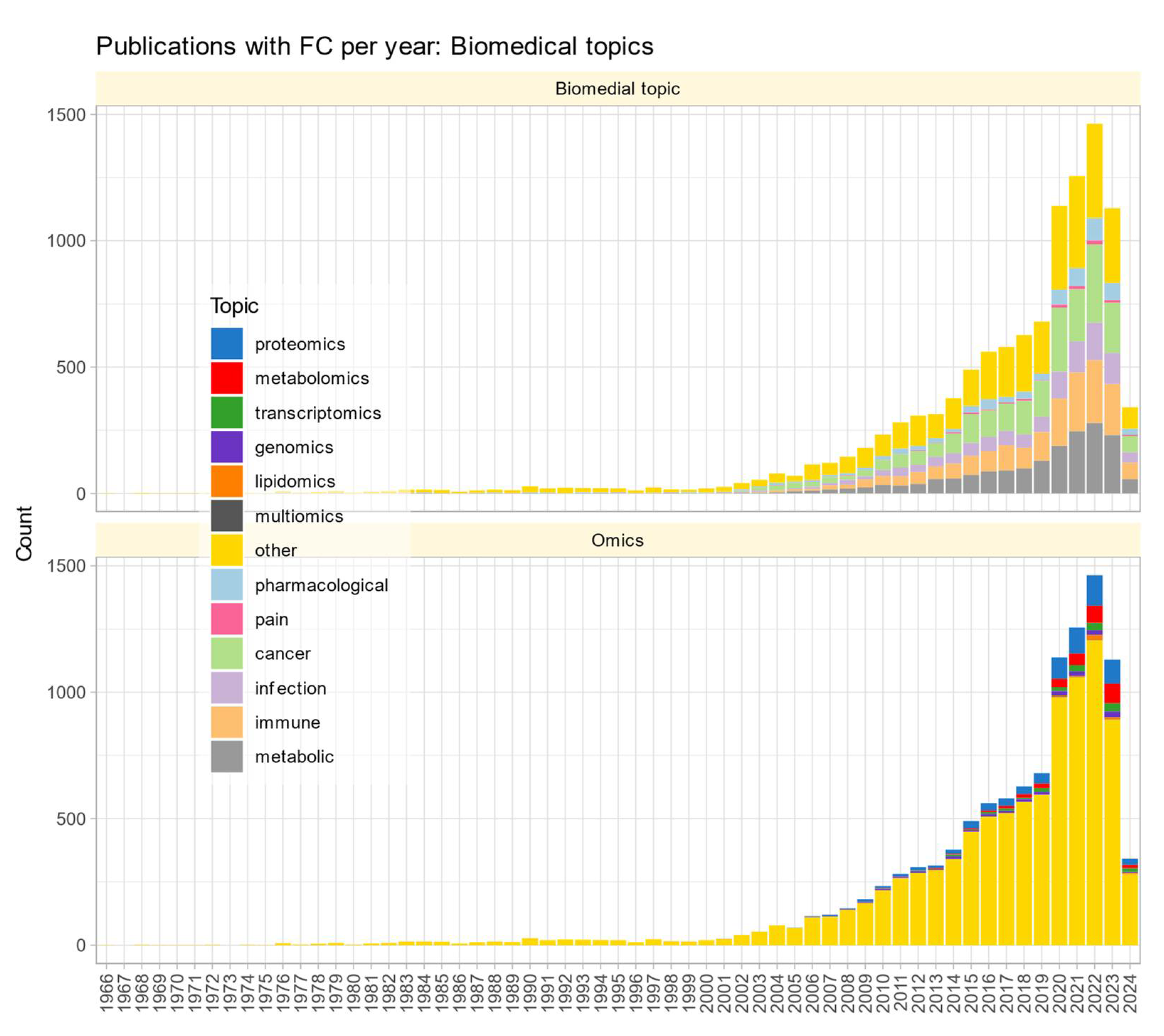
Fold change is widely used in biomedical research to quantify the magnitude of group differences in omics variables, initially mainly in gene expression studies but nowadays adopted in other "omics" fields and even non-omics research, as evidenced by a PubMed search for "fold change", where the term was found to be associated with a variety of fields beyond gene expression studies (Figure 1). Fold-change calculation can significantly influence the interpretation of results and subsequent decision-making processes in biomedical research. Gene lists from microarray studies generated by fold-change ranking were more reproducible than those obtained by t-test p-value or other significance analyses [1,2], and fold-change is a potential criterion for univariate feature selection [3], alone or as a complement to other machine learning-based methods for omics analysis [4].

Fold change is often visualized in "volcano plots" [5] using a

l o g 10 (p . v a l u e)

on the y-axis and log₂-ratio of signals between treatment and reference groups on the x-axis. However, the exact calculation method is often not reported, although several methods exist. The definition of “average” (such as arithmetic or geometric mean) to quantify group expression levels can lead to inconsistencies. Despite previous studies downplaying the consequences [5,6,7], it seems crucial to carefully choose the most robust method against potential violations of standard assumptions about the data distribution and variance. This report reevaluates the influence of various fold-change calculation methods on fold-change values and aims to recommend a preferred approach.

Methods

Retrieval of Fold Change Reporting in Biomedical Publications

On March 23, 2024, a PubMed (https://pubmed.ncbi.nlm.nih.gov/) search was performed using the query "("fold change" NOT (review[PT])". The R package "easyPubMed" (https://cran.r-project.org/package=easyPubMed [8]) was used to retrieve details of the papers, including titles, abstracts, and publication years. To identify the main topics where fold-change reporting is common, words in the abstracts were filtered against generic text using the R package ‘PubMedWordcloud’ (https://cran.r-project.org/package=PubMedWordcloud [9]). Recursive cABC analysis [10], an item categorization technique, was then applied to the frequency of the remaining words using the R library "ABCanalysis" (https://cran.r-project.org/package=ABCanalysis [11]). Biomedical domain experts identified biomedical topics based on the relevant terms. The type of omics research covered was determined by applying another cABC analysis to the occurrences of words containing the substring "omics".

Common Basic Variants of the Fold-Change Calculation

There are numerous descriptions of fold change calculation, such as in [12]. The calculation is based on the log ratio between the treatment and reference groups of a biological signal found in a dataset, i.e., the values of a variable of interest. One common way of calculating the signal log ratio is:

l o g R a t i o = {l o g}_{2} (\frac{E_{b, i}}{E_{a, i}}) = {l o g}_{2} (E_{b, i}) - {l o g}_{2} (E_{a, i})

Equation 1

where

E_{a, i}

and

E_{b, i}

are the positive, non-zero expected values of variable

i

measured under two different conditions a and b, such as before (

a

) and after (

b

) a treatment, or control (

a

) versus patient (

b

). The value of fold change,

F C

, is then obtained as [12]:

F C = \{\begin{matrix} 2^{l o g R a t i o} i f l o g R a t i o \geq 0 \\ {- 2}^{- l o g R a t i o} o t h e r w i s e \end{matrix}\}

Equation 2

Definition of Group Average from the Untransformed Data

There are several ways to define the expected values

E_{i}

for a variable. Often, the arithmetic mean is used and then Equation 1 becomes

l o g R a t i o = {l o g}_{2} (\bar{b_{i}} / \bar{a_{i}}) = {l o g}_{2} (\bar{b_{i}}) - {l o g}_{2} (\bar{a_{i}})

Equation 3

where the horizontal line placed over the variable, i.e.,

\bar{v}

, denotes the arithmetic mean of variable v.

Definition of Group Average from Transformed Data

For log-normally distributed data, the geometric mean serves as a more appropriate measure of central tendency compared to the arithmetic mean. The geometric mean effectively captures the expected value for positive log-normal distributed data, and its application in omics studies has been recommended [13]. It is calculated as the

n^{t h}

root of the product of

n

items

x

, i.e.,

\sqrt[n]{\prod_{i = 1}^{n} x_{i}}

, which in the log domain becomes arithmetic mean in log scale, i.e.,

{E_{x} = L o g}^{(\frac{1}{n} \sum_{i = 1}^{n} (\log_{\log} x_{i}))} = {L o g}^{\bar{\log x_{i}}}

. When also using 2 as the base of logarithm for calculating the log ratio for fold change as in Equation 1, the log ratio is then

{l o g R a t i o = l o g}_{2} (\frac{2^{\bar{\log_{2} b_{i}}}}{2^{\bar{\log_{2} a_{i}}}}) = {l o g}_{2} (2^{\bar{\log_{2} b_{i}} - \bar{\log_{2} a_{i}}}) = \bar{\log_{2} b_{i}} - \bar{\log_{2} a_{i}}

Equation 4

denoting the difference of the means of the logs of the two groups

b

and

a

Both calculation variants (i.e., calculating fold change via the log of the means as in Equation 3 or calculating it via the mean of the logs as in Equation 4) are in use. However, for log-normal distributed data, the log of the mean is in general not equal to the mean of the log-transformed data, i.e.,

{l o g}_{2} (\bar{x}) \neq \bar{{l o g}_{2} (x)}

and

F C \neq {F C}^{’}

for the values of fold-change obtained via the log ratios according to Equation 3 or Equation 4, respectively. Another measure of central tendency is the median, which is usually unaffected by the above discrepancy and was used for example in [14].

Pairwise Test/Reference Ratio Calculation

As an alternative approach, fold-change can be calculated by taking the ratio of each paired value from variable

b

and variable

a

. Let

A = \{a_{1}, a_{2}, \dots, a_{n}\}

be a vector of length

n_{a}

and

B = \{b_{1}, b_{2}, \dots, b_{n}\}

be a vector of length

n_{b}

. Then, for all possible combinations of an element of

A

with an element of

B

, expressed as

{p a i r s}_{a b} = \{(a, b)| a ϵ A, b ϵ B\}

, the log ratio can be calculated as:

l o g R a t i o = \bar{{l o g}_{2} (\frac{b_{i}}{a_{j}})} f o r ((a_{j}, b_{i}) ϵ {p a i r s}_{a b})

Equation 5

If the experimental design involves matched samples (e.g., before-and-after measurements, case-control studies), the case-wise calculation naturally incorporates this pairing. If some cases have missing values in either the treatment or reference group, the case-wise calculation can still proceed with the available pairings.

Comparative Evaluation of Common Calculation Methods

Evaluations were coded in the R language [15] using the R software package [16], version 4.4.0 for Linux (https://CRAN.R-project.org/), and in the matrix laboratory language using MATLAB (version 23.2.0.2485118 (R2023b)) and run on an AMD Ryzen Threadripper 3970X (Advanced Micro Devices, Inc., Santa Clara, CA, USA) desktop computer and an Intel® (Intel Corporation, Santa Clara, CA, USA) Core^TM i7-13700H notebook computer, both running on Ubuntu Linux 22.04.4 LTS (Canonical, London, UK). The equations used in the experiments are summarized in Table 1, along with the abbreviations or acronyms of the methods used in this report.

Evaluation of the Role of the Data Distribution for the Correct Calculation of FC

Fold change calculations were evaluated on data generated to represent different distributions, including normal and log-normal, as well as identity, uniform, and mixed, where the latter is a random mixture of the four former distributions (Data set # 1; Table 2). Two vectors

a

and

b

were created, with vector

a

with serving as the reference and the values of vector

b

being

F C

times the values of vector

a

. Thus, the ratios between

b

and

a

were known at the time of data generation allowing comparison of the

F C

values obtained by different calculation methods with the true values. Different combinations of

R a t i o = [\frac{1}{3}, 3]

with different standard deviations of the sample sizes of

a

and

b

were performed using different calculation methods of

F C

Evaluation of the Role of Variance Equality for the Correct Calculation of FC

Since the experiments above highlighted specific issues with the log-normal distribution for certain variants of

F C

calculation, and considering the frequent log-normal distribution of biological datasets, including non-omics data such as psychophysical measurements [17], and many others, the effect of different values of

F C

and different standard deviations of treatment (

s_{b}

) and reference (

s_{a}

)) on the accuracy of fold change recovery was explored in log-normally distributed data (Data set # 2). Across a wide range of simulated

F C = [0.1, \dots, 6]

and

\frac{s_{b}}{s_{a}} = [0.1,0 . 5,1, 2,4, 8]

= scenarios, with values of

s_{a} = [0.1,1]

, we quantified the errors in fold change estimates as

{E r r o r}_{F C} = s i g n (l o g ₂ ({F C}_{c a l c u l a t e d})) \cdot 2^{| l o g ₂ ({F C}_{c a l c u l a t e d}) |} - s i g n (l o g ₂ ({F C}_{t r u e})) \cdot 2^{| l o g ₂ ({F C}_{t r u e}) |}

Equation 6

Evaluation of the Relationship of FC Calculation to Statistical Outcomes

The two components of a volcano plot, fold change (

F C

) respectively the log ratio of treatment and reference and the statistical significance (

- \log_{10} p

), were further evaluated using a simulated dataset #3 containing variables with either normal or log-normal distributions. This dataset comprised 99 pairs of vectors,

a

(reference) and

b

(treatment), generated by randomly drawing values for means

m

, standard deviations

s_{a}

and

s_{b}

, and values of

F C

from predefined ranges. Different combinations of

R a t i o = [\frac{1}{3}, \dots, 3]

with different standard deviations

m_{l o g n o r m a l} = U_{1} (30,40), s_{a, b, l o g n o r m a l} = U_{2} (1,5), m_{n o r m a l} = U_{1} (500,600), s_{a, b, n o r m a l} = U_{2} (20,200)

. Experiments were conducted on these 99 pairs of vectors

a

and

b

, employing different calculations for

F C

(mean of logs, log of means, paired approach) in combination with both nonparametric (Wilcoxon-Mann-Whitney U test [18,19]) and parametric (t-test [20]) statistical methods for comparing the vectors

a

and

b

in each of the d = 99 variables. The correlations of the absolute values of

|F C|

with the values of

- \log_{10} (p)

were assessed by calculating Spearman’s

ρ

[21].

Evaluation of FC Calculation Method Dependency in Biomedical Data

Fold change calculations are widely available in the biomedical literature. Therefore, for the present reassessment of fold-change calculation methods, the analysis was limited to an extended multi-omics dataset (Data set # 3). It originates from recent rheumatologic research and consists of an ongoing omics study of a cohort clinically described in [22]. This cross-sectional study of patients with rheumatic diseases was conducted in accordance with the Declaration of Helsinki on Biomedical Research Involving Human Subjects and was approved by the Ethics Committee of the Medical Faculty of the Goethe University, Frankfurt am Main, Germany (approval number 19-492_5). Informed written consent was obtained from each participant. For the present analysis, a subset of cases consisting of n = 95 patients with psoriatic arthritis and n = 50 healthy controls have been used. The omics assessments included d = 680 plasma concentrations of d = 328 proteins from an inflammatory panel and d = 352 lipid markers.

Results

Reporting Styles of Fold-Change Calculation in Biomedical Publications

The search of the PubMed on March 23, 2024, using the query "("fold change" NOT (review[PT])" returned 10,978 results (Figure 1). However, the true prevalence of fold change reporting is likely much higher, as researchers often employ fold change calculations and visualizations without explicitly using the term in titles, keywords, or abstracts. The number of publications per year has been increasing steadily since the turn of the century. An analysis of the context in which

F C

reporting of omics research results is most common revealed five main biomedical topics (pharmacological research, cancer, infection, immune processes, metabolism) and seven variants of omics research (proteomics, metabolomics, transcriptomics, genomics, lipidomics, multiomics, toxicogenomics; Figure 1).

The exact calculation of fold-change (

F C

) values is rarely reported in the literature. A review of over 200 papers found that only about 5% mentioned the

F C

calculation method, often in the context of informatics approaches to differential expression analysis rather than the use of

F C

in reporting biomedical findings. Among the few relevant papers, some used the arithmetic mean [12,23], while others mentioned log transformation, hinting at the use of the geometric mean [24], though this was rarely stated explicitly. Additionally,

F C

is sometimes calculated from pre-transformed data, such as in the

2^{- Δ Δ C P}

method [25] as a standard in PCR data analysis [26].

Role of the Data Distribution for the Correct Calculation of FC

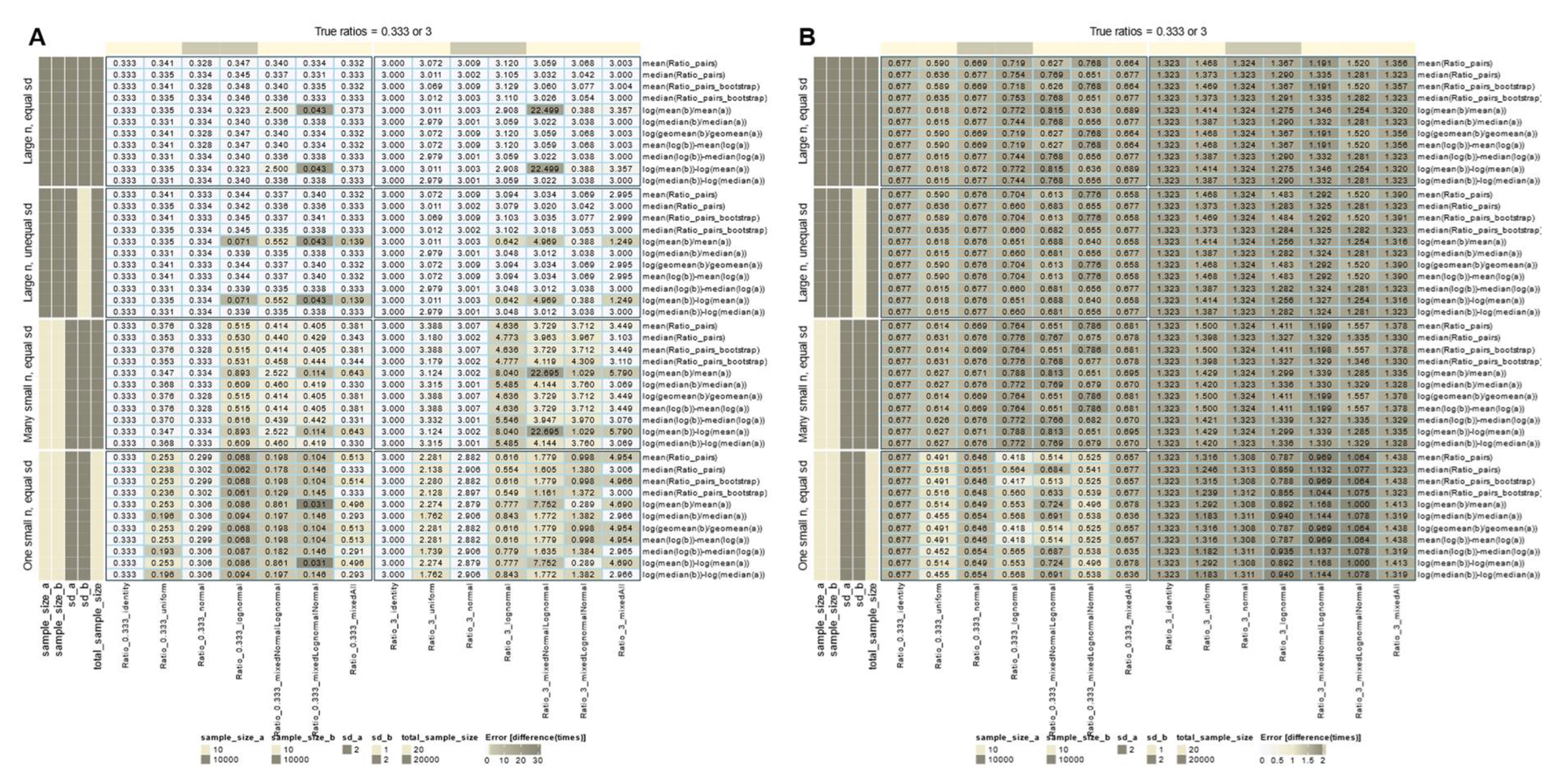
When the data distribution was normal, identity, or uniform, and the sample size was large (n = 10,000), all calculation methods accurately recovered the true treatment-to-reference ratios (Figure 2 A). However, when lognormal data were included, recovery was confounded by various conditions: most methods succeeded when the standard deviations of the treatment and reference groups were equal, except for the ratio of arithmetic means when the treatment and reference distributions were different. In contrast, all methods except the ratio of arithmetic means were robust to unequal variances. Recovery deteriorated drastically with small sample sizes, especially with lognormal data, and none of the methods provided accurate results. Repeating the experiments with small sample sizes slightly improved recovery for normal or identity distributions.

The intuitive use of fold-change assumes absolute expression levels. However, a pitfall arises when using pre-transformed data from standard workflows, without realizing it. Applying additional log-transformations means log-transforming already log-transformed data (Figure 2 B). Rankings of variables may be preserved, but calculated fold changes no longer represent "times expression", only arbitrary numbers, possibly better expressed as "times signal" as a more neutral description. When comparing studies or multi-omics data from different workflows, changes in fold change magnitude interpretation and comparability become relevant.

Role of Variance Equality for the Correct Calculation of FC

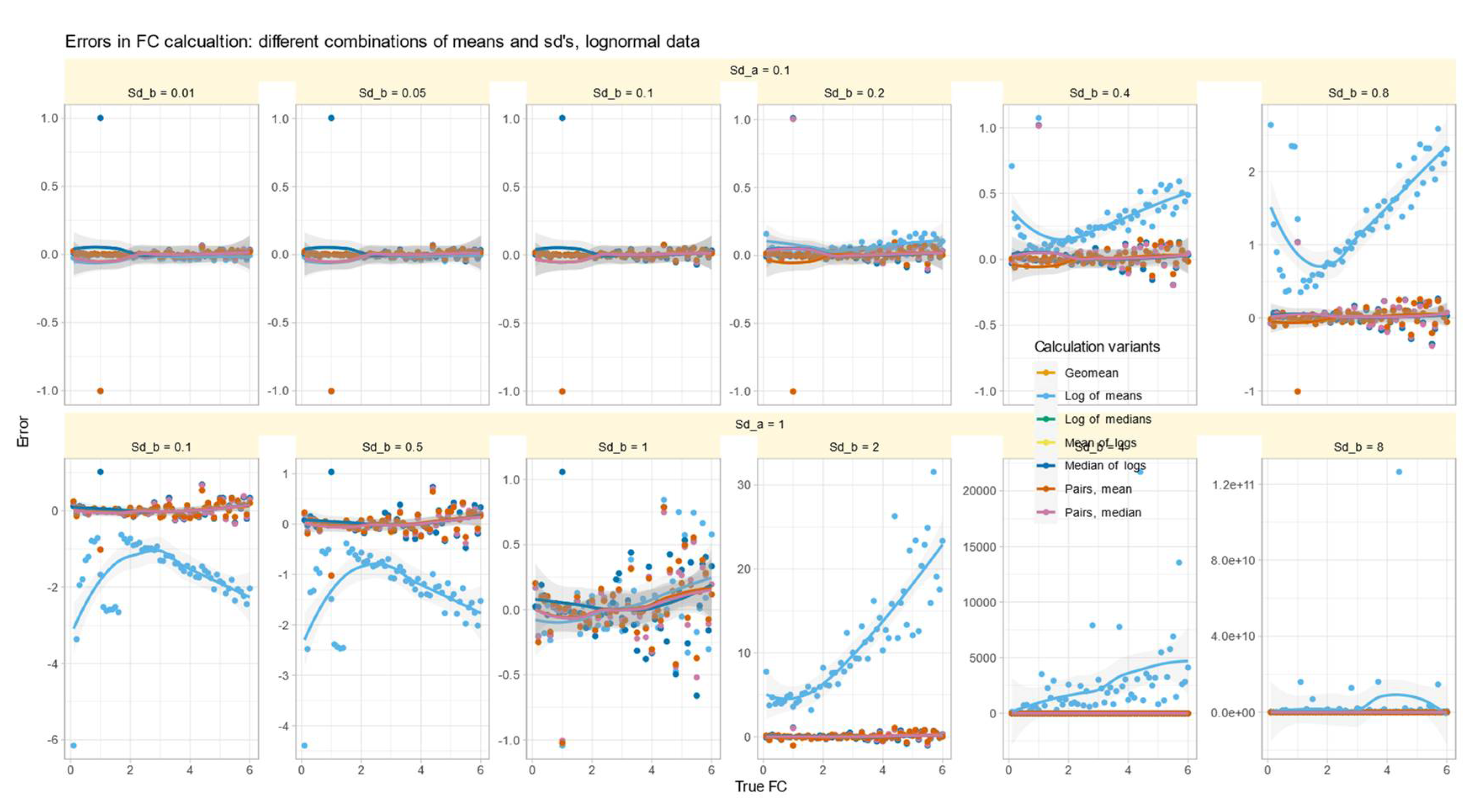
The errors in test/reference ratios calculated by major methods in Data Set #2 were analyzed for log-normal data with varying standard deviations. The results (Figure 3) showed that all methods except those based on arithmetic means made small errors of about 0.1 times more or less than the true factor. The arithmetic mean-based method had varying effects depending on the fold change and standard deviation of the test relative to the reference. Specifically, when

s_{b}

and

s_{a}

were not equal, the error reversed direction at a value of

F C = 1

. That is, when

s_{b} < s_{a}

and

F C < 1

, the arithmetic mean-based method overestimated the value of

F C

, was close to zero when

s_{b} ~ s_{a}

, and underestimated the error when

s_{b} > s_{a}

. Thus, the success of correctly estimating

F C

by arithmetic means depended first on the similarity of the standard deviations. This recalls a precondition of

F C

calculation mentioned in [5], namely that

F C

can be considered as the special case when the variances of all genes are equal.

Relationship between Calculated Fold Change and Statistical Significance

Intuitively, higher fold changes tend to be associated with higher statistical significance because larger expression differences between conditions are more likely to be statistically significant, assuming consistent variability within each condition. However, deviations from this intuitive expectation can occur due to high and different variability within and between conditions, leading to lower significance despite large fold changes.

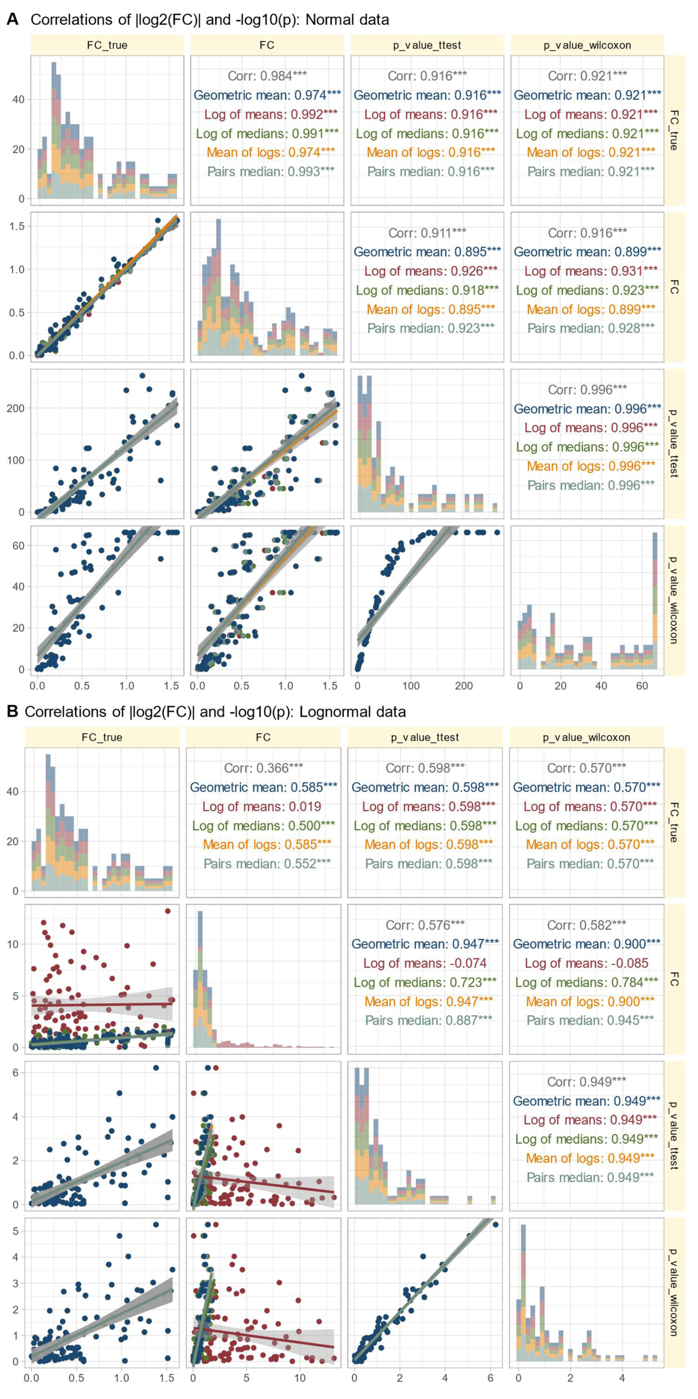
Data Set #3 tested the robustness of fold change (FC) calculation by combining different fold changes with varying standard deviations in normally and log-normally distributed data In normal distributed data, the choice of

F C

calculation method was nevertheless irrelevant to the results (Figure 4 A). The obtained values of

F C

correlated with the true values of

F C

and with the statistical significance of the group comparisons, and the correlations were quite similar regardless of the

F C

calculation method. The picture changed somewhat for log-normal data (Figure 4 B), where it became clear that calculating

F C

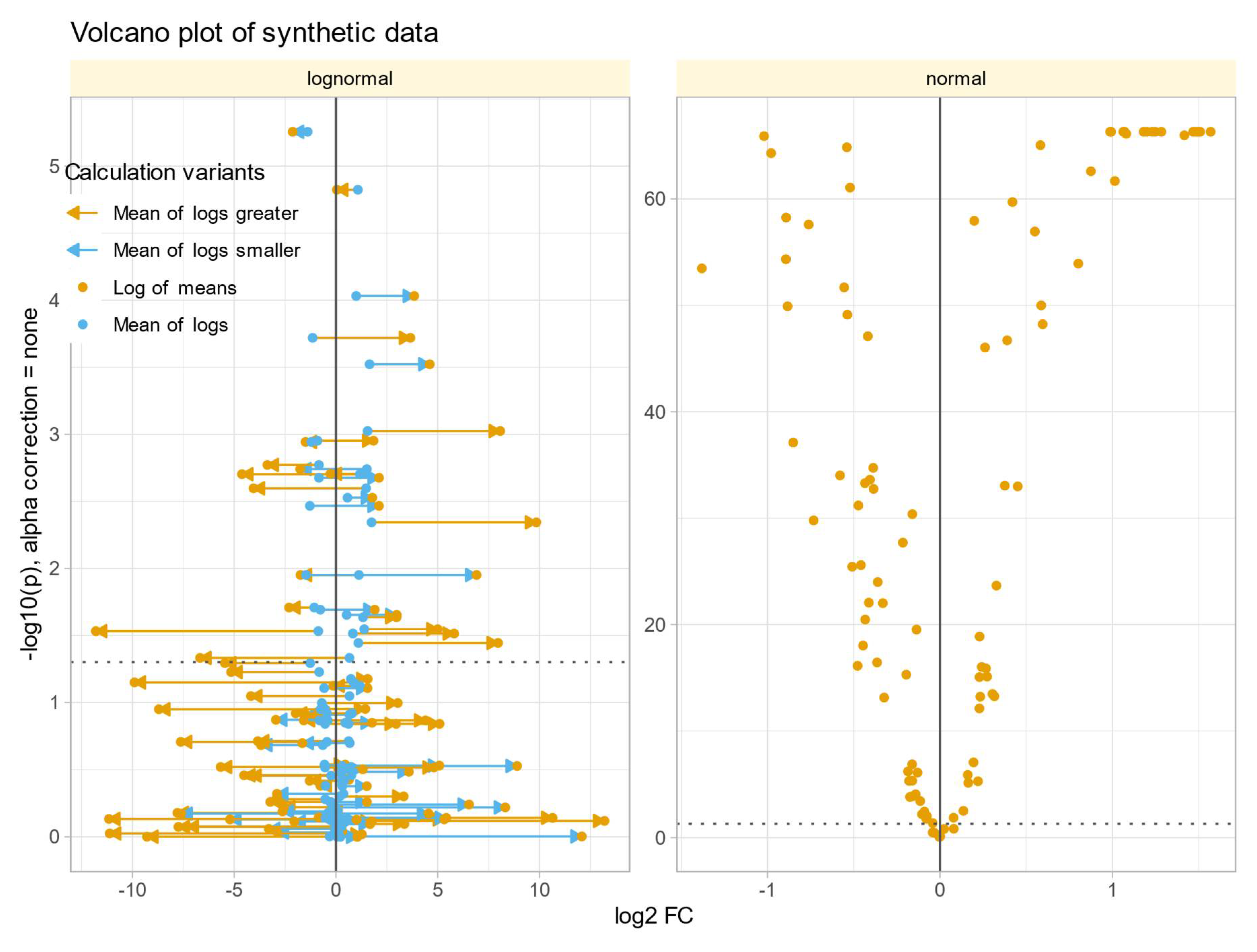
using the logarithm of the mean was associated with a higher risk of inaccuracy than the alternatives. This was evident in the volcano plot (Figure 5), where extreme cases showed crossover from downregulation to upregulation or vice versa.

FC Calculation Method Dependency in Biomedical Data

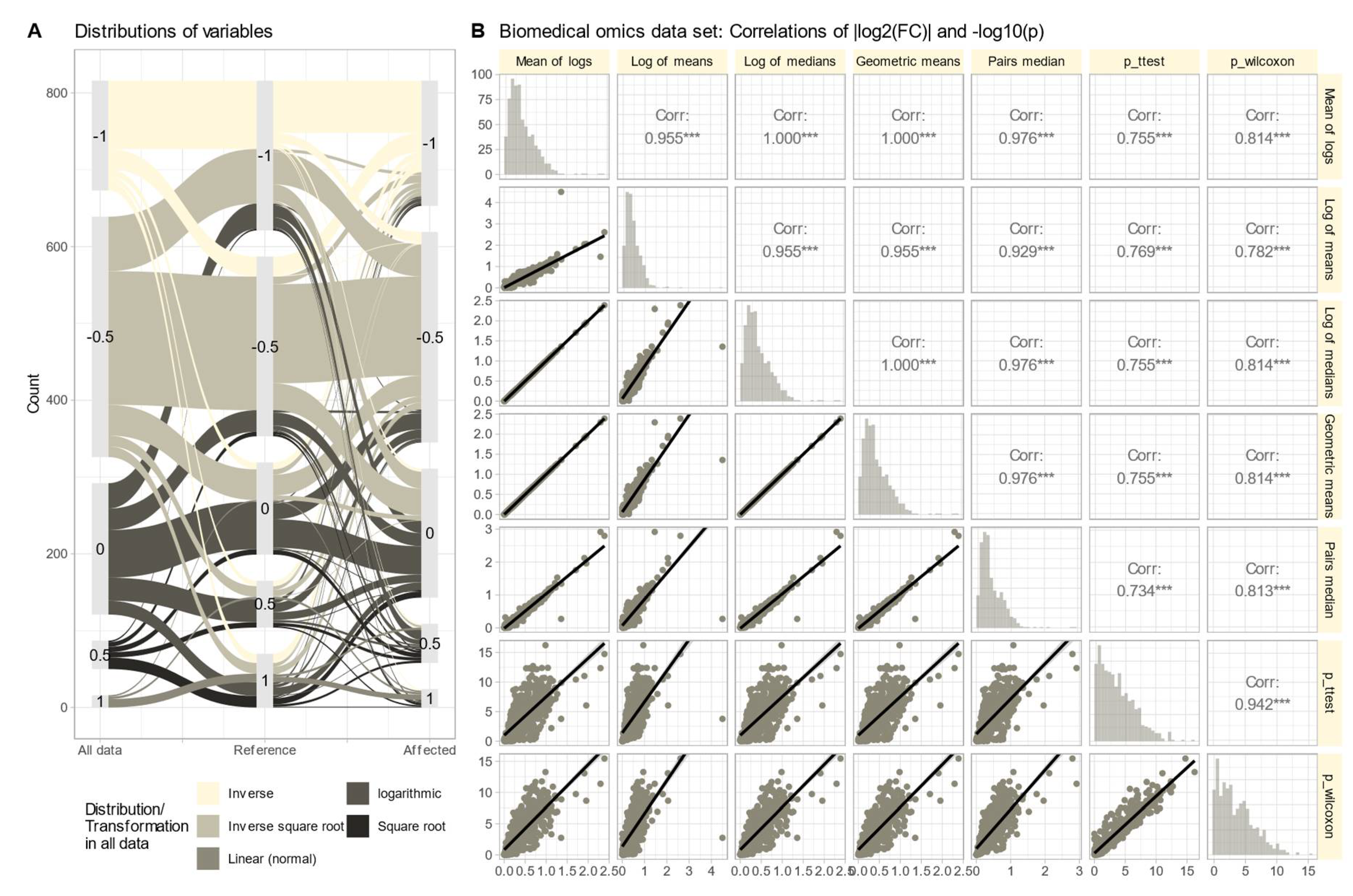
The omics data set #4 from rheumatology research showed diverse distributions, with only 14.3% of variables normally distributed in the raw data (Figure 6 A). Log-transforming the data increased normality to 48.1%. Therefore, Box-Cox transformation [27] was used with aligning the obtained values of

λ

with the steps of Tukey’s ladder of power [28]. The calculation of FC using different methods (logarithm of means, means of logs, etc.; Figure 6 B) yielded similar results, with high correlations between FC values and statistical significances in parametric and nonparametric tests. Further stressing of the calculations by complete permutation of the entire data matrices in the x- and y-directions resulted in highly skewed data (skewness = 23.4, kurtosis = 837.6). Then, the correlations between methods decreased, and the pairwise method showed the strongest correlation with nonparametric test results (Figure 7).

Discussion

Fold change calculation is widely used to describe the effect of a treatment on a measurement or group differences. Despite its ease of calculation, the exact method used is often not reported. Although different methods exist, they appear to give similar results. However, a re-evaluation of these methods found that one method, using the arithmetic mean, is less robust to anomalies in the data distribution and can result in incorrect fold change values more frequently than others. Unfortunately, this is often cited as the standard method for

F C

calculation [7,29].

The present experiments highlight the importance of sample size, distribution, and variance for accurate fold change calculation. For small sample sizes (e.g., n = 10), none of the methods could accurately reproduce true ratios. This limitation has been addressed in studies on sample size calculation for differential expression [30,31], but variance estimation from small samples can be generally unreliable [5]. In addition, if the

F C

calculation is considered as a special case when the variances of all genes are equal, the calculation via the supposed standard equation can go wrong. The present biomedical data showed different distributions of the test and reference data subsets (Figure 6 A), albeit to a degree that induced moderate consequences, but nevertheless show the possibility of such a scenario. The arithmetic mean fold change calculation was most sensitive to violations of assumptions, and the logarithmic calculation performed worst when data were log-normally distributed. In settings with unequal distributions, the arithmetic mean calculation diverged from true values, while alternative equations provided accurate results and maintained correlation with statistical significance.

In the present experiments, different mathematically identical calculation equation variants were used to improve clarity and serve as internal validation. However, we could not reproduce the distinction between

{F C}_{r a t i o}

and

{F C}_{d i f f e r e n c e}

made in previous work [7], as it seemed to interpret a difference as a ratio [32]. Here, we interpreted fold change exclusively as a ratio. Evaluations focused on calculating numerical fold change values without further refinement of up- or downregulation [33]. Comprehensive assessments highlight the need for more precise methods, especially for single-cell RNA-seq data [34], as the chosen statistical or fold change cutoff can provide multiple answers for microarray analysis [35].

Finally, the recommendation to use the median or geometric mean to quantify the expected value or group mean must be combined with the warning that even these values are not insensitive to unusual data constellations. The geometric mean is usually appropriate for lognormal data. The median is more general but can also be misleading. For example, in the analysis of right-skewed distributions observed in the analysis of social dynamics, the median can often be more misleading than the mean [36], and such scenarios are also not excluded in biomedical data. Above all, this simple example emphasizes that careful data exploration during preprocessing including the adequate visualization of raw data [37], as an essential part of the omics data analysis workflow, cannot be replaced by an unquestioned standard procedure rigidly applied to the data at hand.

The recommendation to use the median or geometric mean must be combined with the warning that these values are not insensitive to unusual data constellations. The geometric mean is usually appropriate for lognormal data, while the median can be misleading, especially for right-skewed distributions [36]. This emphasizes the importance of careful data exploration during preprocessing, including adequate visualization of raw data [37], as an essential part of the omics data analysis workflow that cannot be replaced by unquestioned standard procedures.

Conclusions

Fold change reporting is widely used to summarize differential expression patterns, but the exact calculation method is often unclear. Different equations can produce different results, especially when data distributions are unequal. To ensure accurate interpretation and reproducibility, it is crucial to use methods less sensitive to data distribution and accurately report the calculation methods used [38]. The inferior arithmetic mean-based method is often perceived as the standard, despite mathematically different equations being possible that mainly differ in the estimation of the expected value. In conclusion, the choice of fold-change calculation method can significantly influence the interpretation of results and subsequent decision-making processes in biomedical research. Adopting less vulnerable methods and transparent reporting is a reasonable practice to ensure correct interpretation and reproducibility.

Declarations

Ethics approval

The biomedical dataset has been acquired in a study that followed the recommendations of the Declaration of Helsinki on Biomedical Research Involving Human Subjects and was approved by the Ethics Committee of the Medical Faculty of the Goethe University, Frankfurt am Main, Germany (approval number 19-492_5)

Consent for Publication

Written informed consent, including anonymized publication, was obtained from all participants.

Author Contributions

Background, programming, execution of the experiments, writing of the manuscript, data analysis and preparation of figures, acquisition of funding. DK - Literature research and manuscript writing AU - Scientific advice, mathematical supervision, programming and execution of experiments, writing the manuscript.

Funding

JL was supported by the Deutsche Forschungsgemeinschaft (DFG Lo 612/16-1).

Data Availability Statement

The biomedical dataset used in the experiments in this report is available from the first author upon reasonable request and subject to approval by the appropriate ethics committee.

Conflicts of Interest

None declared.

References

Guo, L.; Lobenhofer, E.K.; Wang, C.; Shippy, R.; Harris, S.C.; Zhang, L.; Mei, N.; Chen, T.; Herman, D.; Goodsaid, F.M.; et al. Rat toxicogenomic study reveals analytical consistency across microarray platforms. Nat Biotechnol 2006, 24, 1162–1169. [Google Scholar] [CrossRef]
Dembélé, D.; Kastner, P. Fold change rank ordering statistics: a new method for detecting differentially expressed genes.
Guyon, I. An introduction to variable and feature selection. J. Mach. Learn. Res. 2003, 3, 1157–1182. [Google Scholar]
Cheng, J.; Liu, H.-P.; Lin, W.-Y.; Tsai, F.-J. Machine learning compensates fold-change method and highlights oxidative phosphorylation in the brain transcriptome of Alzheimer’s disease. Scientific Reports 2021, 11, 13704. [Google Scholar] [CrossRef] [PubMed]
Li, W. Volcano plots in analyzing differential expressions with mRNA microarrays. J Bioinform Comput Biol 2012, 10, 1231003. [Google Scholar] [CrossRef]
Dembélé, D.; Kastner, P. Fold change rank ordering statistics: a new method for detecting differentially expressed genes. BMC Bioinformatics 2014, 15, 14. [Google Scholar] [CrossRef] [PubMed]
Witten, D.; Tibshirani, R. A comparison of fold-change and the t-statistic for microarray data analysis. 1–17. 2007.
Fantini, D. easyPubMed: Search and Retrieve Scientific Publication Records from PubMed, 2019.
Fan, F.Y. PubMedWordcloud: ’Pubmed’ Word Clouds_. R package version 0.3.6, <https://CRAN.R-project.org/package=PubMedWordcloud>, 2019.
Lötsch, J.; Ultsch, A. Recursive computed ABC (cABC) analysis as a precise method for reducing machine learning based feature sets to their minimum informative size. Sci Rep 2023, 13, 5470. [Google Scholar] [CrossRef]
Ultsch, A.; Lötsch, J. Computed ABC Analysis for Rational Selection of Most Informative Variables in Multivariate Data. PLoS One 2015, 10, e0129767. [Google Scholar] [CrossRef] [PubMed]
Tadros, S.F.; D’Souza, M.; Zhu, X.; Frisina, R.D. Gene expression changes for antioxidants pathways in the mouse cochlea: relations to age-related hearing deficits. PLoS One 2014, 9, e90279. [Google Scholar] [CrossRef] [PubMed]
Olivier, J.; Johnson, W.D.; Marshall, G.D. The logarithmic transformation and the geometric mean in reporting experimental IgE results: what are they and when and why to use them? Ann Allergy Asthma Immunol 2008, 100, 333–337. [Google Scholar] [CrossRef] [PubMed]
Jain, N.; Thatte, J.; Braciale, T.; Ley, K.; O’Connell, M.; Lee, J.K. Local-pooled-error test for identifying differentially expressed genes with a small number of replicated microarrays. Bioinformatics 2003, 19, 1945–1951. [Google Scholar] [CrossRef] [PubMed]
Ihaka, R.; Gentleman, R. R: A Language for Data Analysis and Graphics. Journal of Computational and Graphical Statistics 1996, 5, 299–314. [Google Scholar] [CrossRef]
R Development Core Team. R: A Language and Environment for Statistical Computing. 2008.
Fechner, G.T. Elemente der Psychophysik; Breitkopf and Härtel: Leipzig, 1860. [Google Scholar]
Wilcoxon, F. Individual comparisons by ranking methods. Biometrics 1945, 1, 80–83. [Google Scholar] [CrossRef]
Mann, H.B.; Whitney, D.R. On a test of whether one of two random variables is stochastically larger than the other. Annals of Mathematical Statistics 1947, 18, 50–60. [Google Scholar] [CrossRef]
Student. The Probable Error of a Mean. Biometrika 1908, 6. [Google Scholar]
Spearman, C. The proof and measurement of association between two things. Am J Psychol 1904, 15, 72–101. [Google Scholar] [CrossRef]
Rischke, S.; Poor, S.M.; Gurke, R.; Hahnefeld, L.; Köhm, M.; Ultsch, A.; Geisslinger, G.; Behrens, F.; Lötsch, J. Machine learning identifies right index finger tenderness as key signal of DAS28-CRP based psoriatic arthritis activity. Sci Rep 2023, 13, 22710. [Google Scholar] [CrossRef]
Kumar, N.; Hoque, M.A.; Sugimoto, M. Robust volcano plot: identification of differential metabolites in the presence of outliers. BMC Bioinformatics 2018, 19, 128. [Google Scholar] [CrossRef] [PubMed]
Hauber, A.L.; Rosenblatt, M.; Timmer, J. Uncovering specific mechanisms across cell types in dynamical models. PLoS Comput Biol 2023, 19, e1010867. [Google Scholar] [CrossRef] [PubMed]
Livak, K.J.; Schmittgen, T.D. Analysis of relative gene expression data using real-time quantitative PCR and the 2(-Delta Delta C(T)) Method. Methods 2001, 25, 402–408. [Google Scholar] [CrossRef] [PubMed]
Fu, W.J.; Hu, J.; Spencer, T.; Carroll, R.; Wu, G. Statistical models in assessing fold change of gene expression in real-time RT-PCR experiments. Comput Biol Chem 2006, 30, 21–26. [Google Scholar] [CrossRef] [PubMed]
Box, G.E.; Cox, D.R. An analysis of transformations. Journal of the Royal Statistical Society. Series B (Methodological) 1964, 211–252. [Google Scholar] [CrossRef]
Tukey, J.W. Exploratory Data Analysis; Addison-Wesley: Reading, Mass, 1977. [Google Scholar]
Tusher, V.G.; Tibshirani, R.; Chu, G. Significance analysis of microarrays applied to the ionizing radiation response. Proc Natl Acad Sci U S A 2001, 98, 5116–5121. [Google Scholar] [CrossRef] [PubMed]
Li, C.I.; Su, P.F.; Shyr, Y. Sample size calculation based on exact test for assessing differential expression analysis in RNA-seq data. BMC Bioinformatics 2013, 14, 357. [Google Scholar] [CrossRef] [PubMed]
Bi, R.; Liu, P. Sample size calculation while controlling false discovery rate for differential expression analysis with RNA-sequencing experiments. BMC Bioinformatics 2016, 17, 146. [Google Scholar] [CrossRef] [PubMed]
Choe, S.E.; Boutros, M.; Michelson, A.M.; Church, G.M.; Halfon, M.S. Preferred analysis methods for Affymetrix GeneChips revealed by a wholly defined control dataset. Genome Biology 2005, 6, R16. [Google Scholar] [CrossRef] [PubMed]
Newton, M.A.; Kendziorski, C.M.; Richmond, C.S.; Blattner, F.R.; Tsui, K.W. On Differential Variability of Expression Ratios: Improving Statistical Inference about Gene Expression Changes from Microarray Data. Journal of Computational Biology 2001, 8, 37–52. [Google Scholar] [CrossRef] [PubMed]
Wang, T.; Li, B.; Nelson, C.E.; Nabavi, S. Comparative analysis of differential gene expression analysis tools for single-cell RNA sequencing data. BMC Bioinformatics 2019, 20, 40. [Google Scholar] [CrossRef] [PubMed]
Dalman, M.R.; Deeter, A.; Nimishakavi, G.; Duan, Z.H. Fold change and p-value cutoffs significantly alter microarray interpretations. BMC Bioinformatics 2012, 13 Suppl 2, S11. [Google Scholar] [CrossRef]
Kämpke, T. The use of mean values vs. medians in inequality analysis. Journal of economic and social measurement 2010, 35, 43–62. [Google Scholar] [CrossRef]
Lötsch, J.; Ultsch, A. Comments on the importance of visualizing the distribution of pain-related data. European journal of pain (London, England). [CrossRef]
National Academies of Sciences, E.; Medicine; Policy; Global, A.; Committee on Science, E.M.; Public, P.; Board on Research, D.; Information; Division on, E.; Physical, S.; et al. In Reproducibility and Replicability in Science; National Academies Press (US): Washington (DC), 2019.
Wickham, H. ggplot2: Elegant Graphics for Data Analysis; Springer-Verlag New York: 2009.
Gu, Z.; Eils, R.; Schlesner, M. Complex heatmaps reveal patterns and correlations in multidimensional genomic data. Bioinformatics 2016, 32, 2847–2849. [Google Scholar] [CrossRef] [PubMed]
Schloerke, B.; Crowley, J.; Cook, D.; Briatte, F.; Marbach, M.; Thoen, E.; Elberg, A.; Larmarange, J. GGally: Extension to ’ggplot2’, 2018.
Pedersen, T.L. ggforce: Accelerating ’ggplot2’, 2020.

Figure 1. Stacked bar chart of the number of publications per year according to a simple query of PubMed (https://pubmed.ncbi.nlm.nih.gov/) for "("fold change" NOT (review[PT])" on March 23, 2024. The top panel shows the biomedical topic according to an article categorization of the most frequent biomedical contexts of fold change mention. The lower part shows the same for the term "omics" in the titles, keywords or abstracts of the hits. The figure has been created using the software package R (version 4.4.0 for Linux; https://CRAN.R-project.org/ [16]) and the library "ggplot2" (https://cran.r-project.org/package=ggplot2 [39]).

Figure 2. Recovery of fold-change values used to generate artificial data (data set #1) with different distributions (identical, uniform, normal, lognormal), including mixed distributions such as "mixed", i.e. a mixture of all four distributions mentioned, or "mixedNormalLognormal" (treatment: normal, reference: lognormal) or "mixedlognormalNormal" (treatment: lognormal, reference: normal). The fold change calculations are shown on the right and were performed using different methods as specified in Table 1. A: calculations without further data transformation. B: All data were again log-transformed, regardless of their original distribution. The figure has been created using the R software package (version 4.4.0 for Linux; https://CRAN.R-project.org/ [16]) and the R libraries "ggplot2" (https://cran.r-project.org/package=ggplot2 [39]) and “ComplexHeatmap” (https://www.bioconductor.org/packages/ComplexHeatmap/ [40]).

Figure 3. Errors of fold change recovery from synthetic data (data set #2) generated along a range of fold change values of

F C = [0.1, \dots, 6]

with standard deviation of reference of

s_{a} = 0.1

(upper line of panels) and

s_{a} = 1

(lower line of panels) and standard deviations of the treatment subgroup (

s_{b}

) at ratios

\frac{s_{b}}{s_{a}} = [. 1, . 5,1, 2,4, 8]

(panels form left to right). The trends of the relations are shown as linear regression lines with 95% confidence intervals of the fits. The fold change calculations were performed using different methods as specified in Table 1. The figure has been created using the R software package (version 4.4.0 for Linux; https://CRAN.R-project.org/ [16]) and the R libraries "ggplot2" (https://cran.r-project.org/package=ggplot2 [39])

Figure 3. Errors of fold change recovery from synthetic data (data set #2) generated along a range of fold change values of

F C = [0.1, \dots, 6]

with standard deviation of reference of

s_{a} = 0.1

(upper line of panels) and

s_{a} = 1

(lower line of panels) and standard deviations of the treatment subgroup (

s_{b}

) at ratios

\frac{s_{b}}{s_{a}} = [. 1, . 5,1, 2,4, 8]

Figure 4. Correlations of |log2(FC)| and -log10(p) in synthetic data (data set #3) with normal (top) or lognormal (bottom) distribution. Each d = 99 treatment and reference data sets were generated by randomly assigning fold-change values and treatment (

s_{b}

) and reference (

s_{a}

) standard deviations from predefined ranges. The trends of the relations are shown as linear regression lines with 95% confidence intervals of the fits. The diagonal shows stacked histograms of the distributions of the respective values. "FC_true" denotes the absolute value of the log2 treatment/reference ratio used during data generation, i.e. |logs(FC)|, "FC" denotes the same for the value calculated according to different equations. The upper right triangle shows the Spearman’s correlation coefficient

ρ

with stars indicating the significance level (* = p <0.05, **: p <0.01, ***: p < 0.001). The fold change calculations were performed using different methods as specified in Table 1. The figure has been created using the R software package (version 4.4.0 for Linux; https://CRAN.R-project.org/ [16]) and the R libraries "ggplot2" (https://cran.r-project.org/package=ggplot2 [39]) and “GGally” (https://cran.r-project.org/package=GGally [41]).

s_{b}

) and reference (

s_{a}

ρ

Figure 5. Volcano plots of synthetic data (data set #3) with lognormal (left panel) or normal (right panel) distribution, obtained when fold changes were estimated using either "log of means": calculation using the arithmetic mean as the definition of the expected or average value of each subgroup (Equation 3) or the "mean of logs": calculation using the arithmetic mean of the logs of treatment and reference as the definition of the expected or average value of each subgroup (identical to "Geomean"; Equation 4). The lines connect the points on the diagram that represent the same variables with

F C

calculated by either method. The ordinate displays

- l o g 10 ({p_v a l u e s}_{W i l c o x o n t e s t})

without α-correction. The figure has been created using the R software package (version 4.4.0 for Linux; https://CRAN.R-project.org/ [16]) and the R library "ggplot2" (https://cran.r-project.org/package=ggplot2 [39]).

F C

calculated by either method. The ordinate displays

- l o g 10 ({p_v a l u e s}_{W i l c o x o n t e s t})

Figure 6. Untransformed real-life omics data (proteomics, lipidomics; data set #4). A: Distribution of variables according to the

λ

of the Box-Cox analysis. Sankey plot showing the distribution of variables (i) in the complete data and separately for (ii) reference and (iii) treatment subgroups. B: Correlations of |log2(FC)| and -log10(p) in untransformed real-life omics data (proteomics, lipidomics) after complete permutation of the 2D-matric in x and y direction. The trends of the relations are shown as linear regression lines with 95% confidence intervals of the fits. The diagonal shows stacked histograms of the distributions of the respective values. The upper right triangle shows the Spearman’s correlation coefficient

ρ

with stars indicating the significance level (* = p <0.05, **: p <0.01, ***: p < 0.001). The fold change calculations were performed using different methods as specified in Table 1. The figure has been created using the R software package (version 4.4.0 for Linux; https://CRAN.R-project.org/ [16]) and the R libraries "ggplot2" (https://cran.r-project.org/package=ggplot2 [39]), “GGally” (https://cran.r-project.org/package=GGally [41]) and “ggforce” (https://cran.r-project.org/package=ggforce [42]).

Figure 6. Untransformed real-life omics data (proteomics, lipidomics; data set #4). A: Distribution of variables according to the

λ

ρ

with stars indicating the significance level (* = p <0.05, **: p <0.01, ***: p < 0.001). The fold change calculations were performed using different methods as specified in Table 1. The figure has been created using the R software package (version 4.4.0 for Linux; https://CRAN.R-project.org/ [16]) and the R libraries "ggplot2" (https://cran.r-project.org/package=ggplot2 [39]), “GGally” (https://cran.r-project.org/package=GGally [41]) and “ggforce” (https://cran.r-project.org/package=ggforce [42]).

Figure 7. Correlations of |log2(FC)| and -log10(p) in untransformed real-life omics data (proteomics, lipidomics) after complete permutation of the 2D-matric in x and y direction. The trends of the relations are shown as linear regression lines with 95% confidence intervals of the fits. The diagonal shows stacked histograms of the distributions of the respective values. The upper right triangle shows the Spearman’s correlation coefficient

ρ

ρ

Table 1. Calculation of log ratios between treatment/test (

b

) and reference (

a

). The left column gives the short names with equations indicated, the middle column the short names or descriptions used throughout the report, including in the figures, and the right column gives the calculations performed. The right column refers to the calculation method to the corresponding equation number in this report.

Table 1. Calculation of log ratios between treatment/test (

b

) and reference (

a

Definition of expected value	Equation name	Short name	Calculation	Equation #
Mean	log(mean(b)/mean(a))	Log of means	$l o g R a t i o = {l o g}_{2} (\bar{b_{i}} / \bar{a_{i}})$	Equation 3
Mean	log(mean(b))-log(mean(a))	Log of means	$l o g R a t i o = {l o g}_{2} (\bar{b_{i}}) - {l o g}_{2} (\bar{a_{i}})$	Equation 3
Median	log(median(b)/median(a))	Log of medians	$l o g R a t i o = {l o g}_{2} (\tilde{b_{i}} / \tilde{a_{i}})$	Like Equation 3 but median
Median	log(median(b))-log(median(a))	Log of medians	$l o g R a t i o = {l o g}_{2} (\tilde{b_{i}}) - {l o g}_{2} (\tilde{a_{i}})$	Like Equation 3 but median
Geometric mean	log(geomean(b)/geomean(a))	Geometric mean	${l o g R a t i o = l o g}_{2} (\frac{2^{\bar{\log_{2} b_{i}}}}{2^{\bar{\log_{2} a_{i}}}})$	Equation 4
Geometric mean	mean(log(b))-mean(log(a))	Mean of logs	$l o g R a t i o = \bar{\log_{2} b_{i}} - \bar{\log_{2} a_{i}}$	Equation 4
Mean of logs	median(log(b))-median(log(a))	Median of logs	$l o g R a t i o = \tilde{\log_{2} b_{i}} - \tilde{\log_{2} a_{i}}$	Like Equation 4 but median
Paired fold change combinations	mean(Ratio_pairs)	Pairs mean	$l o g R a t i o = \bar{{l o g}_{2} (\frac{b_{i}}{a_{j}})} f o r ((a_{j}, b_{i}) ϵ {p a i r s}_{a b})$	Equation 5
Paired fold change combinations	median(Ratio_pairs)	Pairs median	$l o g R a t i o = \tilde{{l o g}_{2} (\frac{b_{i}}{a_{j}})} f o r ((a_{j}, b_{i}) ϵ {p a i r s}_{a b})$	Like Equation 5 but median
Paired fold change combinations	mean(Ratio_pairs_bootstrap)	Pairs mean bootstrap	$l o g R a t i o = \bar{{l o g}_{2} (\frac{b_{i}^{}}{a_{j}^{}})} f o r ((a_{j}, b_{i}) ϵ {b o o t s t r a p p e d p a i r s}_{a b}^{*})$	Like Equation 5 but bootstrapped pairs
Paired fold change combinations	mean(Ratio_pairs_bootstrap)	Pairs median boostrap	$l o g R a t i o = \tilde{{l o g}_{2} (\frac{b_{i}^{}}{a_{j}^{}})} f o r ((a_{j}, b_{i}) ϵ {b o o t s t r a p p e d p a i r s}_{a b}^{*})$	Like Equation 5 but bootstrapped pairs

Table 2. Artificial data sets created to assess certain effects of data distribution on the correct recovery of

F C

values by different calculation methods. All data sets contained vectors

a

and

b

were created, with vector

a

with serving as the reference and the values of vector

b

being

F C

times the values of vector

a

. That is, vector

a

had a mean, if applicable, of

m_{a} = m

, a standard deviation, if applicable, of

s_{a}

, and a sample size of

n_{a}

. Vector

b

had a mean of

m_{b} = F C \cdot m_{a}

, a standard deviation of

s_{b}

, and a sample size of

n_{b}

U_{1}

and

U_{2}

denote independent uniform distributions and

N

denotes the normal distribution.

Table 2. Artificial data sets created to assess certain effects of data distribution on the correct recovery of

F C

values by different calculation methods. All data sets contained vectors

a

and

b

were created, with vector

a

with serving as the reference and the values of vector

b

being

F C

times the values of vector

a

. That is, vector

a

had a mean, if applicable, of

m_{a} = m

, a standard deviation, if applicable, of

s_{a}

, and a sample size of

n_{a}

. Vector

b

had a mean of

m_{b} = F C \cdot m_{a}

, a standard deviation of

s_{b}

, and a sample size of

n_{b}

U_{1}

and

U_{2}

denote independent uniform distributions and

N

denotes the normal distribution.

Data set	Distribution	Generation
Data set #1	Identity	$a = \underset{n_{a}}{\underset{⏟}{m_{a}, m_{a}, \dots, m_{a}}}$ $b = F C \cdot \underset{n_{b}}{\underset{⏟}{m_{a}, m_{a}, \dots, m_{a}}}$
	Uniform	${a = U}_{1} (n_{a}, 0,1) \cdot m_{a}$ ${b = U}_{2} (n_{b}, 0,1) \cdot m_{a} \cdot F C$
	Normal	$a = a_{1}, a_{2}, \dots, a_{n_{a}} ~ N (m_{a}, s_{a})$ $b = b_{1}, b_{2}, \dots, b_{n_{b}} ~ N ({F C \cdot m}_{a}, s_{b})$
	Log-normal	$a = a_{1}, a_{2}, \dots, a_{n_{a}} ~ L o g N o r m a l (\log (m_{a}), s_{a})$ $b = b_{1}, b_{2}, \dots, b_{n_{b}} ~ L o g N o r m a l (\log (FC) + \log (m_{a}), s_{b})$
	mixedNormalLognormal	$a = a_{1}, a_{2}, \dots, a_{n_{a}} ~ N (m_{a}, s_{a})$ $b = b_{1}, b_{2}, \dots, b_{n_{b}} ~ L o g N o r m a l (\log (FC) + \log (m_{a}), s_{b})$
	mixedLogormalNormal	$a = a_{1}, a_{2}, \dots, a_{n_{a}} ~ L o g N o r m a l (\log (m_{a}), s_{a})$ $b = b_{1}, b_{2}, \dots, b_{n_{b}} ~ N ({F C \cdot m}_{a}, s_{b})$
	Mixed	$a = U_{1} \underset{n_{a}}{\underset{⏟}{\{\{a_{I d e n t i t y}\}, \{a_{U n i f o r m}\}, \{a_{N o r m a l}\}, \{a_{L o g - n o r m a l}\}\}}}$ $b = U_{2} \underset{n_{b}}{\underset{⏟}{\{\{b_{I d e n t i t y}\}, \{b_{U n i f o r m}\}, \{b_{N o r m a l}\}, \{b_{L o g - n o r m a l}\}\}}}$
Data set #2	Log-normal	$a = a_{1}, a_{2}, \dots, a_{n_{a}} ~ L o g N o r m a l (\log (m_{a}), s_{a})$ $b = b_{1}, b_{2}, \dots, b_{n_{b}} ~ L o g N o r m a l (\log (FC) + \log (m_{a}), s_{b})$
Data set #3	Normal	$a ~ N (m, s_{a})$ $b ~ N (F C \cdot m, s_{b})$
	Log-normal	$a ~ L o g N o r m a l (\log (m), s_{a})$ $b ~ L o g N o r m a l (\log (F C) + \log (m), s_{b})$

Disclaimer/Publisher’s Note: The statements, opinions and data contained in all publications are solely those of the individual author(s) and contributor(s) and not of MDPI and/or the editor(s). MDPI and/or the editor(s) disclaim responsibility for any injury to people or property resulting from any ideas, methods, instructions or products referred to in the content.

© 2024 by the authors. Licensee MDPI, Basel, Switzerland. This article is an open access article distributed under the terms and conditions of the Creative Commons Attribution (CC BY) license (http://creativecommons.org/licenses/by/4.0/).

Copyright: This open access article is published under a Creative Commons CC BY 4.0 license, which permit the free download, distribution, and reuse, provided that the author and preprint are cited in any reuse.

MDPI Initiatives

Important Links

Choose an area of interest and we will send you notifications of new preprints at your preferred frequency.

Disclaimer

Revisiting Fold-Change Calculation: Preference for Median or Geometric Mean over Arithmetic Mean-Based Methods

Abstract

Introduction

Methods

Retrieval of Fold Change Reporting in Biomedical Publications

Common Basic Variants of the Fold-Change Calculation

Definition of Group Average from the Untransformed Data

Definition of Group Average from Transformed Data

Pairwise Test/Reference Ratio Calculation

Comparative Evaluation of Common Calculation Methods

Evaluation of the Role of the Data Distribution for the Correct Calculation of FC

Evaluation of the Role of Variance Equality for the Correct Calculation of FC

Evaluation of the Relationship of FC Calculation to Statistical Outcomes

Evaluation of FC Calculation Method Dependency in Biomedical Data

Results

Reporting Styles of Fold-Change Calculation in Biomedical Publications

Role of the Data Distribution for the Correct Calculation of FC

Role of Variance Equality for the Correct Calculation of FC

Relationship between Calculated Fold Change and Statistical Significance

FC Calculation Method Dependency in Biomedical Data

Discussion

Conclusions

Declarations

Ethics approval

Consent for Publication

Author Contributions

Funding

Data Availability Statement

Conflicts of Interest

References

MDPI Initiatives

Important Links

Subscribe