1. Introduction
The main focus of this work is on the use of coil springs in the suspension systems of passenger cars. However, the same approaches may be used to evaluate springs in many applications by adapting them to account for the particular differences inherent in each application. While there are several ideas related to Digital Twin (DT), the use of live simulation for the purpose of enhancing condition monitoring and maintenance remains relatively underdeveloped. The phrase "(Digital) Twin" was first suggested by Michael Grieves in 2002 within the framework of Product Lifecycle Management (PLM). The Whitepaper, authored by Grieves in the same year [
1], provides a definition of Digital Twin (DT) as a duplicate of a real-world physical system. Grieves outlines three elements of this replication, namely: (A) the physical entity, (B) the digital counterpart, and (C) the connection between the physical and digital components. Nevertheless, the aforementioned description lacks the necessary formality to be considered a formal definition. Additionally, it fails to include the crucial aspects of data and services that have a significant influence on the effectiveness and precision of the model. In 2005, Grieves provided a comprehensive analysis of his conceptualization of Design Thinking (DT), which was first proposed in 2002. Grieves categorized DT into three distinct forms, namely: (A) DT prototype, (B) DT aggregate, and (C) DT instance [
2].
In 2010, the National Aeronautics and Space Administration (NASA) established a definition for Digital Transformation (DT) within the context of modelling, simulation, information technology, and processing roadmap [
3]. During the period from 2005 to 2010, a number of technological advancements were implemented, including the integration of Digital Twin (DT) technology into the structural management systems of aircraft by organizations such as NASA and the US Air Force. In the year 2018, the renowned worldwide research and consulting business known as Gartner officially recognized Digital Transformation (DT) as one of the ten most promising technologies for the future [
1]. The regular maintenance of mechanical services is of utmost importance for ensuring their dependability and safety. Engineers are responsible for ensuring that all operational components are maintained in optimal working conditions. While there is a cost associated with preventative maintenance, the alternative of replacing failing components after failure or servicing parts sooner than necessary might result in avoidable delays and increased prices [
4]. The presence of malfunctioning machinery disrupts the established schedules and impedes the progress of manufacturing lines. Therefore, in order to ensure the dependability and security of continuous and prosperous production line operations, operators must prioritize maintenance. The study conducted by Wyman in 2019 revealed that maintenance expenses account for over 30% of overall life costs. Consequently, a diverse array of computerized solutions has been developed to facilitate efficient maintenance management. Utilizing conventional simulation approaches that use fixed data to apply simplistic models is deemed inadequate for efficient maintenance practices, since it fails to account for the dynamic degradation of current temporal sections [
5].
Nevertheless, the use of up-to-date temporal data will provide a more comprehensive understanding of prevailing circumstances. The Twin (DT) is an emerging informatics technology that relies on the Internet of Things (IoT). Despite its growing popularity, there is a lack of consensus among writers about the precise definition and conceptualization of the DT [
6,
7,
8]. The technologies of Digital Twins (DTs) have garnered considerable attention in the public sphere. However, it is worth noting that the research conducted on DTs lacks transparency, despite the substantial efforts made and the potential they have for facilitating the integration of DTs into many businesses [
9]. The understanding of the notion of DT is now limited, hence exerting an influence on the prospective advancement of DT technology. Prominent sectors such as the automobile industry and the oil and gas sector were compelled to explore the notion of digital twins and undertake their implementation in relation to their respective goods and services [
10]. Additionally, the real-time visualization of the geometry and behavioural components of the systems has not yet been achieved. These components serve as access points for monitoring the various features of the system. This paper utilizes a case study of a suspension system to illustrate the proposed Dynamic Time Model (DTM) for real-time condition monitoring and predictive maintenance.
The case study also highlights the potential failure caused by fatigue when the suspension system, specifically the coil spring, is exposed to varying levels of loading over time. The coil spring experiences significant strain due to the cyclic load, leading to the need for fatigue life evaluation. Currently, simulations are being conducted to forecast the fatigue damage of the coil spring. The data acquired on load and strain presents a viable method for incorporation into the real-time simulation. This simulation assesses the fatigue, load, and strain experienced by the suspension system throughout its lifespan, using strain and load sensors that operate in conjunction with the server's data at the present moment.
1.1. Coil Springs Maintenance
Coiled springs are an essential component of the suspension system in a vehicle, and proper maintenance of these springs is important for ensuring that the vehicle rides smoothly and handles properly [
11]. The main types of maintenance for coiled springs include visual inspections, spring rate checks, preload checks, alignment checks, lubrication, and replacement. During a visual inspection, any signs of damage or wear, such as cracks, chips, or rust on the surface of the springs, should be checked; if they are severely damaged, they should be replaced [
12]. The force required to compress the spring rate should be checked to ensure it is within the right range; if it is too high or too low, it will affect the vehicle's handling and ride comfort. Preload, which is the amount of tension applied to the spring when it is installed, should also be checked; if it is too much or too little, it will affect the handling and comfort of the vehicle. The alignment of the suspension spring should be checked to ensure it is aligned correctly with the rest of the suspension components. Additionally, lubrication can be added to the springs to reduce friction and wear, and if the springs are worn or damaged, they should be replaced [
13,
14]. Regular maintenance of the coiled springs can help extend the life of the suspension system, improve the vehicle's performance, and ensure the safety of the driver and passengers [
15].
1.2. Fatigue and Remaining Useful Life Parameters
Several parameters are used to calculate the fatigue of the remaining useful life (RUL) of a coiled spring in a vehicle as shown in [
16,
17,
18,
19,
20].
Material properties: The material properties of the spring, such as the yield strength, tensile strength, and fatigue limit, play a key role in determining the RUL of the spring. These properties can be obtained from the spring manufacturer or material supplier. These materials’ properties are manual setup input inside the used software for the 3D design.
Loading conditions: The loading conditions of the spring, including the amplitude and frequency of the applied stress, must be known in order to calculate the RUL of the spring. Loading conditions will be generated from the sensors such as force sensors on the physical asset (coiled springs) at the current time.
Stress analysis: Stress analysis, such as the S-N curve (also known as the Wöhler curve), can determine the maximum stress the spring will experience and the number of cycles it can withstand before failing. Once the actual loading of the spring is generated the sensors will record it and send it to an IoT platform (in our case is the ThingSpeak) to be analyzed and deduce stresses acting on the spring from it as shown in the previous chapter; for example, Von Mises stress can be calculated and compared with the failure stress.
Safety factor: A safety factor is often used to account for uncertainties in the material properties and loading conditions and to ensure that the spring has a sufficient margin of safety.
Current usage: The current usage of the spring, including the number of cycles and the amplitude of the applied stress, must be known to calculate the RUL of the spring. The current usage of the spring will show how weak the spring it become through displacement generated between the free length of the spring to the solid length.
Operating conditions: The operating conditions of the vehicle, such as the environment in which the vehicle is used and the type of loads it carries, can affect the RUL of the spring. Each user has having different applied load and different driving environment which have different impacts on the coiled springs, in another words each user is unique in relation to the impact on springs, and this will be recorded from the different types of sensors positioned on the spring to report the unique data and send it to the IoT platform for analysis.
Considering these parameters, it is possible to calculate the fatigue life of a coiled spring and determine how long it is expected to last before it needs to be replaced [
21]. It is important to note that the method of calculating fatigue life can vary depending on the loading condition and the material properties. It is a good practice to consult experts in mechanical engineering or the spring manufacturer; they may have their methodology and software to provide more accurate results.
1.3. Current Methods for Condition Monitoring
Vibration analysis: This involves measuring the vibration levels of equipment and comparing them to known levels to detect changes that may indicate a problem.
Oil analysis: This involves analyzing the oil used in equipment to detect signs of wear or contamination that may indicate a problem.
Temperature monitoring: This involves monitoring the temperature of equipment to detect changes that may indicate a problem.
Ultrasonic testing: involves using ultrasonic waves to detect changes in equipment structure that may indicate a problem.
Current analysis: This is a technique of monitoring electrical parameters such as current, voltage, power, and power factor to detect changes in equipment performance.
Predictive Maintenance: Predictive Maintenance helps improve maintenance activities’ performance by using advanced monitoring techniques, such as vibration analysis and oil analysis, to predict when equipment will need maintenance before it fails.
1.4. Aim of the Study
Improve (increase) the lifecycles of systems.
Live visualization of systems’ entire mechanical conditions in real-time.
Enhance condition monitoring to live (continuous) condition monitoring and enhance maintenance plans to predictive maintenance.
This paper proposes a cost-effective and straightforward DTM for live condition monitoring (LCM) and Predictive Maintenance (PM) based on three dimensions instead of five. The first dimension is the Digital Entity (DE); DE is the digital modeling of the system we are interested in (digital suspension system). The second dimension is the Physical Entity (PE); in this case study, the PE is the physical suspension system and the integrated intelligent sensors (load and strain). The third dimension is the Connection Entity (CE), between the PE and the sensors, sensors and IoT platforms, and IoT platforms and the DE.
1.5. Contributions
Improved the dimensions of the DT modelling from five to three (Physical, Digital, and Connection) with high accuracy and efficiency.
Improved the predetermined design average load of simulation and experimental results by 35.7 % and average lifecycles of the system by 12 and 9 times more than the simulated and experimental results, respectively.
Improved the average lifecycles of the system by 19.7% compared to the wireless DTM results.
Proposed DTM continuously visualizes and evaluates systems’ mechanical conditions in real-time.
The sections of this paper are organized in the following ways: Section Two shows the related work, and the novelty of this paper is illustrated at the end of the section; Section Three shows the different methods; where three different methodologies (experimental, computational, and digital) are used and compared; Section Four, Five, and six includes the results and discussion, Section Seven is for the conclusion.
2. Related Work
2.1. Digital Twin Evolution
The term "Digital Twin" (DT) was first used in the academic sphere in 2003 by Michael Grieves [
22]. Grieves established the notion of DT within the framework of Product Lifecycle Management (PLM). However, the definition provided at that time was imprecise, and the concept itself remained ambiguous, particularly within the context of PLM. NASA, together with many aerospace firms, initiated the simulation of various rocket and aircraft circumstances. Subsequently, the concept of DT has gained considerable popularity, leading several sectors to adopt alternative methodologies under the umbrella term of DT. Nevertheless, the International Organisation for Standardisation (ISO) did not establish the idea or provide a definition for DTs. Hence, both the industry and academics have contributed to further complicating and obscuring the notion via the use of various methodologies. Consequently, several outdated or contemporary technologies continue to be referred to as DT.
2.2. Academia’s Views
The first definition of the idea of Digital Twin (DT) was introduced by Grieves in the field of Product Lifecycle Management (PLM) in 2003. Nevertheless, the conceptual framework proposed by the individual in question encompasses three distinct structural elements, namely the physical product, the virtual product, and the interrelation between the physical and virtual components. However, the definition provided by him lacks a clear and comprehensive explanation of the concept of DT. Nevertheless. According to the source [
23], the term "DT" refers to an integrated Multiphysics and multiscale simulation that involves a vehicle or systems. This simulation relies on precise data obtained from the Physical Twin, which is then updated by sensors to accurately reflect the behaviour of its matching flying twin. This term garnered significant recognition among both academic and industrial circles. Subsequently, academic institutions and scholars put out their own interpretations of DT, offering comprehensive and varied elucidations. The inclusion of the three fundamental components of the framework suggested by Grieve is crucial for each description, with its specific dependence on the subject topic. The term "DT" may be defined as a digital representation of a physical system or process that encompasses its whole lifespan [
24]. This representation facilitates the monitoring, assessment, optimization, and prediction of future choices. However, in their study, researchers incorporated two more dimensions, namely DT date and DT services, resulting in a total of five dimensions when compared to the prior model. The inclusion of these two dimensions may enhance the accuracy and comprehensiveness of the system's visualizations.
2.3. Industrial Views
The concept of the “product avatar” is rooted in efficient specific information management [
25]; however, [
26] highlights and emphasizes that the notions of product avatar and product agent are utilized interchangeably. In 2013 Greives revisited his definition in 2006 to introduce a new description of the product avatar [
27] as “a distributed approach to the interaction with and management of item-level product lifecycle information”. The description is understood as a digital counterpart or set of digital counterparts representing the attributes and services of a physical product to the different stakeholders involved in its lifecycle. Despite the different concepts of the product avatar, the work still focuses only on the product-service systems [
5]. The concept of “cyber-physical equivalent” this notion is not novel and needs to be under the context of cyber-physical systems, which were defined in 2008 as an integration of computation with the physical processes where the embedded sensors and computers, along with the network, can monitor and control the PT.
Reference [
28] offers four key performance indicators (KPIs) for assessing DT performance and suggests a systematic strategy for analysing the performance and flexibility of digital twins (DTs). Researchers and practitioners may evaluate various DT approaches and come to more sensible design choices thanks to the suggested method and KPIs, which provide a quantitative estimate of DT performance. The research illustrates the use of DT flex as a straightforward tool for swiftly evaluating various DT approaches, which may help DTs iteratively develop and become more effective in future applications. Researchers and practitioners in a variety of sectors are anticipated to benefit from the information and methodology presented in this study as they compare DT approaches and DT performance, resulting in more effective DT solutions and greater re-use of current DTs. In Reference [
29] It's crucial to remember that the study focuses on evaluating the effectiveness and adaptability of digital twins (DTs) using certain key performance indicators (KPIs). Other facets of DT assessment are not covered, nor are any possible drawbacks of using the suggested approach addressed. The limitations or difficulties that could be encountered while using the suggested strategy in real-world circumstances are not also covered in the study. Additional study and validation may be necessary in order to evaluate the efficacy and suitability of the suggested methodology in other sectors and circumstances. It is important to note that the work lacks a thorough examination of the constraints associated with the current methodology for decision tree (DT) analysis and strategies for evaluating performance.
This study in References [
1,
5,
30] aims to provide a standardized design process for the construction of digital twins (DTs) in the context of zero-defect manufacturing (ZDM) across diverse domains. This paper aims to provide an advanced analysis and comprehensive discussion on the present status and limits of research and practice in the area of decision trees (DTs) for zero-defect manufacturing (ZDM). However, the study in Reference [
5] does not address the various obstacles or pragmatic factors that may occur during the execution of the suggested design process. The study lacks a thorough assessment or verification of the suggested design process via actual case studies or real-world implementations.
2.4. Current Methods Used for Maintenance
Maintenance is essential to any facility or system, as it helps keep equipment running efficiently and safely, prevent downtime, and prolong equipment life [
12]. However, the best approach to maintenance depends on the specific equipment, usage, environment, and industry. Maintenance keeps equipment, machinery, and facilities in good working order by performing regular inspections, repairs, and replacements. There are several types of maintenance:
Preventive maintenance (PM) is a proactive approach involving regular inspections and repairs to prevent equipment failure and downtime. PM schedules are often based on time or usage, such as performing maintenance on equipment every six months or after a certain number of operating hours.
Predictive Maintenance (PdM) is an advanced approach that uses condition-based monitoring (CBM) to detect equipment problems before they occur. By continuously monitoring equipment and identifying potential problems before they occur, PdM can help avoid unplanned downtime, reduce maintenance costs, and extend the life of the equipment.
Corrective Maintenance is fixing equipment and machinery after it has failed or broken down. This method is a reactive approach, as the maintenance is performed after the problem has occurred, resulting in downtime and disruption.
Proactive Maintenance goes beyond preventive maintenance by continuously monitoring equipment condition, environmental factors, and other variables affecting the equipment's performance and predicting when a failure will occur.
Condition-based Maintenance (CBM): It uses data and analytics to monitor equipment conditions and predict when maintenance is needed. By focusing maintenance activities on the equipment that needs it most, CBM can help to reduce maintenance costs and improve equipment uptime.
Real-time Condition Maintenance: It is an advanced approach to maintenance that uses real-time data and analytics to continuously monitor the condition of machinery and equipment and detect and diagnose problems as they occur to minimize downtime and prevent equipment failure.
2.5. Importance of Predictive Maintenance in the Automotive Industry
According to research published by the US Department of Energy [
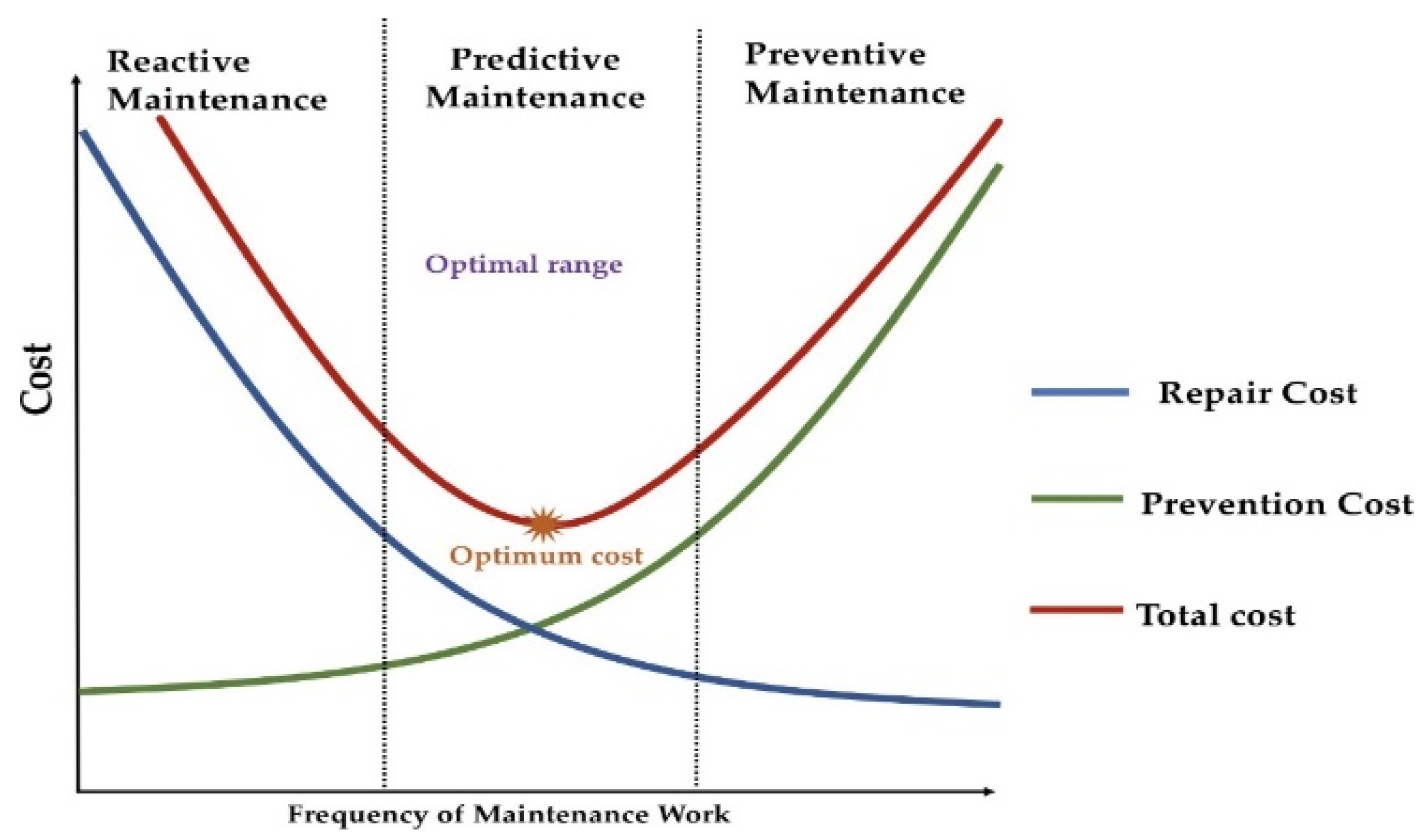
31], using a predictive strategy rather than depending only on scheduled preventive maintenance may result in potential energy savings of around 8-12%. The use of predictive maintenance strategies has been shown to have a positive impact on the longevity of assets, as well as a reduction in equipment downtime and associated expenses related to replacement parts and labour as shown in
Figure 1. Furthermore, this methodology enhances worker safety, enhances plant dependability, and optimizes the functioning of the equipment, resulting in immediate energy savings. However, this particular strategy necessitates an initial investment in cash for the procurement and installation of diagnostic equipment [
32,
33]. Furthermore, the successful implementation of the company's selected predictive maintenance system necessitates a substantial investment in staff training. In a general sense, the benefits of this strategy are greater in magnitude than the drawbacks. According to surveys conducted on the industry average savings, it was seen that enterprises had a significant improvement in their operational efficiency after adopting a predictive maintenance program. Specifically, these companies reported a reduction of around 70-75% in asset breakdown, a decrease in maintenance expenses by 25-30%, and an increase in output by 20-25%. The average return on investment (ROI) was 10 times, indicating a favourable investment.
2.6. Finite Element
The Finite Element Method (FEM) is a numerical technique for solving problems in engineering and physics [
34]. It approximates the solution to a partial differential equation (PDE) over a complex domain by breaking it into many smaller, simpler elements. The method is widely used to analyse structures, fluids, and other physical systems. FEM is based on breaking down the problem domain into many smaller elements, each of which is assumed to have a simple, known solution. The solution for the entire domain is then obtained by solving for the unknowns at the nodes where the elements meet [
35]. The FEM is widely used in mechanical engineering, aerospace engineering, civil engineering, biomedical engineering, and many more, as it can handle complex geometries, loading conditions, and material properties. High Cycle Fatigue (HCF) is well-known and researched for fatigue testing. However, the testing was done with constant loads. The fatigue life for helical springs was examined based on the critical constant loading. Reference [
36] evaluated the multiaxial strength coiled springs used in suspension systems by applying Von Mises and critical plane criteria through the investigation of the HCF life using start-stop conditions aligned with the analysis of fractured surfaces using failure analysis. Reference [
37] performed the same research as reference [
38], despite the similarities between their results’ outcomes, both results gave the exact estimation of the fatigue calculation. [
39] did not just examine the fatigue strength with the HCF; however, he did combine the impact of the axial and torsional loading on the fatigue strength. Reference [
40] examined the stress distribution and all the parameters that impact the stress distribution.
2.7. Fatigue Analysis
Fatigue is the leading cause of the failure of the coiled springs as shown in
Table 1; however, many factors impact the fatigue life, such as surface roughness, material decarburization, and material defects like inclusions. The cold coiling method of manufacturing coiled springs causes residual stress distribution, impacting fatigue life [
41,
42]. It is evident in reference [
42] that the fatigue limit of the helical springs depends on the residual stress field through experimental investigation. The traditional methods to estimate fatigue life cycles for mechanical coiled springs are based on fatigue strength with torsion [
41]. Modal analysis is a computational method that studies the dynamic properties of suspension systems in the frequency domain. The modal analysis ignores the forces acting on the coil spring; however, it depends on its mass and stiffness.
2.8. Novelty of this Paper
Fatigue analysis is based on current real-time data that considers the impact of specific factors that cause systems’ deterioration throughout a given period.
Digital Twin (DT) method is used to improve systems’ empirical predetermined loads and lifecycles.
Entire mechanical behaviours of systems are visualized continuously in real-time.
3. Methodology
Three different tests are used in this paper. First is an experiment fatigue analysis done in the lab, the second is a Finite Element analysis of the same spring for fatigue analysis, and finally the third test is the Digital Twin test for fatigue analysis. The first two tests are used to be compared against the third method for validation, comparison with the existing literature is also done.
3.1. Materials
The materials used to develop the coiled spring used in the suspension system were calculated using the empirical formula—the empirical formula based on the maximum tensile strength of the materials used in the development.
3.2. Experimental Method
This section describes the practical investigation conducted based on experimental testing for fatigue analysis. Two experimental tests are available to analyse fatigue and predict the systems' life cycle [
39,
50,
51]; One is the constant amplitude test (fixed forced), and the other is the programmed test. In this study, the programmed test was used; the empirical testing is based on the block cycle loading, where the coiled spring rate, strain, and stress are measured. The experiment used in this paper aimed to analyse the suspension system’s fatigue life, determine the system’s lifecycle, and compare the results with the DTM.
3.2.1. Theory
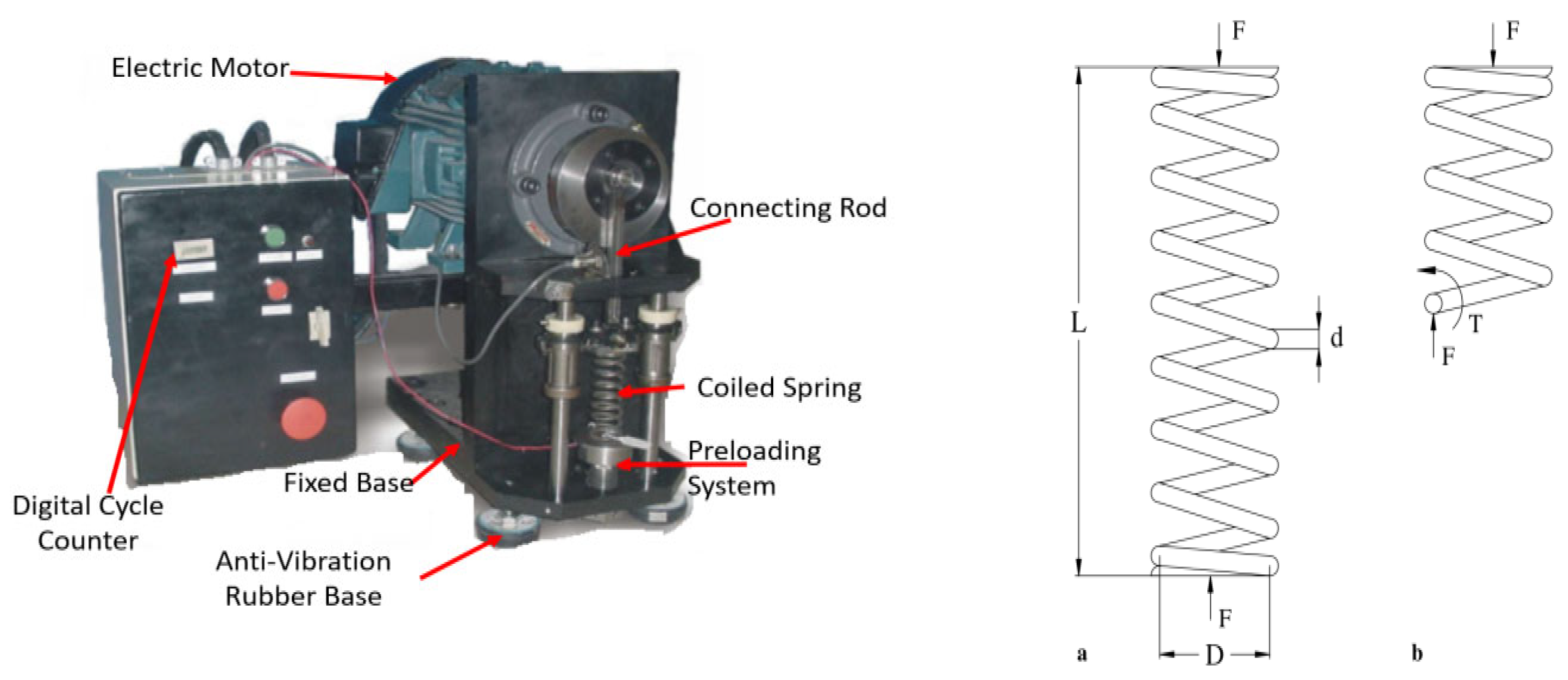
As shown in
Figure 2(a) the helical spring is exposed to an axial load denoted as F. In order to ascertain the stress induced in the spring. Consider the scenario where the spring is divided into four sections or four groups representing the four springs used in a suspension system in an automotive vehicle at a certain location, as seen in
Figure 2(b). These four springs or four groups are treated with heat. The heat treatment was conducted on an electrical furnace with automatic temperature control as follows or divided into groups as follows: Group (1) heated at 200 C
o for 10 minutes, Group (2) heated at 300 C
o for 15 minutes, Group (3) heated at 400 C
o for 20 minutes, Group (4) heated at 500 C
o for 25 minutes.
Internal forces are produced in order to establish and sustain equilibrium inside the remaining section, as seen in
Figure 3(b). A direct shear force, denoted as F, and a torque, denoted as T, are present. The maximum shear stress on the wire can be determined using the following equation.
Equation (1) represents the maximum shear stress τmax in a material subjected to torsion and axial loading where:
± represents the sign of the shear stress, which can be either positive or negative.
T is the applied torque.
r is the radius of the shaft.
J is the polar moment of inertia of the shaft cross-section.
F is the axial force applied to the shaft.
A is the cross-sectional area of the shaft.
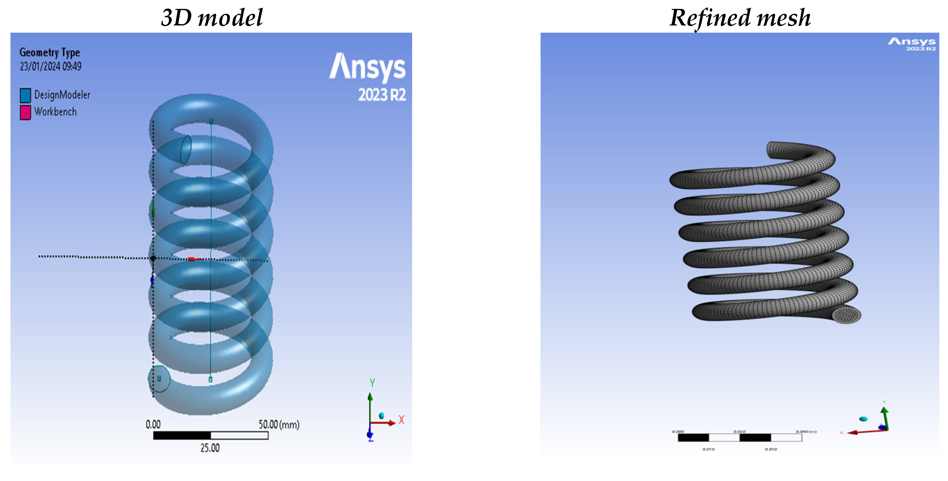
Figure 3.
Shows The A- Initial 3D Model, B- Mesh Applied to the 3D Model.
Figure 3.
Shows The A- Initial 3D Model, B- Mesh Applied to the 3D Model.
The equation is important in mechanical engineering as it helps in determining the maximum shear stress in a material subjected to torsion and axial loading. This information is crucial in designing and analysing various mechanical components such as shafts, gears, and springs, and in this project is used for the spring.
Where D is the mean coil diameter, K is the Wahl factor, C is the spring index defined by
When the external force F, is in a transient mod, the induced stress is the variable as well. Therefore, the mean stress
and the amplitude
are defined by:
Where Ks and Kb are the correction factors due to curvature and Fm and Fa are the mean load and the load amplitude, respectively.
3.2.2. Relaxation and Fatigue Tests Experiment Description
The objective of the relaxation test is to examine the change in the spring constant subsequent to a sequence of load cycles. The fatigue testing equipment seen in
Figure 2 comprised springs that were exposed to a cyclic load. The spring constant, denoted as
, which represents the ratio between the force exerted, F, and the resulting deflection of the spring, d. In this study, a series of relaxation tests were performed to quantify the force, denoted as F, required to induce a deflection of 20 mm. The fatigue testing equipment was configured with preload and load amplitude values of 30 mm displacement and 25 mm, respectively. The spring constant was determined after doing 50,000 cycles. The primary aim of the experiment was to find the fatigue life cycles and to analyze the impact of cyclic loading in an ambient setting on spring relaxation, with a specific focus on the changes in the spring constant.
A fatigue testing apparatus has been developed with the purpose of determining the S-N curve for helical compression springs as seen in
Figure 2. The mechanism facilitates the application of force in alignment with the axis of the spring. The specialized equipment designed specifically for this purpose was used to conduct these tests. The fatigue testing equipment is seen in
Figure 2 use of a slider-crank mechanism facilitates the conversion of rotational motion from a motor into rectilinear alternating motion, ultimately resulting in the application of cyclic strain to the spring being tested. The machine is equipped with a 7.5 HP electric motor that generates the required driving power to induce deformation in the active coils of the spring at a frequency of 25 Hz. In the event of a spring failure, the fatigue testing equipment ceases operation immediately, while a digital cycle counter records the fatigue life of the spring. The experiment included conducting fatigue tests with a constant mean stress,
of 300 MPa, while varying the stress amplitude,
. In order to do this, the preload and amplitude displacement of the connecting rod were modified for each test, resulting in the attainment of the required values of
and
as outlined in Equations (4) and (5). At this stage, the testing time will be so long and need a significant reduction; one way to accelerate the testing time is to preload the spring with a specific force. In this case, the spring was preloaded with three different loads (0.7, 0.8, and 1) KN, respectively, with an average of 0.8 KN. The potential damage resulting from the accelerated testing was the same as the one done in actual fatigue testing; based on the regular practice for accelerated testing, the conditions of preloading and the frequency of loading is 25 Hz used when choosing the block load cycles, which resulted in testing the spring for 9*10^6 cycles (12.2 hours =12 h and 12 minutes).
3.3. Computational Method
The prediction of the fatigue lifecycle is usually carried out using three different approaches. The first approach is the linear elastic fracture, the second is the stress life approach, and the third is the local strain life. In this paper, Ansys software is used to analyse fatigue lifecycles. The strain life approach is also elected because its suitability for the load sequence and mean stress impact is essential for fatigue analysis [
48].
3.3.1. Strain Life Approach
The use of the local strain-life technique is warranted in situations where the loading history is characterized by randomness, and where the influence of mean stress and load sequence effects is deemed significant. The methodology used in this study encompasses many methodologies aimed at transforming the loading history, geometry, and material properties (both monotonic and cyclic) into a position of fatigue life. Initially, the stress and strain inside the crucial zone are evaluated, followed by the use of the Rainflow cycle counting approach to minimize the load-time history. The subsequent procedure involves using the finite element technique to transform the diminished load-time history into a strain-time history, as well as determining the stress and strain within the region experiencing significant stress. Subsequently, the fracture initiation procedures are used for the purpose of forecasting the fatigue life. The accumulation of fatigue damage is facilitated by the use of the simple linear theory, as presented by Palmgren and Miner. Ultimately, the cumulative damage values of each cycle are aggregated until a predetermined threshold of critical damage is attained, which serves as the failure criterion. This research used the strain life analysis methodology to determine the fatigue life. The characterization of the fatigue resistance of metals may be accomplished via the use of a strain-life curve. The mathematical expression of the link between the total strain amplitude
and the number of reversals to failure (2N
f) is given by the Coffin Manson (CM) Model as shown in Equation 6.
Where the meaning of each term is shown in
Table 2.
The absolute maximum principal strain method is used to combine component strains
Where
εAMP is the absolute maximum principal strain, and
ε1 and
ε3 are the principal strain The Morrow (Mo) model is used for stress (
σm) corrections:
The Smith Watson Topper (SWT) strain life model is mathematically expressed by Equation 9.
The three strain-life expressions involve various parameters. E represents the material modulus elasticity, σmax denotes the true maximum stress, σm represents the mean stress, εa signifies the true strain amplitude, 2 Nf corresponds to the number of reversals to failure, σf' denotes the fatigue strength coefficient, b represents the fatigue strength exponent, εf' signifies the fatigue ductility coefficient, and c represents the fatigue ductility exponent.
3.3.2. 3D Modelling
The dimensions specified in
Table 2 are used to model the coil spring in CREO and the hardware components used in this study are shown in
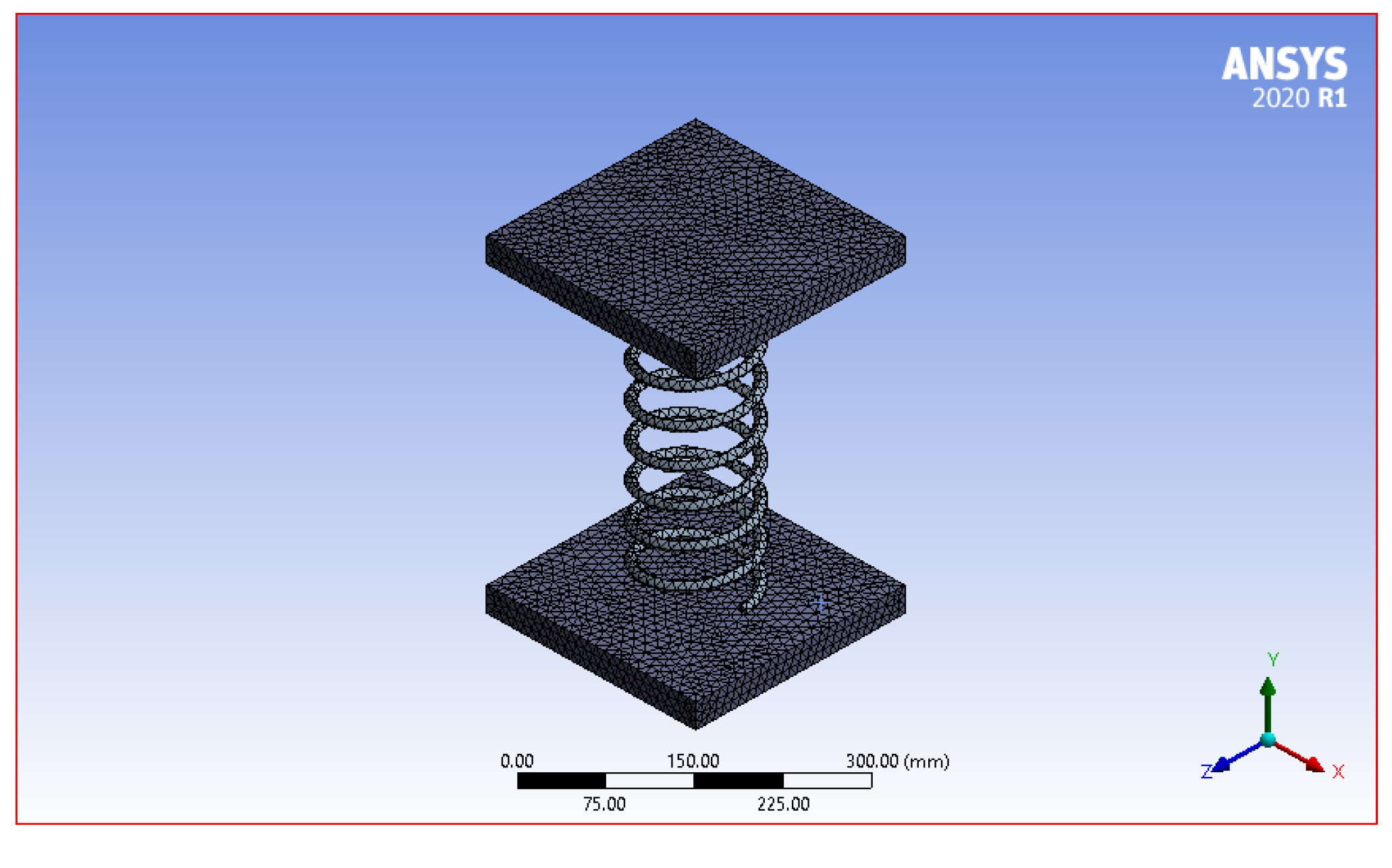
Table 3. The sketcher used to draw both the wire and mean diameter. Setting the helix option allows the entries for the total number of coils, active coils, constant pitch, and choosing clock or anti-clockwise for the specified—sweep option selected to visualize the 3D model of the system entirely. The parameters used in this design are the exact parameters for the coiled spring used in Peugeot 3008. The part was imported into ANSYS Work Bench (WB) 2020 R1 using the format of IGES. Tetrahedron 10 and 20 elements mesh applied to the coil spring. Refining the mesh ensures the accuracy of the fatigue analysis; the mesh is refined with the material properties shown in
Figure 2.
3.3.3. Boundary Conditions
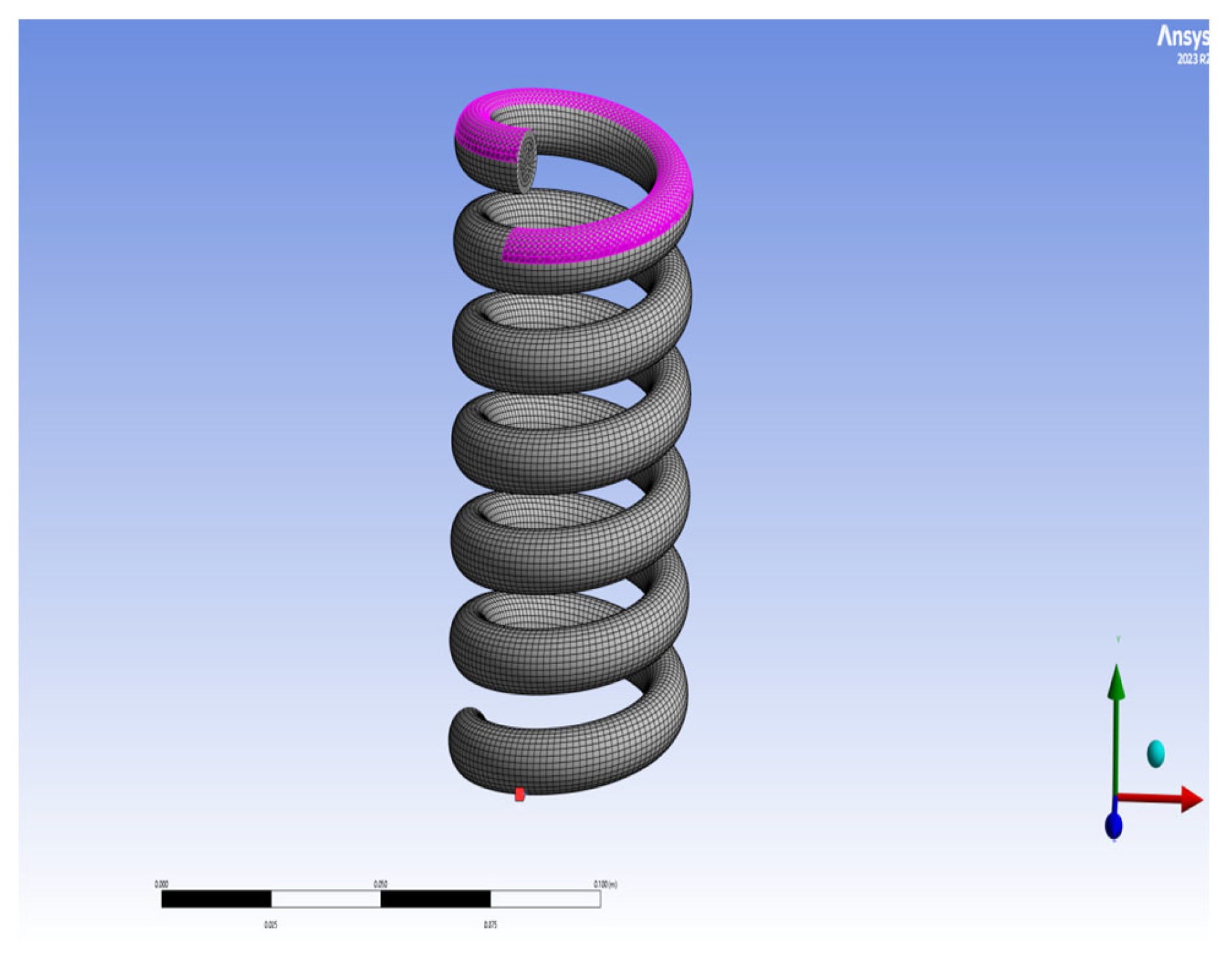
ANSYS software was used to analyse the mechanical behaviours of the coil spring created as parts modelled in CREO. Since this analysis is static, using ANSYS modelling, apply the boundary conditions, and
Figure 4 shows the boundary conditions applied on the upper ring of the coil spring while the lower part is treated as a fixed end.
Engineers struggle to find a reliable balance between cost and accuracy (CPU time); however, performing mesh sensitivity analysis on the model ensures the balance required as shown in
Figure 5.
3.4. Digital Twin Method
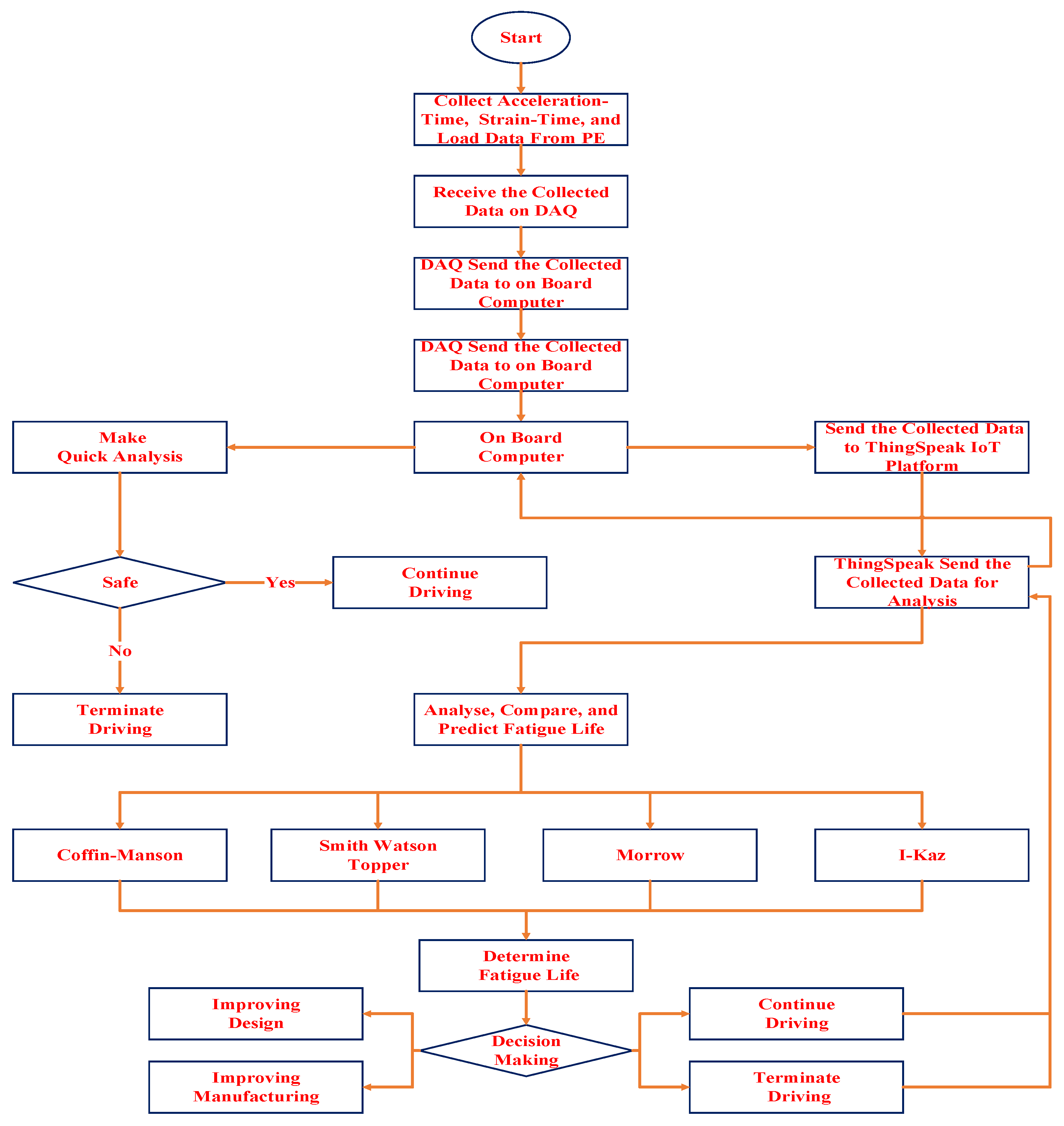
The DT method used in this research includes five primary stages: (1) Current Real-Time data collection, (2) IoT platform (ThingSpeak) for data aggregation (3) Signal processing, (4) Finite Element Analysis (FEA) of the coil spring, and (5) Decision Making.
Figure 6 depicts the flow chart illustrating the methods used in this investigation.
This paper proposes four dimensions DT concept namely (Physical Entity (PE), Virtual Entity (VE), Connection between VE and PE, Time) with high accuracy and efficiency as shown in
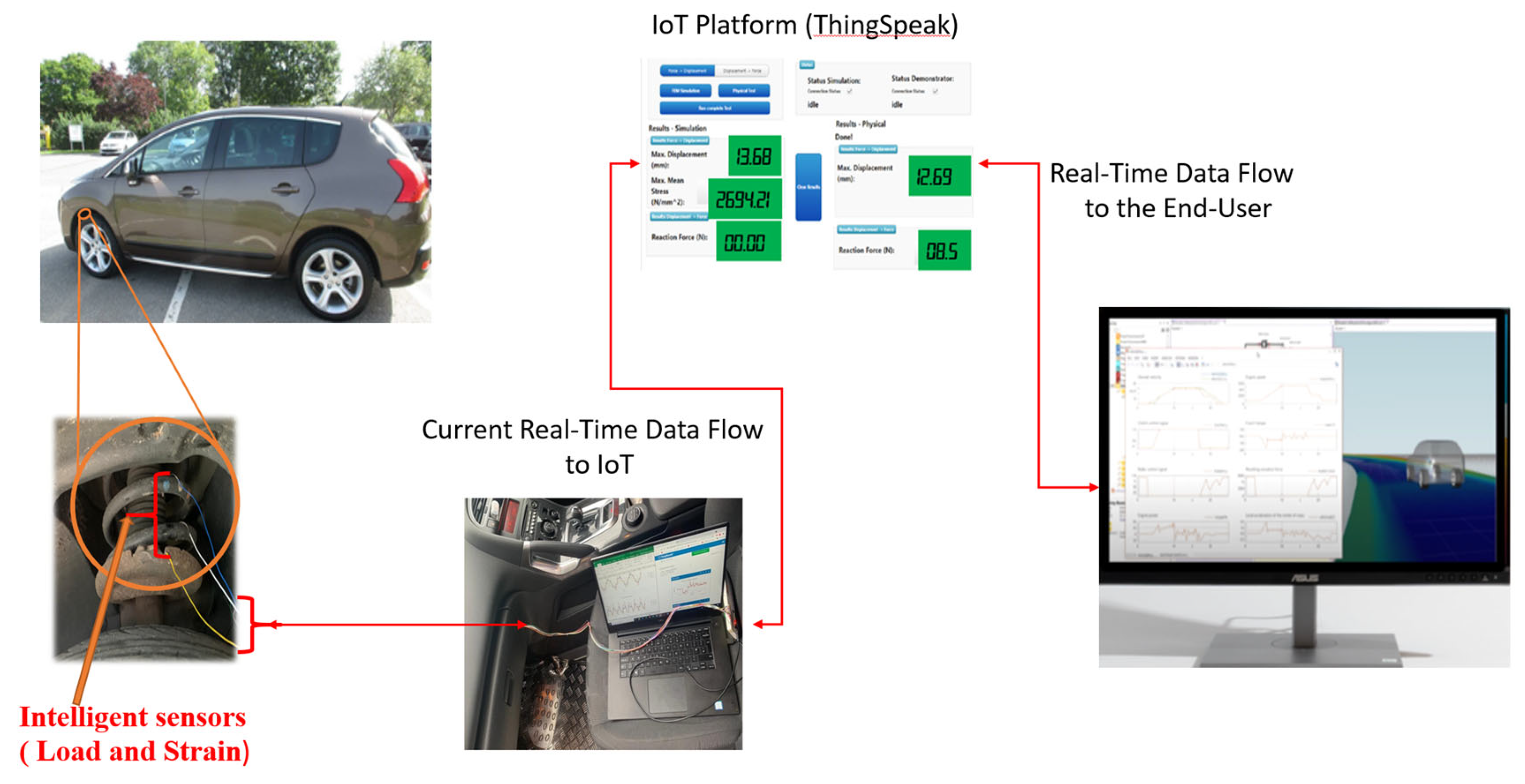
Figure 6. The concept is validated through fatigue analysis and comparison with the latest literature methods of a coiled spring used in suspension systems in the automotive industry. Additionally, this concept is not limited to the automotive industry but is applicable to any industry keeping the different parameters for different applications into consideration; with the same four dimensions mentioned. The proposed concept reports continuous current real-time mechanical behaviours (force, displacement, stresses, and strains) acting on the system using intelligent sensors, as shown in
Figure 7. Sensors collect current real-time data with any mechanical behaviour changes within the system; the Data is received by the ThingSpeak Internet of Things (IoT) platform, where the data are analysed and aggregated, then sent to software (MATLAB / ANSYS) to trigger a live simulation.
3.4.1. Hardware and Data Collection
For the purposes of this research, a 2000 cc Peugeot 3008 car was selected as the vehicle for the case study. As shown in
Figure 7 the car type under consideration is equipped with a front MacPherson strut suspension system, a widely used configuration across several vehicle models. A uniaxial accelerometer was affixed to the lower control arm of the vehicle in proximity to the hub carrier, while a strain gauge was affixed to the coil spring. The location at which the strain gauge was affixed corresponds to the point of maximum stress, as estimated using Finite Element Analysis (FEA).
Figure 7 depicts the schematic design of the experimental configuration. To ensure the stability of the sensors during data collection, a robust glue was used to connect both the accelerometer and strain gauge to the designated measurement locations. The strain gauge used in the experiment had specified characteristics of a gauge length of 2 mm, a gauge factor of 2.07 ± 1.0%, and a resistance of 120 X. The accelerometer employed was of the piezoelectric type, with a sensitivity of 1.02 mV/(m/s2), a measurement range of ±4900 m/s2, and a frequency range spanning from 0.5 to 10 kHz. The data collection system was used to establish a connection between the accelerometer and strain gauge. This system captured the signals received by these sensors, which were then communicated to a laptop computer. Following this, the strain-time and acceleration-time histories were seen in real-time on the laptop computer and sent at the same time to the ThingSpeak IoT platform as shown in
Figure 7.
3.4.2. ThingSpeak IoT platform for Data Aggregation
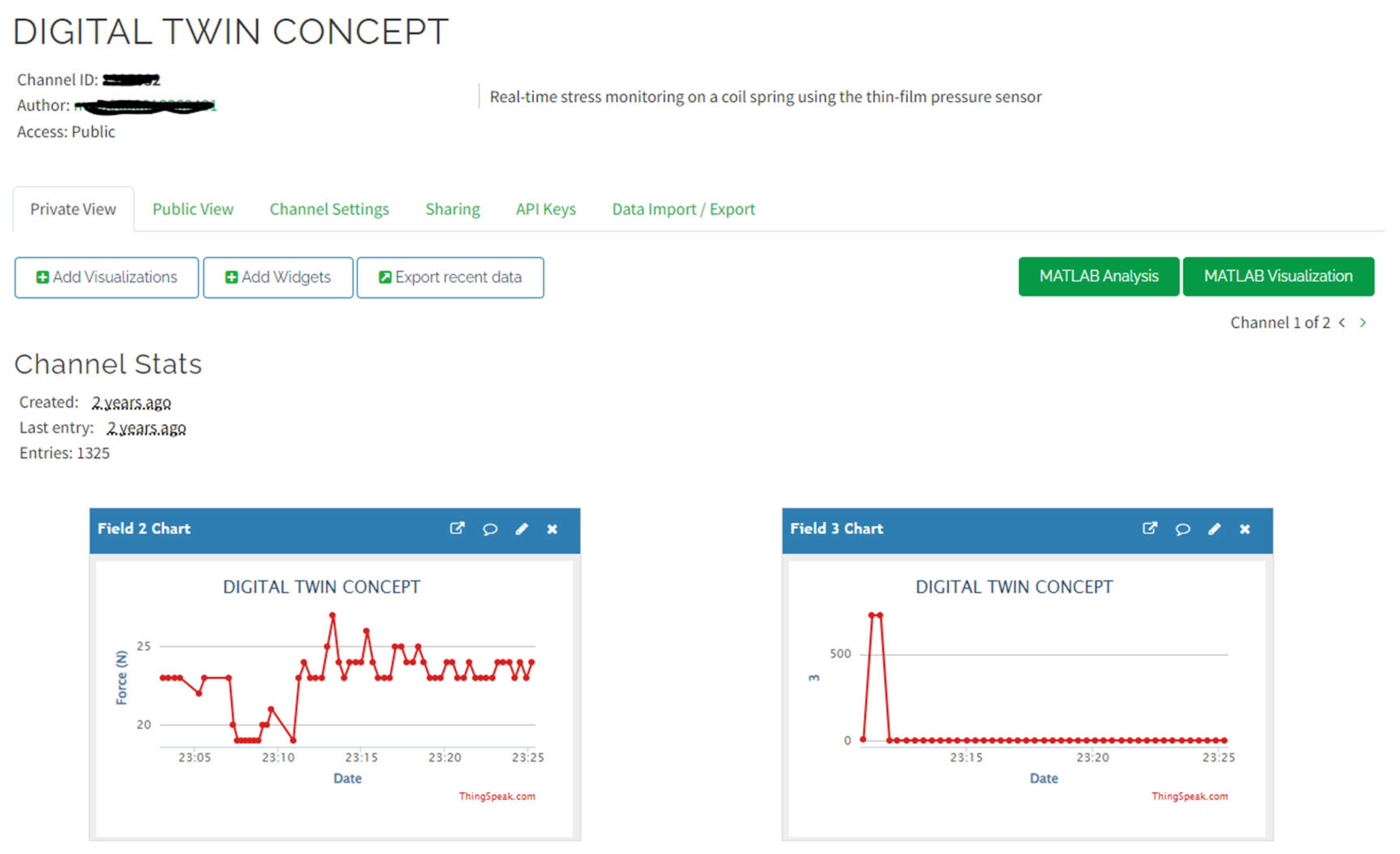
The second stage is developing the IoT platform. In this study, the ThingSpeak IoT platform is selected for its simplicity, cost-effectiveness, capabilities, and integration with MATLAB analysis. ThingSpeak is an Internet of Things (IoT) platform that facilitates the collection, visualization, analysis, and response to current real-time data. The open-source program was first released in 2010 by ioBridge. It facilitates the development of Internet of Things (IoT) systems without the need to establish additional servers. Access to the ThingSpeak IoT is available from any browser. A dashboard was created to control, aggregate data, and connect the DTM and the PE. Public and private channels built under specific IDs write and Read API keys. Each channel has up to 8 fields, representing input from one sensor, as shown in
Figure 8. The process of data collecting is facilitated by the use of REST API or MQTT as shown in
Figure 7. The process of data analysis and visualization is conducted via MATLAB analytics. Additionally, users have the ability to include numerous plugins that allow for the inclusion of Google Gauge and other customized visualizations and controls inside a private viewing setting. The primary component of ThingSpeak is its channel, which serves as a repository for data sent from diverse devices. Each channel has the capability to store a maximum of eight fields, including device location, URL, and other relevant information. The channel has the option to be either public, visible to other users, or private, requiring an API key for data access. The private channel has the capability to be shared with a select group of users as shown in
Figure 8. The communication mechanism used is based on the publish-subscribe paradigm. The entity responsible for generating and disseminating information is often referred to as the publisher. The individual or entity that expresses interest in obtaining the disseminated information is often referred to as the subscriber.
3.4.3. Signal Acquisition
In this study, signal filtering was not conducted since the fatigue process relied on the peak and valley of the strain signals, with even minor amplitudes contributing to the fatigue calculations. The use of strain time history filtering has been shown to result in a reduction in computing time. However, it is important to note that this approach may provide major challenges in accurately predicting fatigue damage, as highlighted in previous research. As stated by Ilic (2020), it is recommended that the sampling frequency for the load signals exceed 400 Hz. However, the typical frequency range used for the measurement of vibration fatigue is between 10 and 1000 Hz. Therefore, a sample frequency of 800 Hz was used in order to adequately capture the reactions generated by the road profiles across all frequencies. The fatigue study of automobile coil springs under time-varying loads becomes inherently difficult when a vehicle traverses a rough road, since the stresses experienced are both random and non-stationary. The majority of existing fatigue algorithms in the time domain rely on cycle-counting approaches and damage accumulation criteria [
48,
52,
53]. In order to replicate a random process, it is necessary to use numerous time histories. Due to this rationale, it is necessary to use diverse road profiles to accurately anticipate the fatigue lifespan and assess the design of car coil springs. Subsequently, the Peugeot 3008 is operated on a variety of road types, including highway, residential, rural, hill, and mixed with the purpose of gathering random vibration data as shown in
Figure 9.
The highway road profile exhibited a more uniform road surface, leading to the anticipation of achieving a vehicle speed of 70 m/h. The rural road profile exhibited an irregular and coarse texture, with the anticipation of encountering some areas of pavement deterioration in the form of potholes. The residential road exhibited a notable presence of speed bumps, leading to anticipation of elevated levels of vibration responses from vehicles traversing the road. The average speed of vehicles on rural and residential road profiles was around 25 m/h as a result of these constraints. The profiles of the hill and mixed roads exhibit a notable presence of bends and curves, so introducing supplementary stresses on the automotive coil spring of the front MacPherson strut suspension system. The velocity of the vehicle was around 50 m/h for the hill and mixed road profiles. Notwithstanding the fluctuations in vehicle velocity, the models included authentic vehicle vibrations generated by road stimuli, using the corresponding data.
4. Experimental Method Results
4.1. Relaxation Test
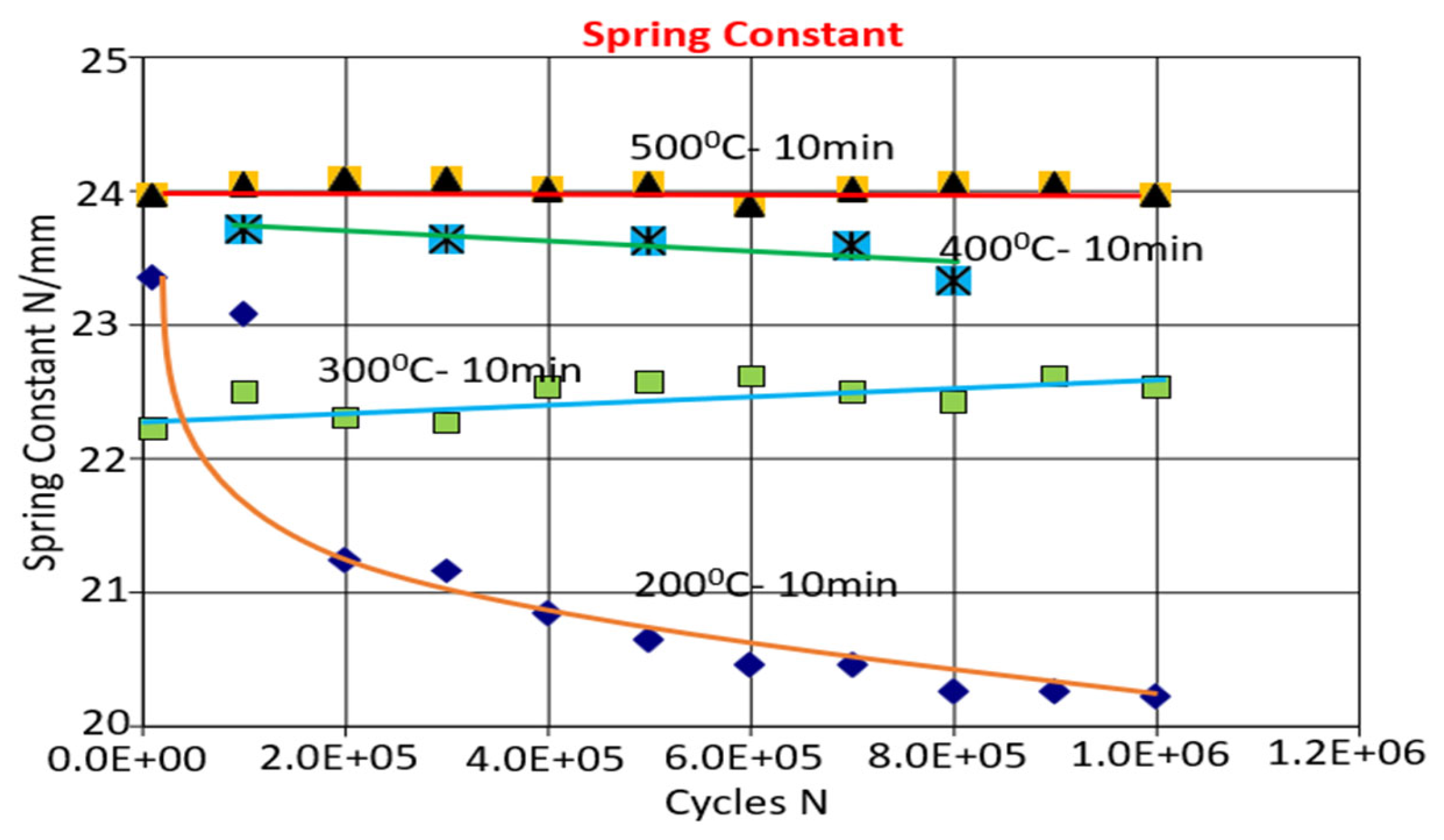
The relaxation test results are shown in
Figure 10. The diagram illustrates the relationship between the spring constant, denoted as k, and the number of load cycles. It should be noted that the parameter k remains constant under cyclic loading conditions, with the exception of the 200°C for 5 minutes group, where a gradual reduction in k is noticed. However, after 700,000 cycles, a stable value of k is achieved. In order to enhance the performance of a spring during the spring season, it is crucial to understand the impact of heat treatment on the coefficient of spring stiffness (k value). The behaviour shown by the group subjected to a temperature of 200°C for a duration of 10 minutes may be elucidated by considering the occurrence of a relaxation phenomenon inside the material as a result of cyclic loading. The observed phenomenon may be likened to cyclic softening, when the stress decreases as the number of cycles increases. This behaviour has been shown in some materials during cyclic plasticity testing, namely in the case of SAE steel as documented in reference [
35].
4.2. Fatigue test
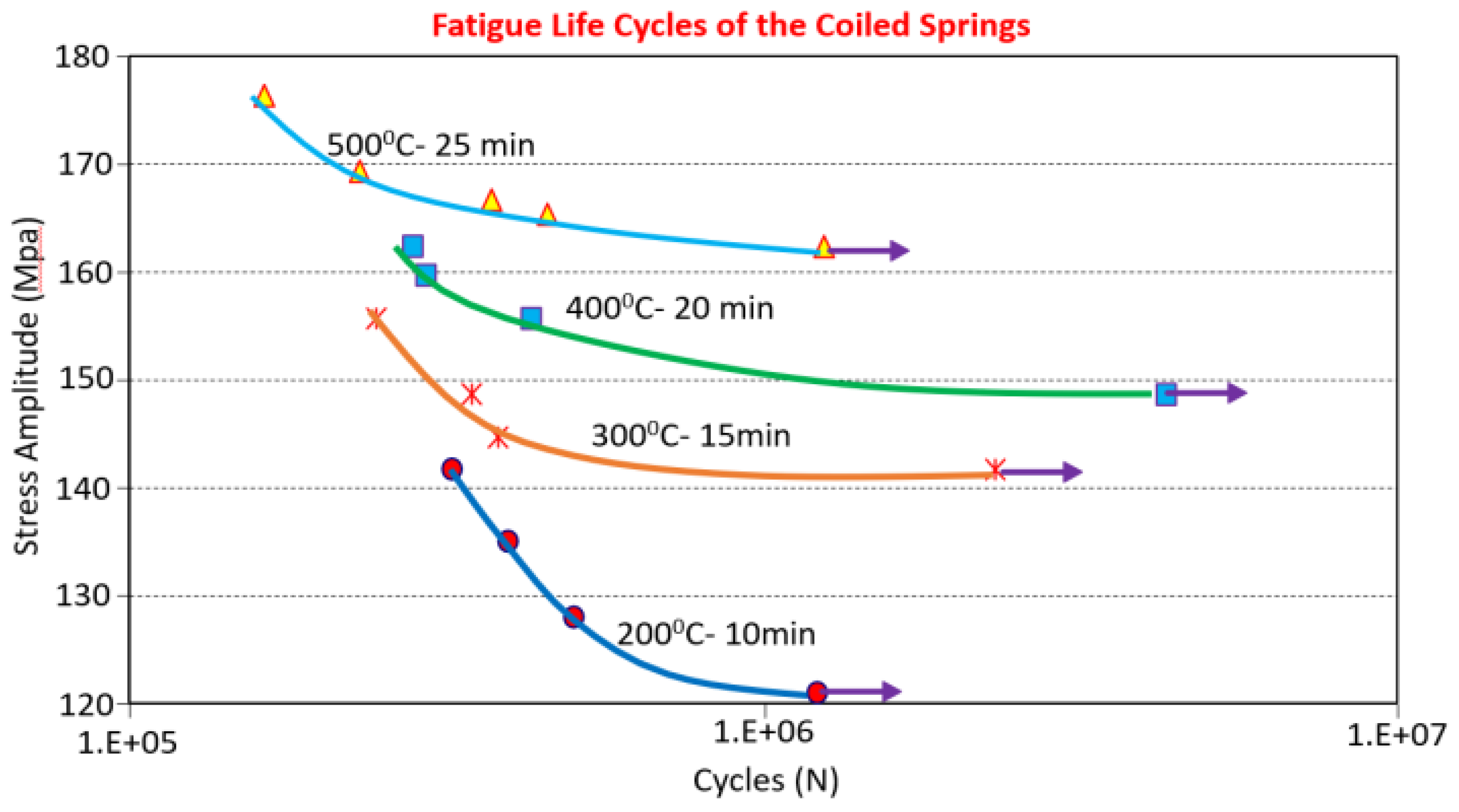
The fatigue curves are established for each spring or for each group of springs. The findings are shown in
Figure 11, whereby the arrows inside the plot indicate instances when the test was terminated prior to the occurrence of spring failure. As shown in the provided figure, it can be seen that the group exhibiting the highest fatigue limit
was subjected to a temperature of 500°C for a duration of 25 minutes, resulting in an estimated value of
= 160 MPa. The experimental condition characterised by a temperature of 200°C and a duration of 10 minutes had the lowest fatigue limit, measured at 120 MPa. Furthermore, this condition demonstrated the most variability in the spring constant, as seen during the relaxation tests. The experimental condition with a temperature of 400°C and a duration of 20 minutes exhibited an intermediate fatigue limit, denoted as
, with a value of 148 MPa. In a similar vein, the experimental group subjected to a temperature of 300°C for a duration of 15 minutes exhibited a fatigue limit of 140 MPa.
Since no cracks were noticeable on the spring and the resultant spring stiffness was nearly the same; therefore, the spring sustained 8.9*10^6 cycles during the accelerated block load cycle test without any failure as shown in
Table 4.
5. Computational Method Results
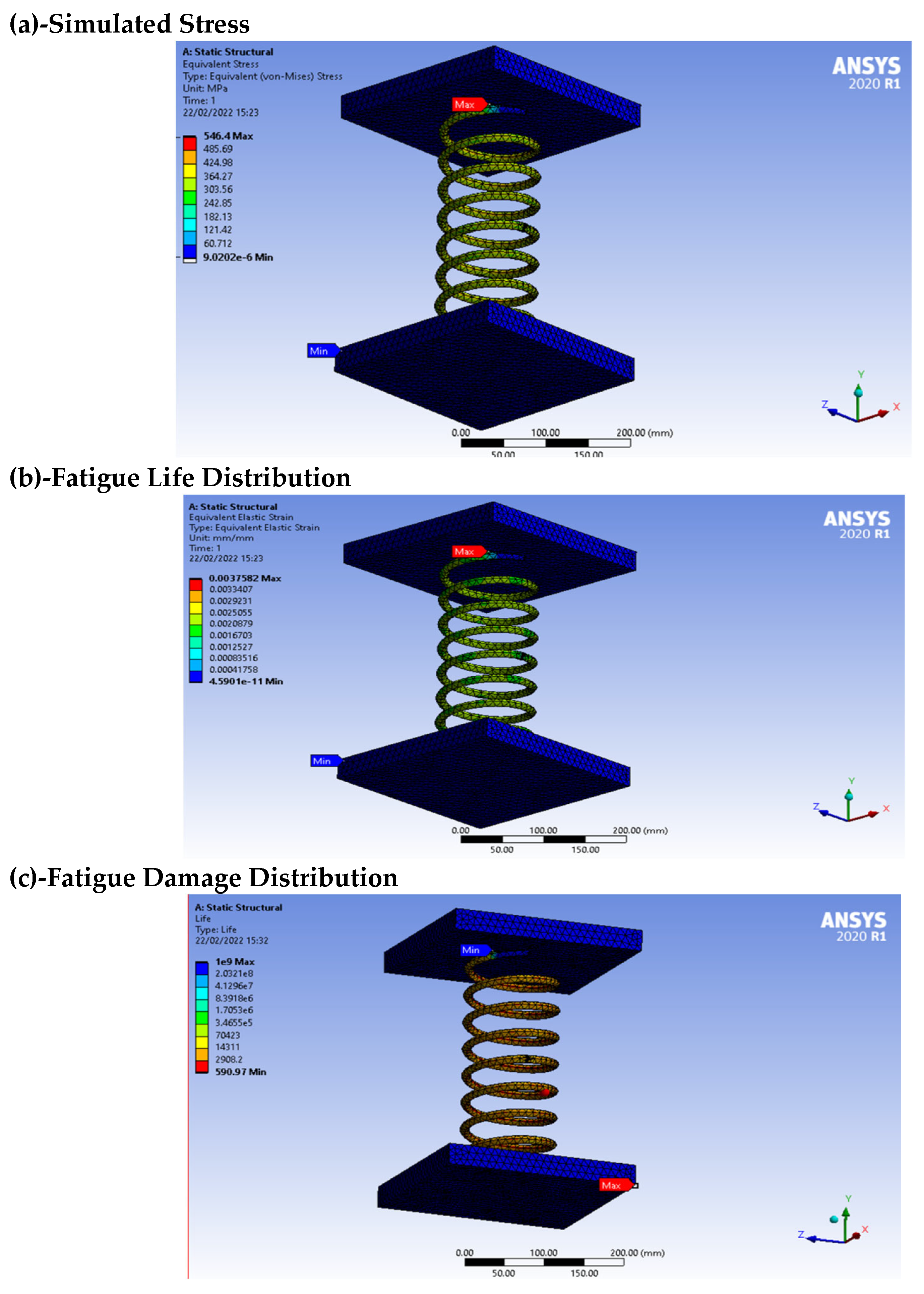
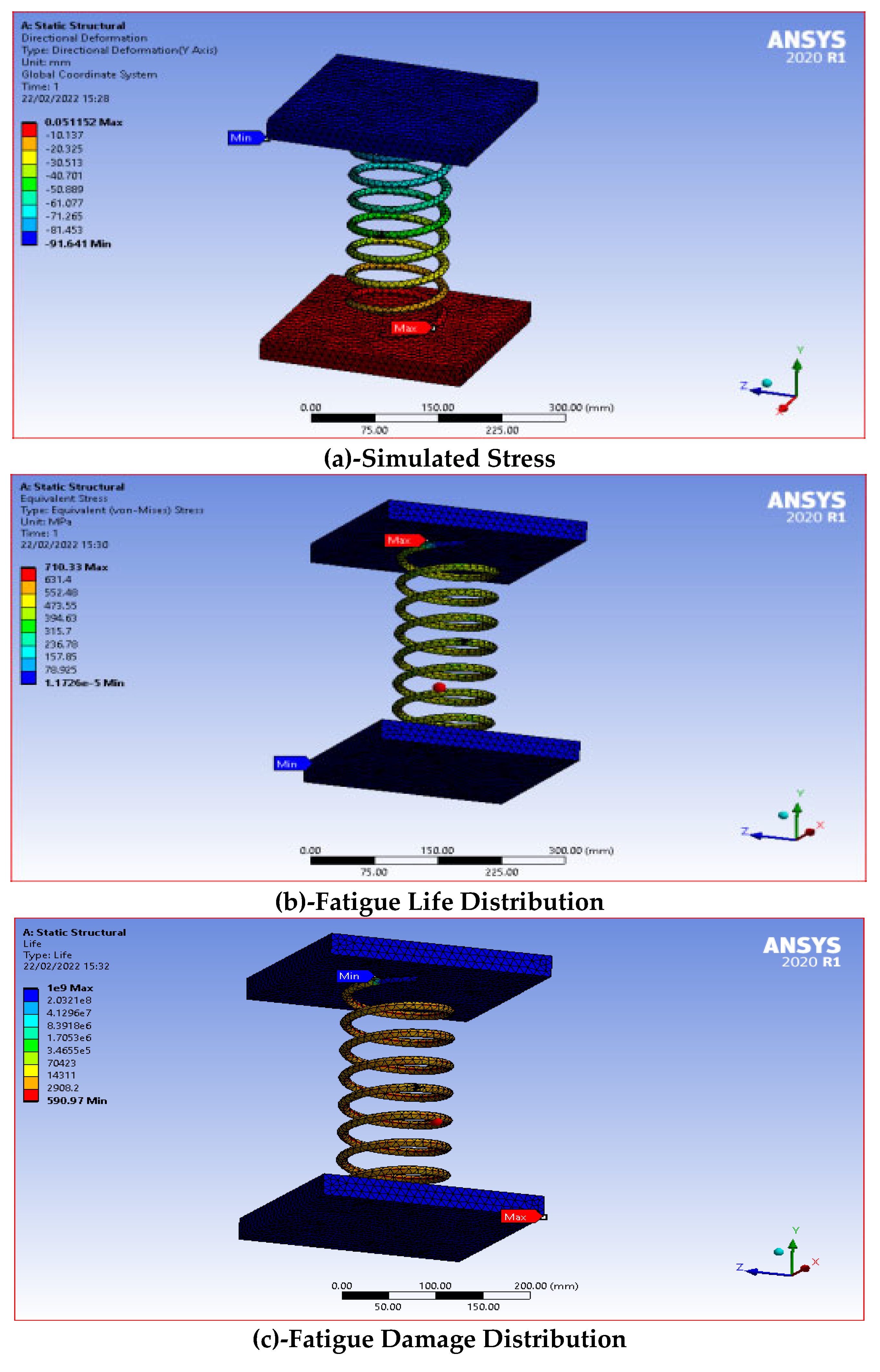
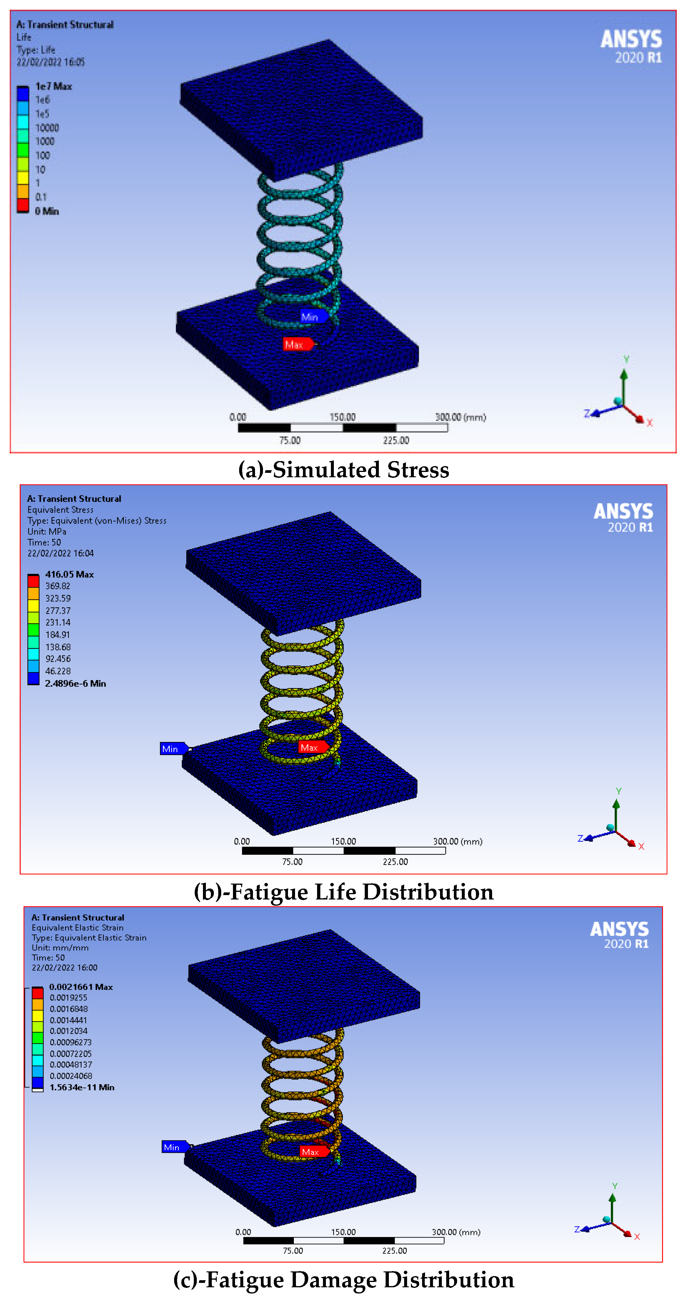
The examination of fatigue is mostly centred on the outcomes obtained at the key area and its surrounding vicinity, as seen in
Figure 12. The selection of this location is based on the experimental findings presented by [
50], which demonstrate that fatigue failure in coil springs occurs mostly in the active coils located distant from the inactive coil that serves as the spring's seat. Contours in
Figure 12 (b) and (c) depict the representation of life and reported damage. It is evident that the spring will not experience fatigue failure throughout its designated lifespan of 4×10⁵ cycles at the key site, as shown by both time histories [
35]. The figures denoted as
Figure 12,
Figure 13 and
Figure 14 show the highest recorded levels of damage, as indicated by circular markers. The observed phenomenon may be attributed to a geometric modelling discontinuity resulting from the variable pitch of the coil. Abrupt changes in the orientation of the coil result in an elevated area of mechanical strain. Due to the considerable distance between these sites and the crucial area, their impact on the findings provided at the key site is deemed insignificant, hence warranting their exclusion from the fatigue study.
Figure 12 shows sudden changes in the stresses throughout the spring from top to middle; however, the top result is likely obtained from the surface contact definition with the spring. In order to take into consideration, the effects of mean stress during the process of estimating fatigue life, researchers have turned to not one but two separate models: The Morrows model and the Smith Watson Topper model (SWT). The life estimate plot that was derived by using the SWT model can be found in
Figure 5. In environments with the highest levels of stress, the average number of life cycles of the coil spring is around 4.24*10^6. Using Morrow's model, we were able to calculate the predicted fatigue life Smith Watson Topper model 5*10^5.
It is essential to show the critical location for the fatigue analysis because it will focus on the critical places and their area. In the experimental work of [
41], selected critical locations that impacted the failure of the spring in the active coils, which were far from the inactive coils;
Figure 13 and
Figure 14 show that might be the exact scenario. Additionally, reference [
41] leads from experimental work of the spring will not fail at the critical location; therefore, in this case, the system withstands its design life cycles of 3.6*10^6.
Figure 12,
Figure 13 and
Figure 14 show the maximum damage at the critical locations marked with red circles is likely because of the change of directions of the coil, as shown in
Table 5 and these are the areas where the modelling discontinuity occurs; therefore, the critical locations marked with red circles experience the highest stress across the spring. The observed locations are marked with red circles far from the critical regions used for fatigue analysis.
6. Digital Twin Method Results
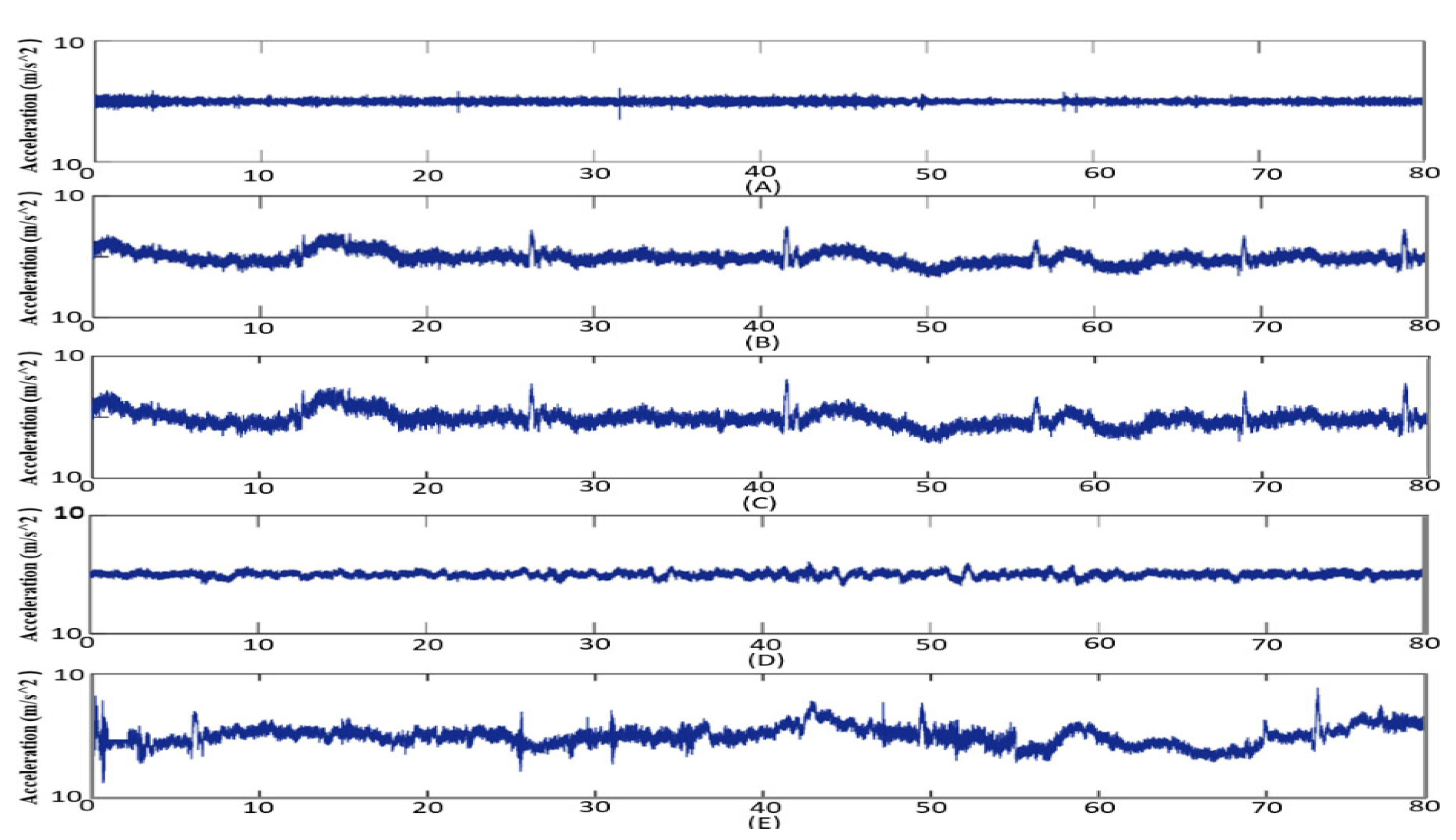
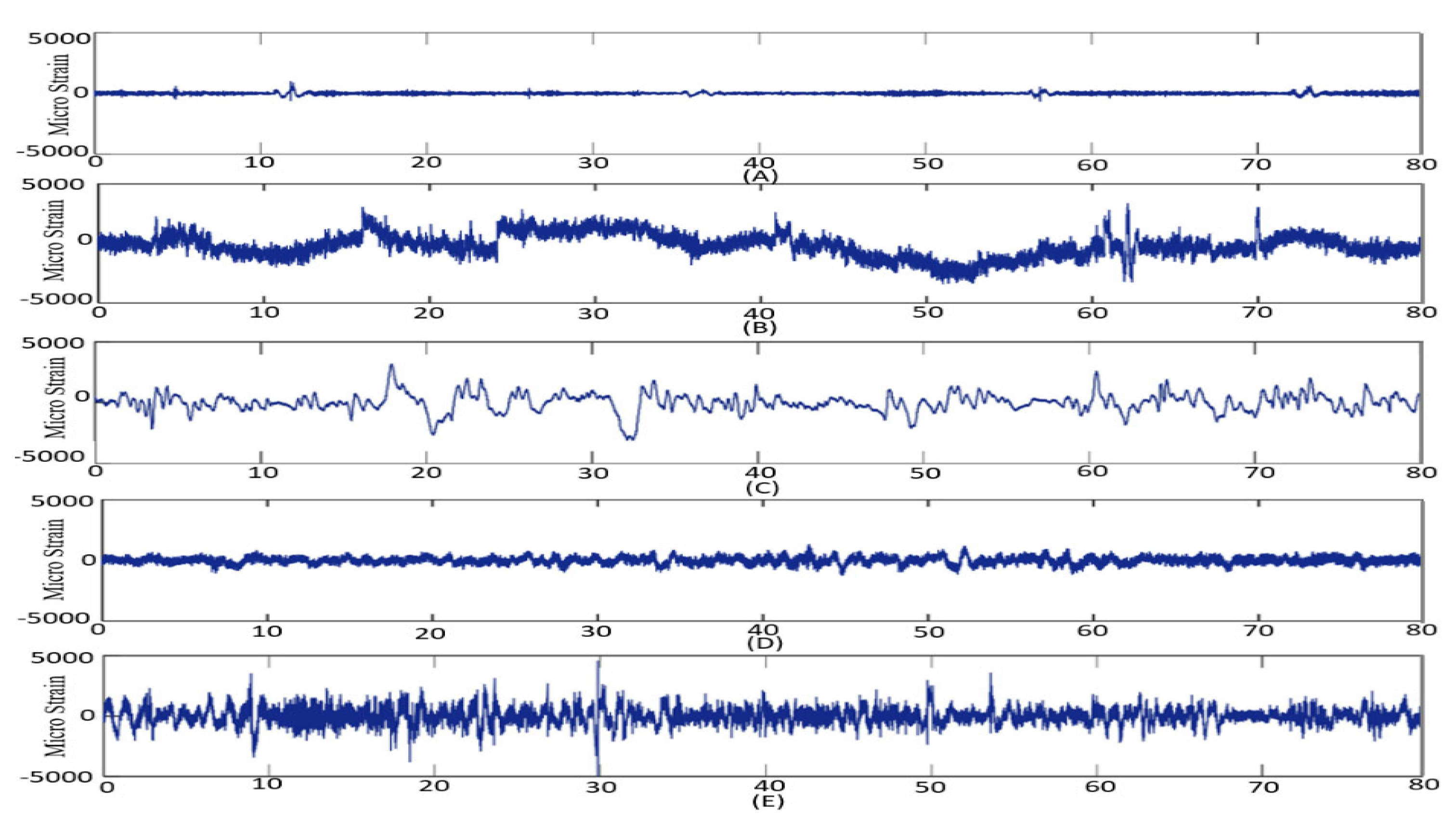
Figure 15 and
Figure 16 from A to E, the acceleration-time histories and macrostrain-time histories for five road profiles were obtained. A comprehensive set of 64,000 data points was collected over a duration of 80 seconds for each road profile. Crest factor is a parameter of a waveform, Crest factor is the peak amplitude of the waveform divided by the RMS value of the waveform such as alternating current or sound, showing the ratio of peak values to the effective value. In other words, the crest factor indicates how extreme the peaks are in a waveform. Crest factor 1 indicates no peaks, such as direct current or a square wave. Higher crest factors indicate peaks, for example, sound waves tend to have high crest factors. The crest factor, root mean square (RMS), and kurtosis values were computed to extract relevant information on the characteristics of the acceleration-time histories and macrostrain-time histories. To conduct a comparison analysis, it is evident from the presented data in
Table 6 that larger values of Z
∞ correspond to higher levels of fatigue damage The statistical parameters obtained from the acceleration-time histories are shown in
Table 7. The crest factor is a measure of the maximum peak in a stochastic time-varying signal. It is observed that the campus road profile exhibits the greatest crest factor because of the numerous occurrences of bends and curves, which impose significant consequences on the suspension system of the vehicle. The impact of the crest factor on the vertical vibrations of the vehicle and the fatigue life of the automobile coil spring is noteworthy. A higher crest factor may lead to increased fatigue damage, hence substantially diminishing the fatigue life of the automotive component [
54]. This is due to the fact that the high peak value is often linked to a specific occurrence, while the vehicle ride quality encompasses the general comfort experienced by the passengers over a certain time frame.
The data shown in
Table 7 that the acceleration-time history of the mixed road profile exhibits the greatest crest factor, measuring 84.32. This result aligns with expectations, since the vehicle in question was traversing a speed bump at a notably high velocity at the 63 second mark. Therefore, it can be inferred that the characteristics of random time-varying signals are modified not only by the roughness of the road surface but also by the conduct of the driver [
54]. The acceleration-time history of the mixed road profile exhibits an exceptionally high crest factor value; however, it is noteworthy that the Root Mean Square (RMS) value is the lowest, measuring at 0.122. A system with a high root mean square (RMS) value signifies a greater energy content, whereas a high kurtosis value suggests that the signal's random pattern plays a more significant role in contributing to fatigue damage. Consequently, the evaluation of the fatigue life of the automobile coil spring mostly relied on the assessment of the root mean square (RMS) value of the macrostrain-time histories.
Figure 16 displays the microstrain-time histories acquired for several road profiles, including highway, rural, residential, hill, and university roads. The statistical parameters derived from these microstrain-time histories are reported in
Table 7. The microstrain-time history of the rural road profile exhibits the greatest RMS value, as seen in
Table 7. The microstrain-time history in question exhibits the greatest kurtosis value of 5.642 among the other microstrain-time histories analysed. Typically, a high kurtosis value suggests the presence of non-stationary behaviour in the strain-time histories [
55].
The time domain signal plots were used to do an analysis of the data that was gathered about strain loading. After obtaining the original time domain signal for each kind of road, the time history can be examined as shown in
Figure 15 and
Figure 16. According to the findings, the total strain amplitude or strain range for the highway, residential, rural, hill, and mixed road are shown in
Table 6. The spikiness of the fatigue statistics may be attributable, in part, to the various road hazards, such as potholes and bumps. This is something that can be noticed at each and every light; on the highway, for instance, the spikiness was noted at the 48-second mark. At the same time, the phenomena of spikiness also take place at a high amplitude in comparison to the other signal amplitudes. The analysis of
Figure 15 and
Figure 16 reveal that the damage-surface road exhibits a considerable increase in spikiness between the 24th and 71st seconds. The reason for this phenomenon may be attributed to the transmission of a significant amount of amplitude loading to the coil spring as the vehicle traverses the aforementioned road surface. The data was examined to assess fatigue damage and determine the coefficient based on kurtosis.
6.1. Fatigue Damage Analysis
The fatigue damage data obtained from the analysis conducted are shown in
Table 6. This study was conducted using the Coffin-Manson (CM), Morrow, and Smith-Watson-Topper (SWT) methodologies. In terms of fatigue damage incurred by different road types, it is seen that damage-surface roads exhibit the greatest levels of fatigue damage, followed by rural roads. The CM, Morrow, and SWT approaches indicate that the roadway incurs the least amount of fatigue damage. The fatigue damage values may be found in
Table 6. The road with the shortest fatigue life incurred the most damage, despite the automobile traveling at a low speed compared to other roads. This may be attributed to the poor physical state of the road surface, characterized by the presence of potholes and an uneven surface. The distances between each pothole are quite short, and the depth of the potholes varies inconsistently. The high strain is seen when the vehicle traverses the damaged surface road, despite its velocity being 50 m/h. The obtained results were found to be consistent with the time domain signal shown in
Figure 15 and
Figure 16, indicating that the road with a damaged surface exhibited the largest range of strain amplitude compared to the other roads. A mixed road travelled at a speed of 70 m/h is associated with decreased fatigue damage compared to a motorway driven at the same speed. Driving on a country residential road at a speed of 30 m/h results in less tiredness damage compared to driving on a motorway at the same speed. There are several irregularities such as bumps and potholes present throughout the rural route. The aforementioned variables impose a substantial burden on the coil spring as the vehicle traverses over it. In terms of highways, the presence of smooth surfaces results in minimal displacement of the coil spring in comparison to rough and rural roads. This phenomenon is directly linked to fatigue damage, as indicated in
Table 6. Specifically, highways exhibit the lowest values of fatigue for CM, Morrow, and SWT approaches, measuring at 0.00059x 10
-3, 0.00063x 10
-3, 0.0004, and 0.0163x 10
-3 respectively.
6.2. I-kaz Coefficient
The I-kaz coefficient, denoted as Z
∞ in Equation (10), is calculated to quantify the extent of scattering in the I-kaz display. The I-kaz coefficient is formally defined in Equation (10).
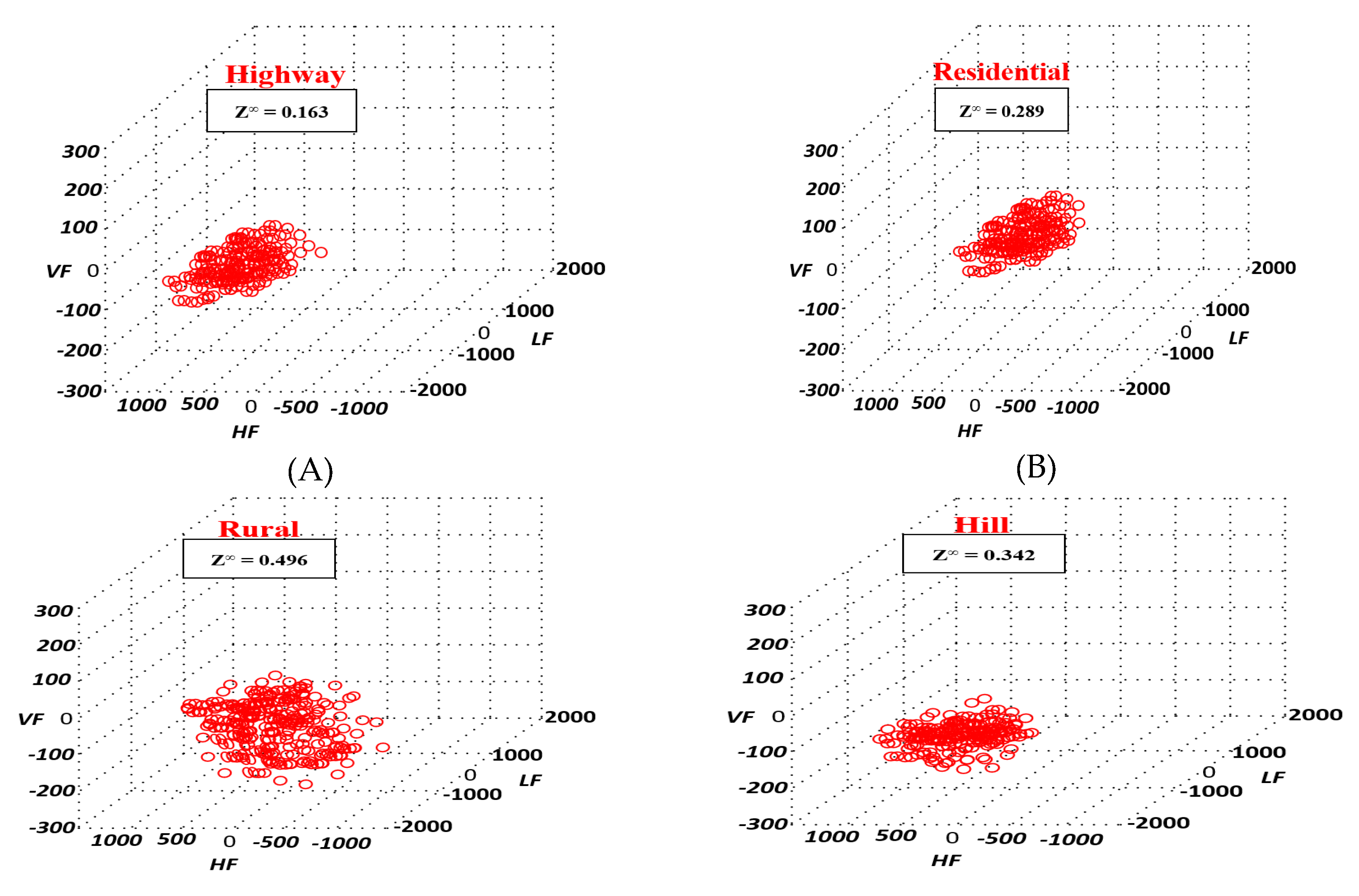
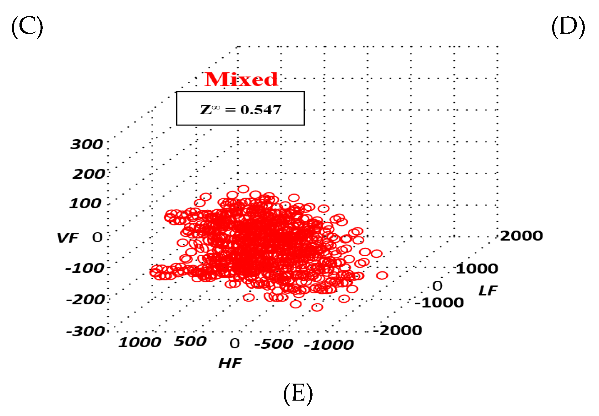
Upon doing the study using MATLAB®, the I-kaz Coefficient, denoted as Z
∞, was acquired for each route. The results were afterward shown in
Figure 17. According to the data shown in
Figure 17, it can be seen that the damage-surface road has the largest Z
∞ value, measuring 0.547 for the mixed road. This is followed by the rural road, which has a Z
∞ value of 0.496. Conversely, the highway displays the lowest Z
∞ value, amounting to 0.163. Furthermore, it is evident from the I-kaz display that the scattering space of the frequency distribution increases proportionally as the value of Z
∞ becomes larger. This implies that when the frequency of the fatigue signal increases, the value of Z
∞ also increases. This is the primary cause of the most significant dispersion of damage on the road surface. To conduct a comparison analysis, it is evident from the presented data in
Table 6 that larger values of Z
∞ correspond to higher levels of fatigue damage.
Table 7 presents the kurtosis and standard deviation values for highway, residential, rural, hill, and mixed roads. The statistical data were produced via the use of the Glyphworks program [
56]. According to the data presented in
Table 7, the kurtosis value for mixed roads was found to be greater than the kurtosis value for damaged roads. This phenomenon may be attributed to the observations made in
Figure 17, where it is evident that the rural and mixed road exhibited a higher degree of spikiness or transience compared to the damaged road, although having a smaller strain amplitude. This phenomenon may be attributed to the fact that kurtosis exhibits a high degree of sensitivity towards the presence of extreme values in the dataset. The fatigue damage of the coil spring was calculated using the GlyphWorks® program, while the analysis to derive the I-kaz coefficient and three-dimensional graphical representations of the collected fatigue signal from the road test was conducted using MATLAB® software as shown in
Figure 17.
Table 8 shows the comparison of fatigue damage cycles between this research and the literature where power spectra density (PSD) cycle counter, like Lalanne (LL), Dirlik (Di), and narrow band (NB) approaches are used,, additionally the table highlight the contribution, importance and the accuracy of the method used in this research.
7. Conclusions
This work presents a novel Digital Twin Model (DTM) that is both cost-effective and uncomplicated, designed specifically for Live Condition Monitoring (LCM) and Predictive Maintenance (PM). The suggested model is evaluated using a real-life case study. This study examined three distinct approaches used in fatigue analysis, including computational, experimental, and digital methodologies. The use of digital techniques in fatigue analysis is being employed for the first time. The used methodology yielded improved precision and allowed a comprehensive examination of the whole mechanical dynamics of the suspension system in real-time. This work presents an advancement in the dimensional modelling of the DT, reducing the number of dimensions from five to three. The purpose of this improvement is to provide a current and comprehensive assessment of the suspension system's state. The creation of the DTM involves three distinct aspects: Physical, Digital, and Connection. Despite its incorporation of these dimensions, the DTM remains very accurate and efficient. This study demonstrates a significant improvement in the predefined average load of simulation and experimental results, with an increase of 35.7%. Additionally, the average lifecycles of the system exhibited notable enhancements, surpassing the simulated and experimental results by 12 and 9 times, respectively. Furthermore, the implementation of the wired DTM showed a notable improvement in the average lifecycles of the system, with a 19.7% increase compared to the outcomes seen with the wireless DTM.
Future studies should focus on improving the techniques of data collection to meet the requirements of the DT model. As it is, the present data collection methods are inadequate. Therefore, it is necessary to revamp the conventional data collection approaches. The ultimate phase of the DT model involves the automated derivation and implementation of the conditions and interfaces pertaining to the physical entities, making them accessible for a diverse array of applications.
Author Contributions
The main author of this research paper is Dr Mohamed Ammar who did the study from inception to completion. Additionally, has played a significant role in conceiving and designing the research, collecting and analysing data, interpreting results, and writing and revising the manuscript. Specifically, has: Collaboratively formulated the research objectives and hypotheses, made the data collection, either through experiments, surveys, or data acquisition, conducted statistical analyses, and interpreted the findings jointly. All authors have read and agreed to the published version of the manuscript.
Funding Statement
The authors did not receive funding for this research study.
Acknowledgments
The authors would like to thank the Society of Automotive Engineers (SAE), for making the data available on their website.
Conflict of Interest
The authors declare that they have no conflicts of interest to report regarding the present study.
Availability of Data and Materials
The data and materials supporting the findings of this study are available at
https://www.sae.org/. We are committed to promoting transparency and facilitating further scientific inquiry, and we will make every effort to provide the necessary information and resources to interested parties in a timely manner.
References
- Ammar. M., Mousavi. A., Al-Raweshidy. H. (2023). Merging Artificial Intelligence with Digital Twins for Fault Prediction and Classification Using Suspension’s Primary Springs. International Journal of Advances in Electronics and Computer Science, 12, (10), 2394–2835.
- Boschert. S., Rosen. R. (2016). Digital twin-the simulation aspect. Mechatronic Futures: Challenges and Solutions for Mechatronic Systems and Their Designers, 2016, 59–74. [CrossRef]
- Hochhalter. JD., Leser. WP., Newman. JA., Glaessgen. EH., Cornell. SR., et al. (2014). Coupling Damage-Sensing Particles to the Digitial Twin Concept. NASA Technical Reports Server, 320, (4), 10.
- Růžička. M., Doubrava. K. (2005). Loading regimes and designing helical coiled springs for safe fatigue life. Research in Agricultural Engineering, 51, (2), 50–55. [CrossRef]
- Ammar. M., Mousavi. A., Al-Raweshidy. H. (2023). Digital Twins for Real-Time Condition Monitoring and Predictive Lifecycles of Primary Springs Used in Suspension Systems. International Journal of Mechanical and Production Engineering, 8, (11), 2321–2071.
- Ding. X., Selig. JM. (2004). On the compliance of coiled springs. International Journal of Mechanical Sciences, 46, (5), 703–727. [CrossRef]
- Jeong. K., Choi. S. (2019). Model-based Sensor Fault Diagnosis of Vehicle Suspensions with a Support Vector Machine. International Journal of Automotive Technology, 20, (5), 961–970. [CrossRef]
- Bartolozzi. R., Frendo. F. (2011). Stiffness and strength aspects in the design of automotive coil springs for McPherson front suspensions. Proceedings of the Institution of Mechanical Engineers, Part D: Journal of Automobile Engineering, 225, (10), 1377–1391. [CrossRef]
- Hu. H., Luo. H., Deng. X. (2021). Health Monitoring of Automotive Suspensions: A LSTM Network Approach. Shock and Vibration, 28, (9), 320–360. [CrossRef]
- Del Llano-Vizcaya. L., Rubio-González. C., Mesmacque. G., Cervantes-Hernández. T. (2006). Multiaxial fatigue and failure analysis of helical compression springs. Engineering Failure Analysis, 13, (8), 1303–1313. [CrossRef]
- Giovani. M., De Bortoli. D., Bosco. R., Puff. R. (2010). Fatigue Analysis of Helical Suspension Springs for Reciprocating Compressors. International Compressor Engineering Conference at Purdue, 4, (7), 111–130.
- Swanson. L. (2001). Linking maintenance strategies to performance. International Journal of Production Economics, 70, (3), 237–244. [CrossRef]
- Errandonea. I., Beltrán. S., Arrizabalaga. S. (2020). Digital Twin for maintenance: A literature review. Computers in Industry, 123, (6), 103316. [CrossRef]
- Peng. F., Ouyang. Y. (2012). Track maintenance production team scheduling in railroad networks. Transportation Research Part B: Methodological, 46, (10), 1474–1488. [CrossRef]
- Rahul Burgul. S., Kulkarni. AP. (2015). Fatigue Analysis for Helical Compression Spring for Determining Design Alternatives for Enhanced Life and Performance. International Journal For Technological Research In Engineering (IJTRE), 2, (7), 1070–1078.
- Tian. Z., Wong. L., Safaei. N. (2010). A neural network approach for remaining useful life prediction utilizing both failure and suspension histories. Mechanical Systems and Signal Processing, 24, (5), 1542–1555. [CrossRef]
- Animah. I., Shafiee. M. (2018). Condition assessment, remaining useful life prediction and life extension decision making for offshore oil and gas assets. Journal of Loss Prevention in the Process Industries, 53, (3), 17–28. [CrossRef]
- Wang. H., Peng. M jun., Miao. Z., Liu. Y kuo., Ayodeji. A., et al. (2021). Remaining useful life prediction techniques for electric valves based on convolution auto encoder and long short term memory. ISA Transactions, 108, (11), 333–342. [CrossRef]
- Wang. W., He. Q., Cui. Y., Li. Z. (2018). Joint Prediction of Remaining Useful Life and Failure Type of Train Wheelsets: Multitask Learning Approach. Journal of Transportation Engineering, Part A: Systems, 144, (6), 04018016. [CrossRef]
- Aye. SA., Heyns. PS. (2017). An integrated Gaussian process regression for prediction of remaining useful life of slow speed bearings based on acoustic emission. Mechanical Systems and Signal Processing, 84, (5), 485–498. [CrossRef]
- Tilahun. S., Velmurugan. P., Senthil Kumaran. S. (2020). Some Study onFatigue Life of Open Coil Suspension Spring. Journal of Critical Reviews, 7, (13), 139–143. [CrossRef]
- Tao. F., Cheng. J., Qi. Q., Zhang. M., Zhang. H., et al. (2018). Digital twin-driven product design, manufacturing and service with big data. International Journal of Advanced Manufacturing Technology, 94, (12), 3563–3576. [CrossRef]
- Martinez-Velazquez. R., Gamez. R., Saddik. A El. (2019). Cardio Twin: A Digital Twin of the human heart running on the edge. Medical Measurements and Applications, MeMeA 2019 - Symposium Proceedings, 6, (2), 139–146. [CrossRef]
- Donoghue. I., Hannola. L., Papinniemi. J., Mikkola. A. (2018). The benefits and impact of digital twins in product development phase of PLM. IFIP Advances in Information and Communication Technology, 540, (6), 432–441. [CrossRef]
- Hribernik. KA., Rabe. L., Thoben. KD., Schumacher. J. (2006). The product avatar as a product-instance-centric information management concept. International Journal of Product Lifecycle Management, 1, (4), 367–379. [CrossRef]
- Corcelle. C., Främling. K., Rabe. L., Anke. J., Petrow. J. (2007). Assessment of item-specific information management approaches in the area of heavy load vehicles. 4th International Conference on Product Lifecycle Management. Assessing the Industrial Relevance, 8, (1), 773–782.
- Hribernik. K., Wuest. T., Thoben. KD. (2013). A product avatar for leisure boats owners: Concept, development and findings. IFIP Advances in Information and Communication Technology, 409, 560–569. [CrossRef]
- Psarommatis. F., May. G. (2023). A standardized approach for measuring the performance and flexibility of digital twins. International Journal of Production Research, 61, (20), 6923–6938. [CrossRef]
- Yan. K., Lim. H., Zheng. · Pai., Chen. C-H., Zheng. P. (2020). A state-of-the-art survey of Digital Twin: techniques, engineering product lifecycle management and business innovation perspectives. Journal of Intelligent Manufacturing, 31, (7), 1313–1337. [CrossRef]
- Ammar. M., Al-Raweshidy. H. (2023). Integration of Digital Twins and Artificial Intelligence for Classifying Cardiac Ischemia. Journal on Artificial Intelligence, 5, (7), 195–218. [CrossRef]
- Sullivan. G., Pugh. R., Melendez. AP., Hunt. WD. (2010). Operations & Maintenance Best Practices - A Guide to Achieving Operational Efficiency (Release 3). U.S. Department of Energy under Contract DE-AC05-76RL01830, 19639, (3), 122–135. [CrossRef]
- Ahmed. AK., Al-raweshidy. HS., Member. S., Kh Ahmed. A. (2022). Performance Evaluation of Serial and Parallel Concatenated Channel Coding Scheme With Non-Orthogonal Multiple Access for 6G Networks. IEEE Access, 10, (4), 39681–39690. [CrossRef]
- Kh Ahmed. A., Al-Raweshidy. HS. (2023). Deep Learning Polar Convolutional Parallel Concatenated (DL-PCPC) Channel Decoding for 6G Communications. International Conference on Computer, Information and Telecommunication Systems (CITS), IEEE, 01–05. [CrossRef]
- Ramya. D., Bhargavi. B. (2018). Finite Element Analysis of Locomotive Primary Suspension by Using Composite Materials. Journal of Engineering Research and Application Www.Ijera.Com, 8, (9), 28–34. [CrossRef]
- Kamal. M., Rahman. MM. (2014). Finite element-based fatigue behaviour of springs in automobile suspension. International Journal of Automotive and Mechanical Engineering (IJAME), 10, (6), 1910–1919. [CrossRef]
- Safavi. S., Safavi. MA., Hamid. H., Fallah. S. (2021). Multi-Sensor Fault Detection, Identification, Isolation and Health Forecasting for Autonomous Vehicles. Sensors 2021, Vol. 21, Page 2547, 21, (7), 2547. [CrossRef]
- Akiniwa. Y., Stanzl-Tschegg. S., Mayer. H., Wakita. M., Tanaka. K. (2008). Fatigue strength of spring steel under axial and torsional loading in the very high cycle regime. International Journal of Fatigue, 30, (12), 2057–2063. [CrossRef]
- Zaccone. MA. (2001). Failure analysis of helical suspension springs under compressor start/stop conditions. Journal of Failure Analysis and Prevention, 1, (3), 51–62. [CrossRef]
- Pastorcic. D., Vukelic. G., Bozic. Z. (2019). Coil spring failure and fatigue analysis. Engineering Failure Analysis, 99, (4), 310–318. [CrossRef]
- Das. SK., Mukhopadhyay. NK., Kumar. BR., Bhattacharya. DK. (2007). Failure analysis of a passenger car coil spring. Engineering Failure Analysis, 14, (1), 158–163. [CrossRef]
- del Llano-Vizcaya. L., Rubio-González. C., Mesmacque. G., Cervantes-Hernández. T. (2006). Multiaxial fatigue and failure analysis of helical compression springs. Engineering Failure Analysis, 13, (8), 1303–1313. [CrossRef]
- Bartolozzi. R., Frendo. F. (2011). Stiffness and strength aspects in the design of automotive coil springs for McPherson front suspensions: A case study. Proceedings of the Institution of Mechanical Engineers, Part D: Journal of Automobile Engineering, 225, (10), 1377–1391. [CrossRef]
- Chin. CH., Abdullah. S., Singh. SSK., Ariffin. AK., Schramm. D. (2023). On the need to evaluate the probabilistic of fatigue life assessment of random strain loading considering load sequence effects. Engineering Failure Analysis, 145, (12), 107013. [CrossRef]
- Shah. QZ. (2023). study only focuses on the validation of the simulated strain signals through fatigue tests. Journal of Failure Analysis and Prevention, 11, (4), 324–344. [CrossRef]
- Kong. YS., Abdullah. S., Schramm. D., Omar. MZ., Haris. SM. (2019). Development of multiple linear regression-based models for fatigue life evaluation of automotive coil springs. Mechanical Systems and Signal Processing, 118, (9), 675–695. [CrossRef]
- Yang. T., Xue. S., Zheng. L., Liu. L., Liu. X. (2021). Fatigue Failure Analysis of Spring Coupling Diaphragm in Wind Power Generator. Journal of Failure Analysis and Prevention, 21, (6), 2143–2149. [CrossRef]
- Manouchehrynia. R., Abdullah. S., Singh. SSK. (2022). Fatigue-based reliability in assessing the failure of an automobile coil spring under random vibration loadings. Engineering Failure Analysis, 131, (6), 1350–6307. [CrossRef]
- Česnik. M., Slavić. J., Boltežar. M. (2012). Uninterrupted and accelerated vibrational fatigue testing with simultaneous monitoring of the natural frequency and damping. Journal of Sound and Vibration, 331, (24), 5370–5382. [CrossRef]
- Carpinteri. A., Spagnoli. A., Vantadori. S. (2003). A multiaxial fatigue criterion for random loading. Fatigue and Fracture of Engineering Materials and Structures, 26, (6), 515–522. [CrossRef]
- Del Llano-Vizcaya. L., Rubio-González. C., Mesmacque. G., Cervantes-Hernández. T. (2006). Multiaxial fatigue and failure analysis of helical compression springs. Engineering Failure Analysis, 13, (8), 1303–1313. [CrossRef]
- Kong. YS., Abdullah. S., Schramm. D., Omar. MZ., Haris. SM. (2018). Vibration fatigue analysis of carbon steel coil spring under various road excitations. Metals, 8, (8), 2322–2332. [CrossRef]
- Wang. CH., Brown. MW. (1996). Life Prediction Techniques for Variable Amplitude Multiaxial Fatigue—Part 1: Theories. Journal of Engineering Materials and Technology, 118, (3), 367–370. [CrossRef]
- Marsh. G., Wignall. C., Thies. PR., Barltrop. N., Incecik. A., et al. (2016). Review and application of Rainflow residue processing techniques for accurate fatigue damage estimation. International Journal of Fatigue, 82, (2), 757–765. [CrossRef]
- Amarnath. M., Lee. S-K. (2015). Assessment of surface contact fatigue failure in a spur geared system based on the tribological and vibration parameter analysis. Measurement, 76, (7), 32–44. [CrossRef]
- Chen. X. (2014). Analysis of crosswind fatigue of wind-excited structures with nonlinear aerodynamic damping. Engineering Structure, 74, (9), 145–156. [CrossRef]
- Tao. JX., Smith. S., Duff. A. (2009). The effect of overloading sequences on landing gear fatigue damage. International Journal of Fatigue, 31, (3), 1837–1847. [CrossRef]
- Chin. CH., Abdullah. S., Singh. SSK., Ariffin. AK., Schramm. D. (2020). Durability assessment of suspension coil spring considering the multifractality of road excitations. Measurement, 10, (12), 0263–2241. [CrossRef]
- Putra. T., Machmud. M. (2020). Predicting the fatigue life of an automotive coil spring considering road surface roughness. Engineering Failure Analysis, 116, (11), 1350–6307. [CrossRef]
- Manouchehrynia. R., Abdullah. S., Singh. S., Singh. K. (2019). metals Fatigue Reliability Assessment of an Automobile Coil Spring under Random Strain Loads Using Probabilistic Technique. Metals, 8, (7), 296. [CrossRef]
Figure 1.
Comparison of maintenance strategies with cost and frequency of maintenance.
Figure 1.
Comparison of maintenance strategies with cost and frequency of maintenance.
Figure 2.
Shows the spring fatigue testing machine for the experiment setup; (a) Helical spring with axial load. (b) free body diagram.
Figure 2.
Shows the spring fatigue testing machine for the experiment setup; (a) Helical spring with axial load. (b) free body diagram.
Figure 4.
Shows the fixed lower-end and the upper-end of the coil spring where the force is applied.
Figure 4.
Shows the fixed lower-end and the upper-end of the coil spring where the force is applied.
Figure 5.
Shows the final meshing modelling of the spring.
Figure 5.
Shows the final meshing modelling of the spring.
Figure 6.
Shows the flow process to create an actual and complete Digital Twin Model.
Figure 6.
Shows the flow process to create an actual and complete Digital Twin Model.
Figure 7.
Shows the process flow of the proposed Digital Twin Modelling concept.
Figure 7.
Shows the process flow of the proposed Digital Twin Modelling concept.
Figure 8.
Shows the channel setup on the IoT (Thingspeak) platform with a maximum of 8 fields (sensor) integration.
Figure 8.
Shows the channel setup on the IoT (Thingspeak) platform with a maximum of 8 fields (sensor) integration.
Figure 9.
shows the road profiles were categorised according to the prevailing road conditions.
Figure 9.
shows the road profiles were categorised according to the prevailing road conditions.
Figure 10.
Shows the spring constant variation with respect to the number of load cycles.
Figure 10.
Shows the spring constant variation with respect to the number of load cycles.
Figure 11.
Shows the fatigue curves of the springs under variable stress amplitude load.
Figure 11.
Shows the fatigue curves of the springs under variable stress amplitude load.
Figure 12.
Shows the absolute maximum principal stress distribution and fatigue life and damage plot for the triangular wave at 4 Hz.
Figure 12.
Shows the absolute maximum principal stress distribution and fatigue life and damage plot for the triangular wave at 4 Hz.
Figure 13.
Shows the Fatigue Life Distribution of 4.24*10^6 using Morrow’s model.
Figure 13.
Shows the Fatigue Life Distribution of 4.24*10^6 using Morrow’s model.
Figure 14.
Shows the Fatigue Life Distribution of 5*10^5 SWT’s model.
Figure 14.
Shows the Fatigue Life Distribution of 5*10^5 SWT’s model.
Figure 15.
Shows the measured acceleration-time history using different road conditions (a)highway, (b) residential, and (c) rural.
Figure 15.
Shows the measured acceleration-time history using different road conditions (a)highway, (b) residential, and (c) rural.
Figure 16.
Shows the measured strain-time history using different road conditions ((a)highway, (b) residential, and (c) rural.).
Figure 16.
Shows the measured strain-time history using different road conditions ((a)highway, (b) residential, and (c) rural.).
Figure 17.
Shows the I-kaz results and the I-kaz coefficients Z∞ for five road types.
Figure 17.
Shows the I-kaz results and the I-kaz coefficients Z∞ for five road types.
Table 1.
Shows the most recent failure analysis methods used in the literature and their limitations for coiled springs used in suspension systems.
Table 1.
Shows the most recent failure analysis methods used in the literature and their limitations for coiled springs used in suspension systems.
| Ref |
Method |
Limitations |
[43]
2023 |
Effective-Strain damage (ESD) model and Probabilistic approach for reliability evaluation |
ESD model estimated lower fatigue life than conventional models and the coil springs had lower fatigue reliability with load sequence |
[44]
2023 |
Development of a finite element model to justify and validate the outcomes of the study |
The study is limited to the analysis of extension springs and does not cover other types of mechanical springs. Does not explore the effects of environmental factors, such as temperature or humidity, on the failure of extension springs. The study is based on a case study analysis and may not capture the full range of failure mechanisms and scenarios that can occur in industrial applications. Does not address the impact of external factors, such as vibrations or shocks, on the failure of extension springs |
[45]
2022 |
Acoustic method fault detection system and Batch sampling method for quality check (QC) inspections |
The authors were unable to replicate the line density and noise peak observed in the reference experiment in their simulation. The complexity of the structure makes fault detection difficult and the Batch sampling method is not effective for detecting faults |
| [39] |
Multiple linear regression (MLR) and Strain-life models |
The evaluation of the proposed model is limited to comparing the predicted fatigue lives with measured strain fatigue life models, without considering other factors such as stress fatigue life approaches or real-world validation. |
| [46] |
Visual observations, optical and scanning electron microscopy
and hardness test |
Lacks detailed information on the specific conditions and factors that contributed to the fatigue failure of the valve springs. And lack of investigation into the root causes of the failure, such as the operating conditions, material properties, and design considerations |
| [47] |
FE Method for stress concentration factor evaluation |
Does not consider specific factors that caused the unexpected early fatigue failure of the component. Lacks information on the specific design modifications made to address the fatigue failure and meet the customer requirements. The analysis is based on simplified simulations and may not fully capture the complex behaviour of the component under actual operating conditions. |
| [48] |
Chemical composition analysis and mechanical property analysis |
Focuses primarily on the surface initiation of fatigue cracks and does not provide a comprehensive understanding of the underlying mechanisms and factors that led to the failure. Lacks information on the specific material properties and manufacturing processes of the spring diaphragm, which could have contributed to its susceptibility to fatigue failure. |
| [49] |
Microstructural analysis and fractography by SEM and Inclusion rating by optical microscopy |
The acquisition of a strain signal in traditional methods is constrained due to errors, time-consuming processes, and high costs. proposes a new method for generating strain signals based on computer simulation, but it does not address the challenges of acquiring strain signals in real-world scenarios |
Table 2.
Shows the Geometric And mechanical properties of the spring’s wire.
Table 2.
Shows the Geometric And mechanical properties of the spring’s wire.
| Properties |
Values |
| Density kg mm^-3 |
7.85e-006 |
| Young’s Modulus (E) MPa |
2.e+005 |
| Poisson’s Ratio |
0.3 |
| Bulk Modulus MPa |
1.6667e+005 |
| Shear Modulus MPa |
76923 |
| Tensile Yield Strength () MPa |
2270 |
| Tensile Ultimate Strength () MPa |
2950 |
| Fracture Strain () |
4.08% |
| Fracture Stress () |
2483 |
| Strain Hardening Component (n) |
0.0418 |
| Strength Coefficient MPa |
2916 |
| Strength Exponent |
-0.106 |
| Ductility Coefficient |
0.213 |
| Ductility Exponent |
-0.47 |
| Cyclic Strength Coefficient (K) MPa |
3322 |
| Cyclic Strain Hardening Exponent (n) |
0.088 |
| Cyclic Yield Strength () MPa |
1922 |
| Fatigue Strength Coefficient () MPa |
4108 |
| Fatigue Strength Exponent (b) |
-0.109 |
| Fatigue Ductility Coefficient () |
1.13 |
| Fatigue Ductility Exponent (c) |
-0.954 |
| Wire Diameter/mm |
11.5 |
| Mean Diameter of the spring/ mm |
110 |
| Coil’s Free Length/mm |
400 |
| Number of coils |
8 |
| Coil’s Pitch/mm |
43.00 |
| Wire diameter/mm |
11.5 |
| Mean diameter of the spring/ mm |
110 |
Table 3.
Shows the Hardware Components.
Table 3.
Shows the Hardware Components.
| *Dell Laptop |
*Peugeot 3008 car |
*Microcontroller: ATMEGA 2560 |
| *Load sensor |
*2mm strain gauges |
*Electric resistor using the Wheatstone bridge |
| *SoMat eDAQ |
*2mm electric wires |
*Voltage reader: HX711 amplifier for small voltage |
| *Wi-Fi module: DOIT ESP32 DEVKIT V1to transfer data to the server (ThingSpeak) |
Table 4.
Shows the load, deformation, and lifecycles resulting from the experimental method.
Table 4.
Shows the load, deformation, and lifecycles resulting from the experimental method.
| EXPERIMENTAL RESULTS |
|---|
| Load (KN) |
0.66 (Resembles Highway AVG) |
0.8 (Resembles Residential AVG) |
0.98 (Resembles Rural AVG) |
| Deformation(mm) |
36 |
43 |
49 |
| Stress (Mpa) |
155.7 |
168 |
214.3 |
| Lifecycles |
5.4*10^7 |
9.1*10^6 |
4.6*10^6 |
| AVG-load (KN) |
0.8 |
| AVG-lifecycles |
8.9*10^6 |
Table 5.
Shows load, deformation, and lifecycles resulting from the computational method.
Table 5.
Shows load, deformation, and lifecycles resulting from the computational method.
| COMPUTATIONAL |
|---|
| Characteristics |
Absolute |
CM |
Morrow |
SWT |
| Load (KN) |
0.66 |
0.74 |
0.8 |
0.98 |
| Deformation(mm) |
46.9 |
49.63 |
57 |
70.2 |
| Stress (Mpa) |
220 |
374 |
243.7 |
320 |
| Lifecycles |
4.24*10^6 |
3.33*10^6 |
5*10^5 |
2*10^5 |
| AVG-load (KN) |
0.8 |
| AVG-lifecycles |
6.6 *10^6 |
Table 6.
Shows the fatigue damage for each road based on CM, Morrow, SWT, and I-kaz.
Table 6.
Shows the fatigue damage for each road based on CM, Morrow, SWT, and I-kaz.
| Road Type |
Fatigue Damage |
| CM |
Morrow |
SWT |
I-Kaz |
| Highway (70 m/h) |
0.0059 |
0.0063 |
0.004 |
0.163 |
| Residential (30 m/h) |
0.006 |
0.0083 |
0.006 |
0.289 |
| Rural (25 m/h) |
0.285 |
0.465 |
0.316 |
0.946 |
| Hill (50 m/h) |
0.693 |
0.069 |
0.471 |
0.342 |
| Mixed (5 -70 m/h) |
0.932 |
0.570 |
0.864 |
0.547 |
Table 7.
Shows the statistical parameters obtained from acceleration and strain time history.
Table 7.
Shows the statistical parameters obtained from acceleration and strain time history.
| Parameters |
Highway |
Residential |
Rural |
Hill |
Mixed |
| Statistical Parameters from Acceleration-Time History for Different Road Profiles |
| Mean (m/s^2) |
0.006 |
0.005 |
0.044 |
0.082 |
0.142 |
| RMS (m/s^2) |
0.866 |
0.584 |
0.448 |
0.332 |
0.122 |
| Kurtosis (m/s^2) |
3.232 |
4.842 |
4.462 |
3.432 |
5.231 |
| Standard Deviation |
60.462 |
82.446 |
94.222 |
89.653 |
99.623 |
| Crest Factor |
05.45 |
08.22 |
11.84 |
07.37 |
84.32 |
| Statistical Parameters from Strain-Time History for Different Road Profiles |
| Mean (m/s^2) |
0.019 |
0.015 |
0.044 |
0.132 |
0.252 |
| RMS (m/s^2) |
210.95 |
509.26 |
748.91 |
310.23 |
832.58 |
| Kurtosis (m/s^2) |
3.316 |
4.332 |
5.732 |
3.946 |
5.642 |
| Standard Deviation |
48.645 |
63.247 |
71.723 |
61.278 |
82.662 |
| Crest Factor |
7.34 |
11.35 |
23.34 |
9.23 |
6.45 |
Table 8.
Shows a comparison of fatigue damage cycles between this research and the literature.
Table 8.
Shows a comparison of fatigue damage cycles between this research and the literature.
| Ref |
Method |
Fatigue Life Cycles |
| High |
Res |
Rur |
Hill |
Mix |
2023
[43] |
CM |
X |
X |
X |
X |
X |
| Mo |
109
|
105
|
105
|
106
|
X |
| SWT |
1010
|
105
|
105
|
106
|
X |
| I-kaz |
X |
X |
X |
X |
X |
2022
[47] |
LL |
9.8× 10⁶
|
1.51 × 10⁸
|
4.09 × 10⁶
|
X |
X |
| Di |
2.6× 10⁸
|
1.51 × 10⁸
|
6.02 × 10⁶
|
X |
X |
| NB |
1.4× 10⁶
|
1.32 × 10⁶
|
1.00 × 10⁶
|
X |
X |
2020
[57] |
CM |
8.073 |
5.600 |
4.835 |
X |
6.732 |
| Mo |
8.393 |
5.728 |
4.684 |
X |
6.536 |
| SWT |
8.839 |
5.808 |
4.608 |
X |
6.434 |
2020 [58]
|
CM |
X |
X |
X |
X |
X |
| Mo |
X |
X |
X |
X |
X |
| SWT |
X |
X |
X |
X |
X |
2019 [59]
|
CM |
3 × 10⁵
|
2 × 10⁵
|
2 × 10⁵
|
X |
X |
| Mo |
2 × 10⁵
|
7 × 10⁴
|
3 × 10⁴
|
X |
X |
| SWT |
1 × 10⁵
|
3 × 10⁴
|
2 × 10⁴
|
X |
X |
| I-Kaz |
X |
X |
X |
X |
X |
2018 [51]
|
LL |
2.7× 10¹⁷
|
2.2× 10¹¹
|
1.8× 10⁷
|
X |
X |
| Di |
5.2× 10¹⁷
|
6.5× 10¹¹
|
4.4× 10⁷
|
X |
X |
| NB |
7.1× 10¹⁶
|
2.2× 10¹¹
|
5.6× 10⁶
|
X |
X |
| I-kaz |
X |
X |
X |
X |
X |
| This Research |
CM |
5.9×10⁻³
|
6×10⁻³
|
28.5×10⁻²
|
69.3×10⁻²
|
93×10−2
|
| Mo |
6.3×10⁻³
|
8.3×10⁻³
|
46.5×10⁻²
|
6.9×10⁻²
|
57×10−2
|
| SWT |
4×10⁻³
|
6×10⁻³
|
31.6×10⁻²
|
47.1×10⁻²
|
86×10−2
|
| I-Kaz |
0.16 |
0.29 |
0.95 |
0.34 |
0.547 |
|
Disclaimer/Publisher’s Note: The statements, opinions and data contained in all publications are solely those of the individual author(s) and contributor(s) and not of MDPI and/or the editor(s). MDPI and/or the editor(s) disclaim responsibility for any injury to people or property resulting from any ideas, methods, instructions or products referred to in the content. |
© 2024 by the authors. Licensee MDPI, Basel, Switzerland. This article is an open access article distributed under the terms and conditions of the Creative Commons Attribution (CC BY) license (http://creativecommons.org/licenses/by/4.0/).
