Preprint
Article

Estimating Monetary Demand Using a Flexible Model of Almost Ideal Demand System(AIDS)

Altmetrics

Downloads

119

Views

43

Comments

0

This version is not peer-reviewed

Submitted:

20 June 2024

Posted:

24 June 2024

You are already at the latest version

Alerts
Abstract
Money demand is the amount of real money balance with people and they can decide at any time what part of their assets to keep in cash. In this study, money was assumed to be a durable good that leads to the flow of some kind of service. Therefore, money became a function of utility. Using AIDS elasticity demand function, income, price and cross elasticities were evaluated. The statistics of this study are related to the years 2003-2022. The results showed that, based on the assumption of three goods, the demand includes bills and negotiable instruments, demand deposits, and time deposits. Based on the limitation of symmetry, collectability and homogeneity, the tensions can be calculated. The results showed that the price elasticity of demand for banknotes and muskox with term deposits is not significant. On the other hand, the cross tension between sight deposits and term deposits is negative and significant.
Keywords: 
Subject: Business, Economics and Management  -   Economics

1. Introduction

Money in macroeconomics is often defined positively by its functions in society because it analyzes the behavior of economic groups and their reactions to changes in economic variables. From this point of view, the nature of money is not important, but its function in society is. Investigating the money demand function from the perspective of macroeconomic analysis and economic policy-making is of great importance (Azizi et al, 2011). A correct and accurate understanding of this function, which includes all the fundamental and influential variables, provides the necessary ground for the successful application of economic policies (Falahati et al, 2019). In other words, the demand for money means that people tend to keep what part of their assets at any given time is in the form of cash or money. The demand for money does not mean the flow of money and spending it on daily running expenses, but rather the demand for the balance of money at any time. In the process of reducing interest rates by monetary authorities, people tend to increase the demand for money, and in fact, sometimes reducing interest rates does not satisfy them because, in this case, the opportunity cost of holding money has decreased.Usually, at low interest rates, the incentive to hold money in cash increases and the tendency to buy securities increases, so there is an inverse relationship between the interest rate and the demand for money (the demand for the real balance of money), (Azizi and Torkamani, 2001). Additionally, you can also check when the rates are rising. Under these circumstances, the opportunity cost of holding money increases, and the desire to hold money in the form of cash decreases. Therefore, we say that the demand for money decreases when interest rates rise, and some people try to keep their bank savings deposits (Branson, 1994).
Studies in developed countries indicate that the demand for money is subject to a variety of interest rates in addition to income (Azizi and Yazdani, 2007). However, developing countries play a role in the demand for money due to the lack of proper financial markets, exchange rates, and inflation rates, along with real income.
In the last few decades, money was defined only as all monetary assets on which no interest was accrued. These financial assets included cash and bank deposits, but today's individual portfolios also include additional financial assets like term savings deposits, etc. that provide holders with varying rates of return. In our research, using the combination of the micro theory and the aggregation theory of Barnett (1977), we estimate the demand function of money in Iran, in which money is viewed as a durable commodity that has led to the acquisition of a flow of services (Dobnik, 2013).
As a result, money enters the utility function. We will be able to solve the issues associated with monetary aggregation by utilizing flexible functional forms and demand systems.
In this regard, we will use Diort's findings on the use of flexible forms (Azizi, 2015).
In an in-depth look at the selection of functional forms for estimating the systems of producer and consumer supply and demand functions, Diort tries to find functional forms that are compatible with the constraints of supply and demand functions (which imply economic theories) and, in addition, have sufficient flexibility that can be associated with the constraints of supply and demand functions. The choice of the functional form and the elasticities of supply and demand should not be arbitrarily restricted (Mane, 2012).
Finally, to provide a strategic model for the demand for money, it is necessary to recognize people's behavioral patterns and provide questions based on behavioral patterns to have the highest degree of effectiveness in decisions (Jabbari et al, 2024). In this study, we try to calculate income, insider, and crossover elasticities quarterly during the period from 2003 to 2023 and model people's behavior in the face of the current conditions. In the rest of the article, in the second part of the theoretical literature, the background of the research will be presented. In the third part, the methodology of the research will be discussed. The fourth part of the research includes the estimation of the model.

2. Theoretical Foundations and Litrature Review

2.1. Theoretical Foundations

Economic agents usually keep money for two purposes: to store value and to conduct transactions. Generally, economic instability affects the amount of money these brokers are willing to hold. For example, an increase in interest rate volatility and an increase in the risk of inflation make all nominal assets risky. This is because the value of these types of goods and services is less predictable. Thus, in an unstable inflationary environment, economic actors can convert their nominal assets, including money, into other assets such as gold (Atta Mensa, 2004).
The money demand function plays an important role in understanding the transmission of changes in the money supply and other variables, such as interest rates, to the economy (Azizi et al, 2024). Since the 1930s, economists have put forward theories in order to determine the factors that hold money.
Fischer(1911) and Pigo (1917) showed that there is a direct and proportional relationship between the amount of money and the level of price in the form of classical equilibrium. These two emphasize the role of money as a medium of exchange in transactions. In the theory of quantity of money, the demand for money is not precisely discussed, but it is the trading speed of the circulation of money that is emphasized (Zara-Nejad et al, 2006).
In the Fisher exchange relationship, the amount of money in circulation for a given period is related to the level of full employment and the exchange price of P t for a given period through the speed of the trading circulation of V t . Fisher assumes that in the short term, the speed of money circulation is constant and that the amount of money is determined independently of the trading volume. On the other hand, in the framework of equilibrium based on classical full employment, it is assumed that there is a constant rate between the level of transactions and production: Therefore,we have:
M t   .   V t = P t   . Y t  
In the Cambridge approach, Marshall(1923) stated that the level of holding money is related to the number of transactions. When people's wealth increases, they hold more financial assets, one of which is money (Kuan et al, 2012).
M t = K . P . Y
In this regard, k represents the tendency of people to keep a portion of their income in the form of money, which is the opposite of the speed at which money circulates, except that here it refers to the speed at which people convert their money into commodities (Bedrom, 1999).
Keynes argues that people hold money because of three motives: transactional, precautionary, and speculative. Following Fisher and Cambridge economists, Keynes (1936) argues that the transactional demand for money is a constant function of income. On the other hand, in addition to holding money for their current transactions, people also hold some money in order to meet their needs and expected payments in the future. which is known as precautionary motivation (Khalili Iraqi, 2005).
The difference between Keynes's view of money and other views on the speculative demand for money is that it shows the relationship between the demand for money and the interest rate. He states that people hold a combination of money and bonds that have yields. In such a way that the expectation of an increase in the interest rate in the future will increase the speculative demand for money, and conversely, the liquidity preference function of Keynes is:
M P = F   y , r
In this function, the real demand for money is a function of income and interest rate
Baumol (1952) and Tobin (1956) sought to introduce a theory in which money is essentially an entity that is held for a transactional purpose. Although financial assets other than money have a higher return than money, the transaction cost of converting financial assets into money when needed justifies holding money.
The household asset portfolio consists of two asset groups: assets that have returns and generate income, and money that covers the gap between payments and receipts. Transaction costs are incurred when non-monetary assets are sold to finance the transaction. In this case, holding more money minimizes the transaction cost and, on the other hand, causes a loss of interest income. The optimal point, which can yield the minimum trading cost and the maximum interest for individuals, is determined based on the following relationship (Fallahi, 2005):
M d s p = a . y 2 r
M d s p ،a، y، and r represent optimal demand for money, transaction costs, real income, and interest rates, respectively (Dehmardeh et al, 2009).
Friedman(1956) believes that people keep money in order to buy the services and goods they need. He states that because money is a durable commodity with invisible services, it enters into the functions of desirability and production. On the other hand, money is compared to other assets such as bonds, stocks, and durable goods. In such a way that if the amount of money held increases, the ultimate desirability of monetary services decreases. In summary, Friedman emphasizes two points: first, he does not consider the expected rate of return of money to be fixed, and assuming that the demand for money also depends on the motivation to hold other assets, he states that the demand for money does not show sensitivity to changes in the interest rate. So if the interest rate increases, because the expected rate of return of money held in the form of bank deposits will also increase, it will not have much effect on reducing the incentive to hold money. Therefore, changes in interest rates do not have a significant effect on the demand for money, and it is only the permanent income of individuals that affects their demand for money (Farzin et al, 2012).
M P = ( y p )
Secondly, Friedman, unlike Keynes, believes that the demand for money function is stable, which means that the amount of money demanded can be predicted by the demand for money function, and on the other hand, the speed of money circulation is completely predictable due to the insensitivity of the demand for money to the interest rate (Khalili et al, 2013).
Nowadays, the demand for money is studied over both short- and long-term periods. Obviously, an increase in the amount of money demand in the long run can only occur as a result of an increase in the amount of production in a country. Therefore, if the amount of domestic production increases in society and there is a demand for the purchase of these products, then the central bank will face an increase in the demand for money and will issue money, which will result in price stabilization and economic growth.
Otherwise, and with the continuation of the issuance of money regardless of the country's production trend, it will have no effects other than inflationary pressure. However, in long-term studies of money demand, the increase in the amount of domestic production, which is sometimes interpreted as economic dynamism, is measured using the index of industrial production, or GDP (Snowden, 2010).

2.2. Litrature Review

In this section, the empirical studies conducted in the field of estimating the money demand function and the factors affecting it over different time periods have been examined.
Kuan Payne and Jones(2012) investigated the stability of the short-run money demand function in the United States for the period 1959–1981. The results of the fitted regression equation for the period could not confirm the test of the transfer hypothesis in the money demand function in the United States in 1971, and the results indicated the stability of the money demand function for the period under consideration.
Prakash et al.(2012) investigated the money demand function based on the Naranslog function model in Malawi and its policy strategies. For this purpose, it was tried to estimate the money demand function for the period 1985–2010 using annual data and econometric methods. During the period under study, several structural failures occurred in the economy of this country. It showed the existence of a long-run relationship between real money balances, prices, income, the exchange rate, Treasury bonds, and financial innovations. However, all variables have a significant impact on the demand for money in the short and long run. Therefore, policy-making should be done in order to increase financial innovation, improve economic activities, and achieve higher returns.
Lee and Chang(2012), investigated the money demand function in China based on an explanatory model with bounded distributional lags. For this purpose, they used the data between 1976 and 2006 and the mentioned model. Their results showed that there is a long-run relationship between the limited definition of money, real income, and the nominal interest rate. It was equal to 0.915 and -0.0002 for the Chinese economy, respectively.
Prakash and Manoj, (2012) investigated whether there is a stable, long-term relationship between money demand in India. For this purpose, they used the Georg-Hansen model for the period 1953–2008. The results of the co-combination test showed that there is a long-run relationship between money demand, real GDP, and the nominal interest rate, despite the structural failure in 1965. The results also showed a downward movement of the demand function by 0.33% in 1965.
Kumar et al. (2010) investigated the level of stability of money demand in Nigeria during the period 1960-2008 using error correction models and stability test of the money demand function of this country. The results of their research showed that the demand for money is efficiently stable, so the policymakers of this country can use the money supply as a policy tool.
Bafandeh Imandoost and Ghasemi (2011) investigated the factors affecting Iran's money demand under uncertain conditions for the period between 1975 and 2006. In this paper, they used the Bayesian model averaging method to consider the uncertainty assumption of the model due to its appropriate features. Gross Domestic Product (GDP), Price Index of Goods and Services, Official Exchange Rate, Budget Deficit to GDP, Dependent Variable with Interruption, and Price Index of Goods and Services with Interruption.
Dehmardeh and Izadi (2009) investigated the money demand function in Iran. The purpose of this study was to estimate the money demand function in Iran for the period 1971–2008 using the ARDL method and to investigate the relationships between independent and dependent variables. The results showed that there is a long-run equilibrium relationship between the variables in this estimate. The coefficient of the GDP variable indicates a positive and significant effect of this variable on the money demand function. On the other hand, the relationship between free market exchange rate variables and inflation on the money demand function was negative and indicated an inverse and significant effect between these variables and the dependent variable.
Khalili et al, (2013) studied the demand for money in Iran using error correction and collage models during the years 1971–2011. Based on the estimated relationship and the income elasticity coefficient of the demand for money with a 1% increase in GDP, the demand for cash balance increases by 1.82%. The estimated coefficient for the exchange rate (-0.34) indicates the substitution of domestic and foreign currencies. The long-term interest rate coefficient is significant and indicates the negative interest elasticity of money demand in Iran. Also, the results of the stability test showed that the demand for money during this period is stable.

3. Methodology

3.1. Almost Ideal Demand System (AIDS)

The Almost Ideal demand system (AIDS) was first introduced by Dayton and Müllbor in 1980. In this demand system, a specific set of preferences called pig log[1] are used. Piglog preferences are extracted from the following expense function:
L n   C u , p = 1 u l n a   p + u   l n b p
where u is the desirability and p is the price vector. In this function, a and b are positive linear homogeneous functions of the price vector, and the desirability of u is between zero (minimum livelihood) and 1 (maximum happiness). Thus, the functions a(p) and b(p) are the necessary expenditures to achieve the minimum livelihood and maximum happiness, respectivel. In order for the above expenditure function to ultimately be a flexible form of function, it must have sufficient parameters to have its derivatives at any desired point. For this purpose, specific functional forms are considered, as follows (Al-Emran et al, 2010):
ln a   ( p ) = a 0 + k = 1 n ln p k + 1 2 k = 1 n j = 1 n β k j * ln p k ln p j  
ln b   p = ln a   ( p ) + β 0 k = 1 n p k β k  
Now, by substituting the relations 7 and 8 in relation (6), the flexible expenditure function is given as follows (Azizi, 2015):
ln c   u   ,   p = a 0 + k = 1 n ln p k + 1 2 k = 1 n j = 1 n β k j * ln p k ln p j + u β 0 k = 1 n p k β k
Now, in order for the expenditure function in terms of prices to be linearly homogeneous, it must be c   u   ,   p
The following constraints should be applied to the equation:
i = 1 n a i = 0
j = 1 n β k j * = k = 1 n β k j * = j = 1 n β j = 0  
It can be easily shown that the relationship (9) is flexible due to having sufficient parameters, and since desirability is a rank quantity, it can always be normalized so that we have at a given point:
2   L n c ( u , p ) u 2 = 0
In fact, the relationships (7) and (8) have been chosen in such a way that they can create a flexible form that leads to a system of demand functions with arbitrary properties, which we will refer to below. The demand function is derived from the derivative of the expenditure function relative to prices (Azizi, 2010):
c ( u , p ) p i = x i  
By multiplying the two sides by the expression p i c ( u   ,   p ) We will get the phrase s j :
c ( u , p ) p i . p i c ( u , p ) = l n c u , p l n p i
where s i is the share of the commodity i in the budget. Thus, by deriving the function (9) with respect to the logarithm of each of the prices, the share of each commodity in the budget is obtained as a function of price and utility:
s i = ln c ( u   ,   p ) l n p i = a 0 + j = 1 n β i k * ln p k + β 1   u β 0 k = 1 n p k β k
  β 1 k = 1 2 ( β i k * + β k i * )
For consumers who are at a point of self-optimization, the total expenditure (income) y is equal to c (u, p). By inverting this function, the indirect utility function u will be obtained in terms of p and y. So if we solve relation (4) in terms of u and substitute the result in relation (14), The budget share will be obtained as a function of p and y, which is the same system of AIDS demand functions in the form of budget share equations:
s i = a i + k = 1 n β i k * ln p k + b i   l n y ln P
where lnP is the Tratslog price index and is defined as follows:
l n P = a 0 + k = 1 n a K ln p k + 1 2 k = 1 n j = 1 n β k j * ln p k ln p j  
Note: In some cases, the Stone Gray index is used to calculate P, which is calculated as follows:
ln p = i = 1 n s i ln p i    
In equation (16), is the budget share of the i commodity, y is the income, is the price of the k commodity, and (a,b,β) are the parameters of the demand system that are estimated, and the symmetry constraints are as follows:
β i j = β j i for   all   I , j
and homogeneity constraints as:
j i n β i j = o   for   all   I
are applied in estimation.
Assuming j = 1 and there are n goods, the share equations in the AIDS model will have n 2 + 3 n 2 / 2   free parameters.
As long as the relative prices p k and real expenses do not change, the budget shares will also remain the same, and the forecast is started using this model based on this assumption. β i k shows the effect of changes in relative prices on the budget share. The effect of real expenditure changes on the budget share of commodity i is shown by coefficient b i ; this coefficient will be positive for luxury goods and negative for essential goods.

4. Discussion

In estimating the country's money demand function system using the AIDS and Leontief models, we consider the three monetary components used in this section as follows: using the demand values of each of the components and the cost of using each of them, we estimate the demand function of approximately what we will pay.
  • Banknotes and cash registers
  • Visual deposits
  • Term deposits
The data and information used in this study were extracted from the balance sheet of the Central Bank (2003–2022) and economic indicators (2003–2022). The variables are: banknotes and coins, visual deposits, term deposits, implied price index, and active population. The data are collected quarterly, and the period under study is from 2003 to 2022, with a total of 44 for each variable (World Bank, 2023). We will observe. Since in this study we need a sample to analyze the results more accurately, to calculate the per capita value of each component of money, we divided its values by the active population, and on the other hand, in order to achieve real prices and de-inflation, we divided the nominal price (cost of use) of each component in different seasons by the consumer price index (CPI) published by the Central Bank.

4.1. Model Estimation

4.1.1. Model Estimation Using AIDS Model

In this section, we will rewrite the AIDS model and the constraints mentioned in the previous section for the three-commodity mode that is considered in this article. The limitations of symmetry, aggregation, and homogeneity in the three-commodity state are:
β i j = β j i
1 + 2 + 3 = 1
β 1 j + β 2 j + β 3 j = 1
β i 1 + β i 2 + β i 3 = 1
b 1 + b 2 + b 3 = 1  
According to equation number (16), the number of eight parameters ( α 0 , α 1 , α 2 , b 1 , b 2 , β 11 , β 12 , β 22 ) should be estimated.
Based on the estimation of the above parameters, the other parameters of the model are estimated using the constraint set as follows:
β 13 = β 11 β 12
β 23 = β 12 β 12
β 33 = β 11 + 2 β 12 + β 22
α 3 = 1 α 1 α 2
b 3 = b 1 b 2
According to what was stated in the previous section and using the constraints of the relationship (21) in the case of three goods, it is enough to estimate only two equations. For this purpose, we consider the equations for the share of the components as follows:
s 1 = a 1 + β 11 ln p 1 + β 12 ln p 2 β 11 + β 12 l n p 3 + b 1 l n y l n p  
s 2 = a 2 + β 12 ln p 1 + β 22 ln p 2 β 12 + β 22 l n p 3 + b 2 l n y l n p  
The Translog price index in the three-commodity mode will be as follows:
Preprints 109946 i005
In the next step, the share equations are estimated using the seemingly unrelated regression method using Eviews software.

4.1.2. Results of Reliability Tests

Therefore, in order to prevent the occurrence of the phenomenon of false regression during the estimation of the model, it is necessary to first examine and test the stationarity of the variables, as stated in the chapter on the research method. Special tests of this type of data can be used to investigate the reliability of the variables in the panel data. Here are two tests, Lin & Levine (LL) and M. Sons & Shin (IPS), which are more commonly used to investigate the reliability of variables in combined data, The tests were determined by Eviuse 6 software and by significance based on Prob at the level of 5%. Since the H 0 hypothesis of the test indicates the existence of a unit root for each variable, if the calculated P-value is less than 5%, the hypothesis of the existence of a unit root for that variable is rejected. The results of the variable durability test are shown in Table 1.
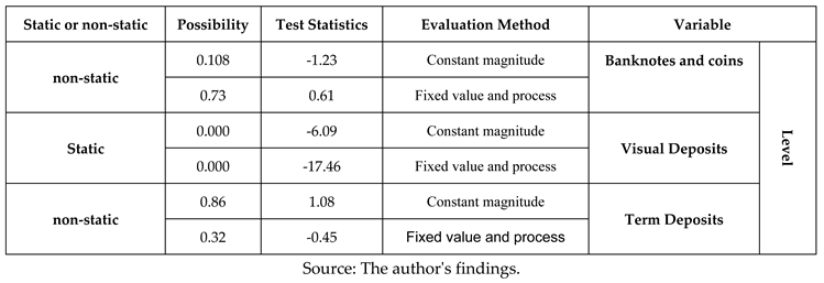
Based on the results of Table 1 and the Lin, Levine, and Chow tests, all variables are at the static level. To ensure the results obtained by the LL test, the results of the static test of the variables by the methods of Im, Son, and Shin are also presented in Table 2.
According to the results of Table 2, the two variables of banknotes and coins and term deposits are non-static, but the variable of visual deposits is at a static level. However, based on the EM test, the sons and shein of banknotes, coins, and term deposits are static with a one-time differential, as follows:
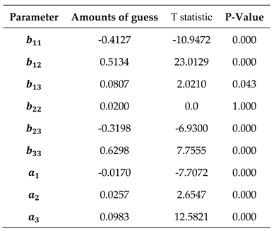
Here are the results of the estimate. The results are shown in Table 4, along with the t-statistic and P-value.
As can be seen, the AIDS model provides a good fit between the three portfolios of monetary assets under study, so that except for one parameter, the rest of the parameters are significant. This model was used as the basis for elasticity analysis.

5. Results

Money in macroeconomics is often defined positively by its functions in society because it analyzes the behavior of economic groups and their reactions to changes in economic variables. In this study, we try to calculate income, insider, and crossover elasticities quarterly during the period from 2003 to 2023 and model people's behavior in the face of the current conditions. In the rest of the article, in the second part of the theoretical literature, the background of the research will be presented. In the third part, the methodology of the research will be discussed. The fourth part of the research includes the estimation of the model. The data and information used in this study were extracted from the balance sheet of the Central Bank (2003–2022) and economic indicators (2003–2022). The variables are: banknotes and coins, visual deposits, term deposits, implied price index, and active population. Money demand is the amount of real money balance with people and they can decide at any time what part of their assets to keep in cash. In this study, money was assumed to be a durable good that leads to the flow of some kind of service. Therefore, money became a function of utility. Using AIDS elasticity demand function, income, price and cross elasticities were evaluated. The statistics of this study are related to the years 2003-2022. The results showed that, based on the assumption of three goods, the demand includes bills and negotiable instruments, demand deposits, and time deposits. Based on the limitation of symmetry, collectability and homogeneity, the tensions can be calculated. The results showed that the price elasticity of demand for banknotes and muskox with term deposits is not significant. On the other hand, the cross tension between sight deposits and term deposits is negative and significant.

References

  1. Al-Imran, R.; Nasrollah, F.; Al-Imran, S.A. Investigating the Effect of the Economic Stability Index on Money Demand in Iran. J. Appl. Econ. 2010, 1, 71–98. [Google Scholar]
  2. Atta-Mensah, J. The Demand for Money in a Stochastic Environment. Bank of Canada Working Paper No. 2004.7. 2004. [CrossRef]
  3. Azizi, J. , Esmaeilpoor, F. and Taleghani, M. (2010). Effect of the Quality Costing System on Implementation and Execution of Optimum Total Quality Management. International journal of Business and Management (CANADA). Vol.5.No.8. [CrossRef]
  4. Azizi, J.; Aref Eshghi, T. The Role of Information and Communication Technology (ICT) in Iranian Olive Industrial Cluster. J. Agric. Sci. 2011, 3, 228–232. [Google Scholar] [CrossRef]
  5. Azizi, J. Evaluation of the Efficiency of the Agricultural Bank Branches by Using Data Envelopment Analysis and the Determination of a consolidated index: The Case Study MAZANDARAN Province. Iran. J. Agric. Econ. 2015, 9, 63–76. [Google Scholar]
  6. Azizi, J.; Torkamani, J. Estimation Of Demand Function For Different Types Of Meat In Iran: Application Of Cointegration. EQTESAD-E KESHAVARZI VA TOWSE'E https://www.sid.ir/en/Journal/ViewPaper.aspx?ID=22226. 2001, 9, 217–238. [Google Scholar]
  7. Azizi, J. , and Yazdani, S. (2007). Investigation stability income of export date of Iran.
  8. Azizi, J.; Vahabi Sorood, M.; Mohammadinejad, A. Influential Elements Influencing How Consumers Behave when Purchasing Organic Farm Products. Preprints 2024, 2024060611. [Google Scholar] [CrossRef]
  9. Bafandeh Imandoost, Sadegh, and Ghasemi, Hessameddin (2011), "Investigating the Factors Affecting Iran's Money Demand Using Bayesian Averaging Approach," Financial Monetary Economics, No. 1, pp. 37–57.
  10. Branson, William (1994). Macroeconomics (translated by Morteza Emadzadeh), Tehran, Islamic Azad University Scientific Publishing Center.
  11. Baumol, W.J. The transaction demand for cash: an inventory theoretic approach. Q. J. Econ. 1952, 545–556. [Google Scholar] [CrossRef]
  12. Dehmardeh, N.; Izadi, H.R. A Study of the Demand Function of Money in Iran. Q. J. Econ. Stud. 2009, 9, 153–169. [Google Scholar]
  13. Farzin-Vash, A.; Samadi Boroujeni, R. Measuring the Welfare Cost of Inflation in Iran. Eghtesadi J. 2012, 12, 7–18. [Google Scholar]
  14. Fallahi, M.A.; Neghdari, E. Investigating the Factors Affecting Money Demand in Iran's Economy with an Emphasis on Exchange Rate (Application of the ARDL Model). J. Knowl. Dev. 2005, 147–166. [Google Scholar]
  15. Falahati, S.; Azizi, J. Role of Rural Markets in Rural People’s Economic Prosperity in Guilan Province of Iran. Village Dev. 2019, 22, 125–139. [Google Scholar] [CrossRef]
  16. Fridman, M. The Demand for Money, Some Theoretical and Empirical Results. J. Political Econ. Univ. Chic. Press 1959, 67, 185–191. [Google Scholar] [CrossRef]
  17. Jabbari, Afsaneh and Azizi, Jafar, Analysis of the Demand for Dairy: The application of the NBR model (June 2, 2024). Available at SSRN: https://ssrn.com/abstract=4851510. [CrossRef]
  18. Keynes, J. M. (1936). The general theory of interest, employment, and money.
  19. Khalili Araghi, Mansour, Abbasnejad, Hossein, and Goudarzi Farahani, Yazdan (2013). "Estimating the Money Demand Function in Iran Using Error Correction and Correlation Models," Journal of Monetary and Financial Economics (formerly Knowledge and Development), New Period, Vol. 20, No. 5, pp. 1–26.
  20. Lin, K.-P.; Oh, J.S. Stability of the U.S. Short-Run Money Demand Function, 1959–81. J. Financ. 2012, 39, 1383–1396. [Google Scholar]
  21. Kumar, Saten, Webber, Don J., and Fargher, Scott (2010), “Money demand stability: A case study of Nigeria," MPRA Paper 26074, University Library of Munich, Germany, pp. 1–28.
  22. Lee, C.-C.; Chang, C.P. The Demand for Money in China: A Reassessment Using the Bounds Testing Approach. J. Econ. Forecast. 2102, 74–94. [Google Scholar]
  23. Lungu, M.; et al. Money demand function for Malawi: implications for monetary policy conduct. Banks Bank Syst. 2012, 7, 50–63. [Google Scholar]
  24. Marshall, A. (1923). Money, credit, and commerce.
  25. Pedroni, P. Critical values for cointegration tests in heterogeneous panels with multiple regressors. Oxf Bull Econ Stat 1999, 61, 653–670. [Google Scholar] [CrossRef]
  26. Singh, P.; Pandey, M.K. Is Long-Run Demand for Money Stable in India? An Application of the Gregory-Hansen Model," the IUP. J. Appl. Econ. 2012, 6, 59–69. [Google Scholar]
  27. Snowden, Brian (2004). A New Guide to Macroeconomics (Translated by Ali Souri, Mansour Khalili Iraqi), Brothers.
  28. Tobin, J. The interest-elasticity of transactions demands cash. Rev. Econ. Stat. 1956, 241–247. [Google Scholar] [CrossRef]
  29. World Bank (2023), “World Development Indicators 2023”. worldbank.org.
  30. Zara-Nejad, M.; Anvari, E. Estimation of the Hedonic Price Function of Housing in Ahvaz City Using Mixed Data Methods. Q. J. Econ. Res. 2006, 8, 138–168. [Google Scholar]
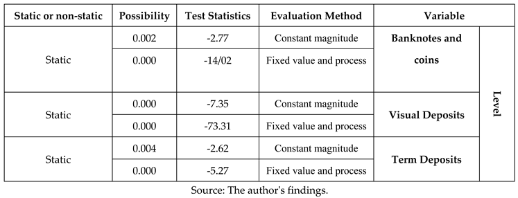
Table 1. Results of the Static Test of Variables by the Levin, Lin, and Chow Methods (Surface).
Preprints 109946 i001
Table 2. Results of the Static Test of Variables by I, Boys, and Shin Methods (Level).
Preprints 109946 i002
Table 3. Results of the Static Test of Variables by the I, Boys, and Shin Methods (First Difference).
Preprints 109946 i003
Table 4. Results of estimating the model parameters.
Preprints 109946 i004
Disclaimer/Publisher’s Note: The statements, opinions and data contained in all publications are solely those of the individual author(s) and contributor(s) and not of MDPI and/or the editor(s). MDPI and/or the editor(s) disclaim responsibility for any injury to people or property resulting from any ideas, methods, instructions or products referred to in the content.
Copyright: This open access article is published under a Creative Commons CC BY 4.0 license, which permit the free download, distribution, and reuse, provided that the author and preprint are cited in any reuse.
Prerpints.org logo

Preprints.org is a free preprint server supported by MDPI in Basel, Switzerland.

Subscribe

© 2024 MDPI (Basel, Switzerland) unless otherwise stated