1. Introduction
As one of the most popular fruits and vegetables, tomato is widely grown around the world [
1]. Greenhouse planting is regarded as the first choice by many tomato growers, and the greenhouse planting scale is expanding constantly [
2]. Compared with planting in the field, the growing season of tomatoes planted in the greenhouse can be extended to protect tomatoes from the influence of abiotic factors caused by weather changes and provide a safe and suitable growth environment for tomatoes [
3]. With the improvement in quality of life, the pursuit of tomato quality is more and more high, i.e., high degree of freshness, ruddy color of tomato rich in vitamins with higher nutritional value, which is beneficial to the physical and mental health of the human body and can also bring higher economic benefits [
4,
5]. Since the ripening process of tomatoes is divided into green ripening stage, white ripening stage, turning color stage, red ripening stage and complete ripening stage [
6], the color feature is a good indicator to identify the maturity of tomato [
7]. The tomatoes in green ripening stage are no longer bulked, and this is the earliest picking stage, which is suitable for long-distance transportation. Turning color stage and red ripening stage are suitable for short distance transportation and nearby supply, and complete ripening stage is only suitable for nearby supply. Abiotic stresses, such as temperature, have an important impact on plant growth and development [
8,
9]. Temperature is one of the important factors affecting the synthesis of lycopene, and the color of tomato is directly affected by the content of lycopene [
10].
Precise management of color and shape transformations during each stage of tomato growth can facilitate agricultural laborers in accurately harvesting tomatoes at various stages of development based on market freshness, transportation and storage conditions, thereby ensuring the nutritional quality of the produce [
11,
12]. Environmental factors such as temperature, light intensity, and soil temperature exert a significant impact on the phenotype of plants [
13]. By conducting phenotypic studies on tomato fruits, one can clearly display their external morphological characteristics and visualize their growth process to record environmental indicators that affect tomato growth. This enables researchers to study the growth cycle of tomatoes and determine optimal harvesting time. Therefore, it is highly valuable to integrate environmental factors in predicting the external phenotypic traits of tomatoes, specifically their color and shape based on historical periods. In this paper, the Internet of Things (IoT) technology is used to collect the color and shape of tomato fruit as real-time data to dynamically predict tomato growth trend.
Labor is liberated to some extent through the use of IoT technology in agricultural [
14], such as monitoring the growth and health status of plants [
9,
15]. Ting et al. proposed the photosynthesis prediction model on the basis of the SVM model for the entire growth stage of tomato, a wireless sensor network-based was used for the real-time monitoring of environmental factors [
16]. Harun et al. proposed using the IoT technology for remote monitoring to improve the growth of Brassica chinensis and increase yield [
17]. Liao et al. have developed a set of IoT based monitoring system for environmental factors in orchid greenhouse and monitored the growth of phalaenopsis orchids [
18]. Studies combining environmental factors with plant growth and development are conducive to the development of precision agriculture [
19], and related research has been carried out at home and abroad [
20,
21]. Jiang et al. proposed using LSTM for corn production prediction, using multiple neural networks (Recurrent Neural Networks) to a cycle model, namely to more than one month for training as input to predict the output of the next month [
22]. Kocian et al. proposed to use dynamic Bayesian networks to connect indicator parameters of crop development with environmental control parameters through hidden Markov states to predict crop growth. This method can only predict the dynamic changes of a single phenotype of plants, and the plant growth process cannot be visualized [
19].
The above research is mainly aimed to predict the change trend of a future time point, howerer, the growth and development of plants cannot be directly observed. Therefore, in this study the multi-input multi-output model is proposed, which uses multiple historical data to predict multiple tomato states in the future. Meanwhile, the intuitive two-dimensional image time series for prediction is used to visualize the growth process of tomato fruits. Two-dimensional image time series describes both time and space information, including not only the time information of the sequence before and after, but also the spatial information of the target on the image and the movement and change of the target. Compared with the current research using mask image prediction, the texture and color information of the image is more fully utilized [
23].
In this study, environment condition information is obtained through the use of sensors, tomato growth status is monitored in real time through a camera, and tomato images are collected. The model of tomato fruit color transformation is constructed and the historical data is used to predict the future growth of tomato. Starting with fruit color and shape those directly reflect tomato ripening, a fruit growth model driven by environmental data is established to study the time required for tomato to complete ripening stage from green ripening stage under different environment conditions. And then exploring methods to abbreviate the ripening cycle of tomatoes and establishing a suitable model for their growth. It provides data support for the establishment of tomato plant growth and development model in solar greenhouse.
2. Experimental Design and Data Construction
2.1. The Location of the Experiment
The experiment site is located in the tomato solar greenhouse (E117.166°, N36.174°) in the science and technology industrial Park of Shandong Agricultural University (Panhe Campus). The greenhouse is a new-type solar greenhouse with a length of 70 m from east to west, a span of 9.8 m from north to south, a depth of 0.5 m, a rear wall height of 3.8 m and a ridge height of 5 m. The wall is reinforced with brick and soil base cement. The transparent covering material is light transmittance strong drip-free polyethylene film, the covering quilt is made of waterproof rainproof silk outer cover and fiber cotton inner core. It is equipped with two air vents, the lower one is located 60 cm above the ground, and the upper one is located at the top of the greenhouse, with a width of 1.3 m.
2.2. Tomato Cultivation and Management
Spring tomato is used as the experiment content, and the experiment tomato variety is “Sheng Luo Lan 3689”, which has developed root system, strong plant, anti-virus, anti-dead tree, low temperature resistance and other characteristics, suitable for planting in northern regions. The plant has vigorous growth, rounded fruit type, high yield, many branches in the ear, strong fruit setting ability, large and uniform fruit, single fruit weight of 240-300 grams, high fruit hardness and suitable for transportation. Tomatoes are transplanted on February 24, 2021, with a plant spacing of 17.5 cm and a row spacing of 160 cm, and a density of about 2400 plants per 666.7 m
2. The plants are dried and pruned individually, and the seedlings are drawn on June 30, 2022. The growth cycle totaled 124 days, including 36 days for seedling stage, 19 days for flowering and fruit setting, and 69 days for fruit setting. The division of the growth cycle is shown in
Table 1.
During the period, tomato water fertilizer, spray and daily management shall be carried out according to the conventional management methods of the park, without special treatment. Since the tomato has unlimited growth, plants and fruits grow in parallel, and the competition for nutrition is very fierce, two leaves are left after five spikes to top, the water, fertilizer, spraying and daily management of tomato are carried out according to farmers’ planting experience. This paper mainly focuses on the study of tomato fruiting period, and its agricultural management is shown in
Table 2 and
Table 3.
2.3. Design of Data Acquisition System for IoT
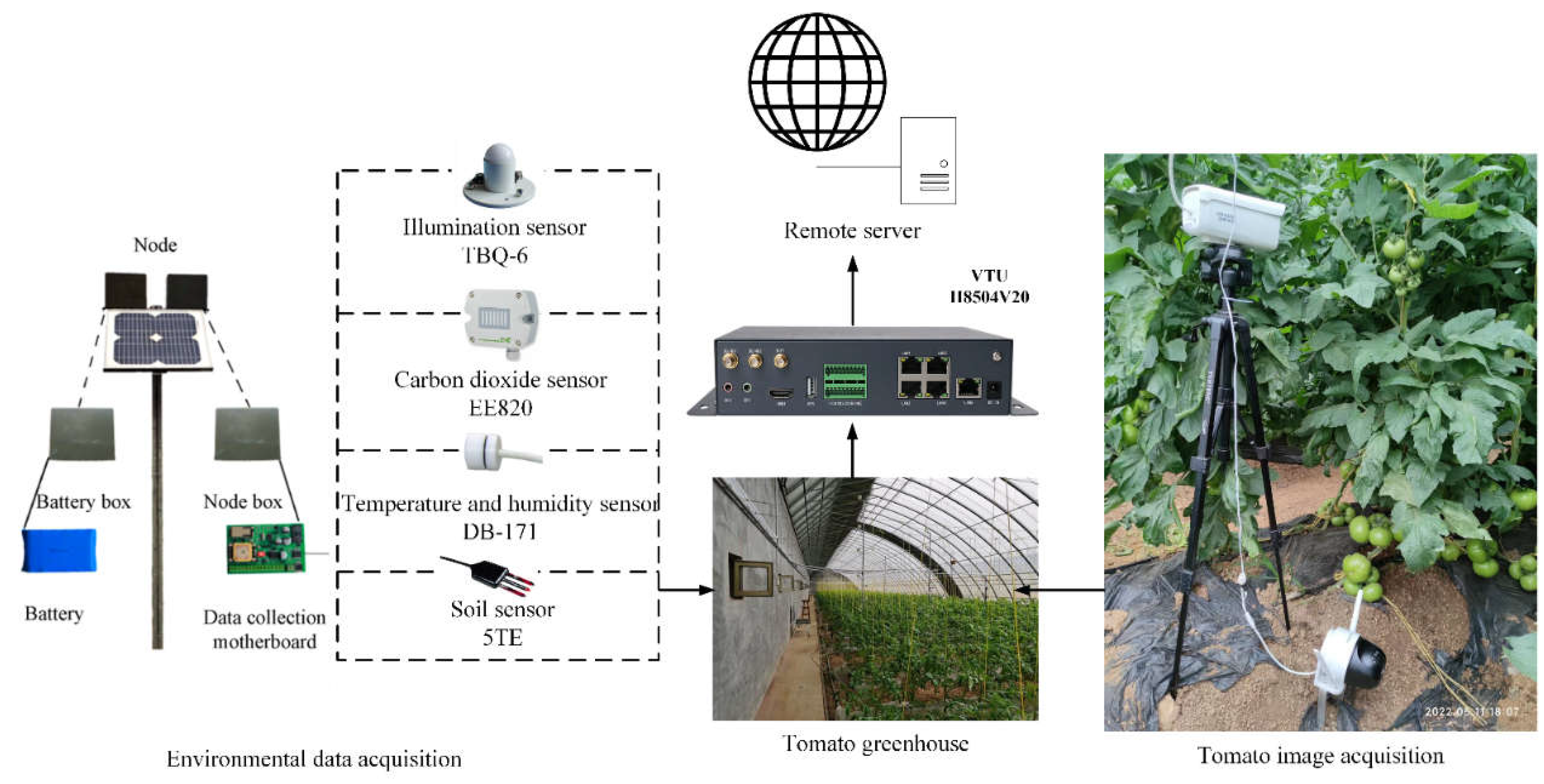
The IoT environment data acquisition system is mainly composed of CPU, perception module and transmission module. The core of coordinating the work of each module and ensuring the stable operation of the system is CPU, which can realize the functions of data storage, data analysis, and data interaction. The sensing module realizes accurate perception of air temperature, humidity and light intensity through external sensing equipment. The transmission module uploads the collected information to the server in real time through the IoT transmission device. Parameters of the IoT sensors are shown in
Table 4. 5G network Dahuale orange TS2F camera is selected for image data acquisition, with a resolution of 4 million HD, rotating with head, including levelness and verticality, supporting full-color night vision. Data acquisition system architecture is shown in
Figure 1.
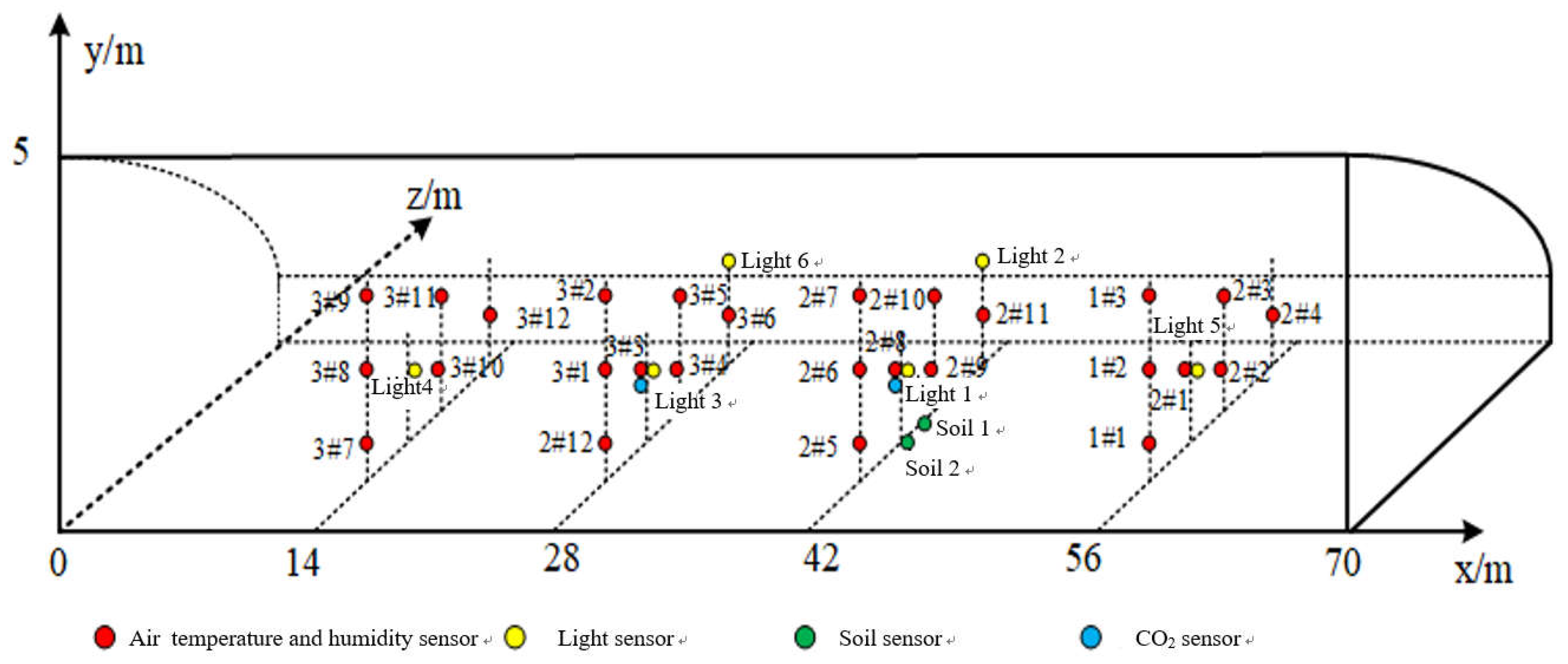
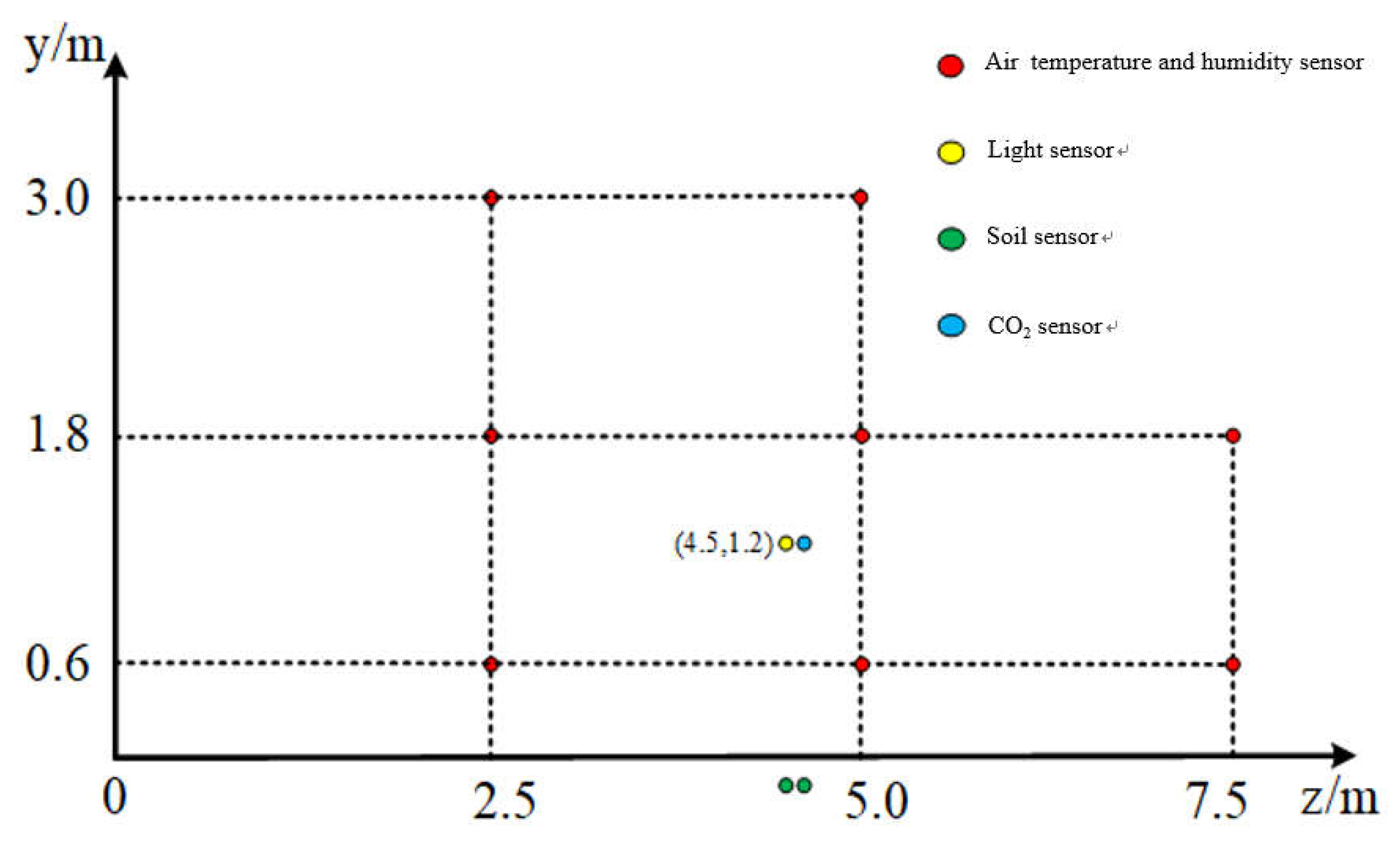
To reduce the measurement error of the sensors and ensure the effective monitoring of the greenhouse environment, multiple groups of sensors are uniformly distributed in the greenhouse. In the height direction, the sensors are arranged in the 0.6 m, 1.8 m and 3.0 m planes, respectively. In the north-south direction, the greenhouse is divided into four parts with 2.5 m as a unit, and sensors are arranged at 2.5 m, 5 m and 7.5 m respectively. In the east-west direction, the greenhouse is divided into five parts in units of 14 m, and sensors are placed at 14 m, 28 m, 42 m, and 56 m, respectively. The stereo diagram and side view of the sensor deployment point are shown in
Figure 2 and
Figure 3, respectively.
2.4. Tomato Image Preprocessing and Data Set Production
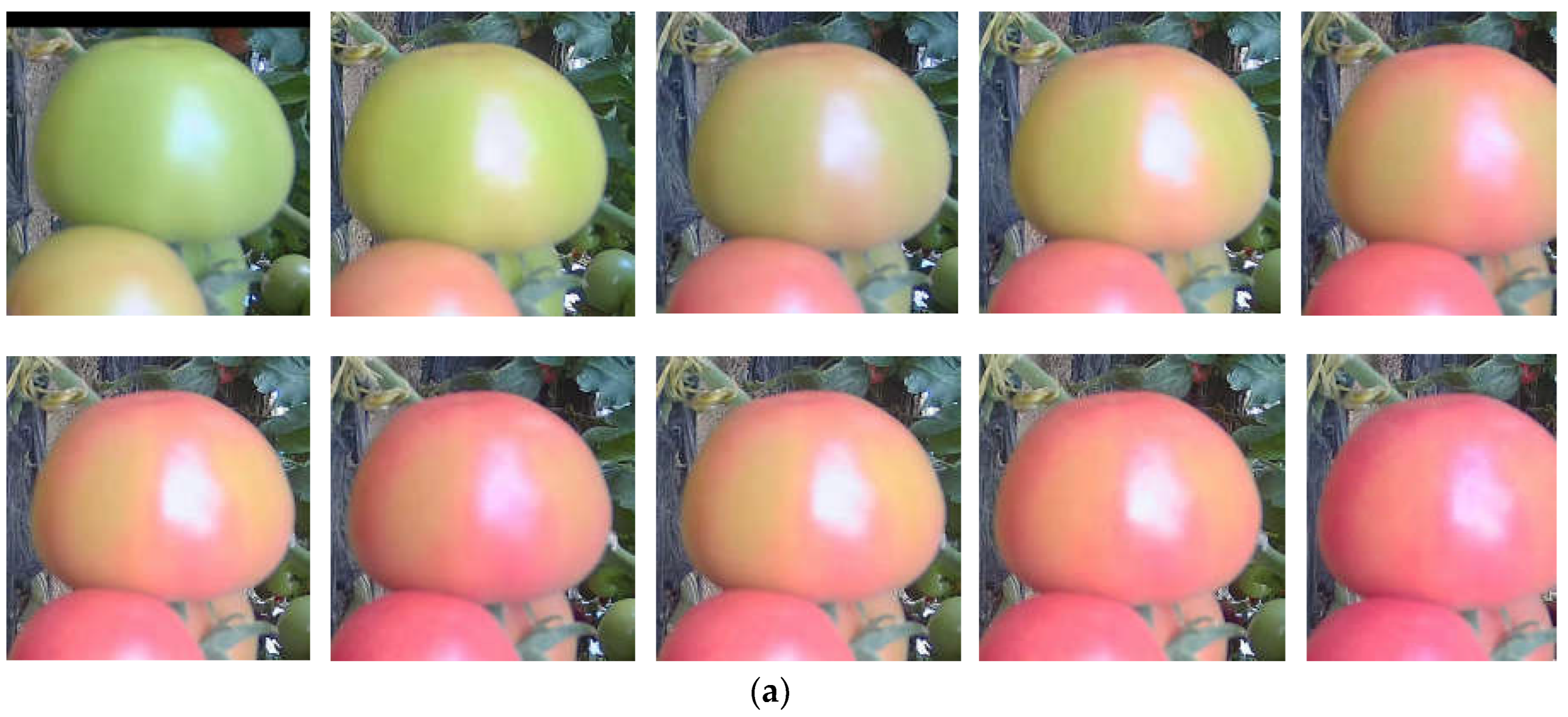
The image data was collected from green ripening stage to complete ripening stage. Real-time monitoring was conducted by Dahualle Orange TS2F camera equipment, and the collected image sequences were collected every 4 hours. A total of 49 image sequences were retained, and each sequence contained 10 image data. Adjust the tomato image size to 128 pixels×128 pixels. The .json files obtained by Labelme annotation were converted into mask .png files in batches to obtain the tomato mask images to reduce the interference of background noise. The tomato images before and after removing the background are shown in
Figure 4. To enhance the richness of the data, the original data are rotated and enhanced by 90°, 180° and 270°. The 1960 image data after data enlargement were numbered in chronological order, with numbers 1-5 as input sequences and numbers 6-10 as output sequences, among which 1600 were training data and 360 were validation data.
3. Spatial-Temporal Prediction Model
With the passage of time, tomato color will change dynamically in space dimension. Compared with traditional data, tomato color is dependent in time dimension and space dimension, so it is necessary to consider the influence of different positions in space. Therefore, tomato growth data set belongs to spatial-temporal series data [
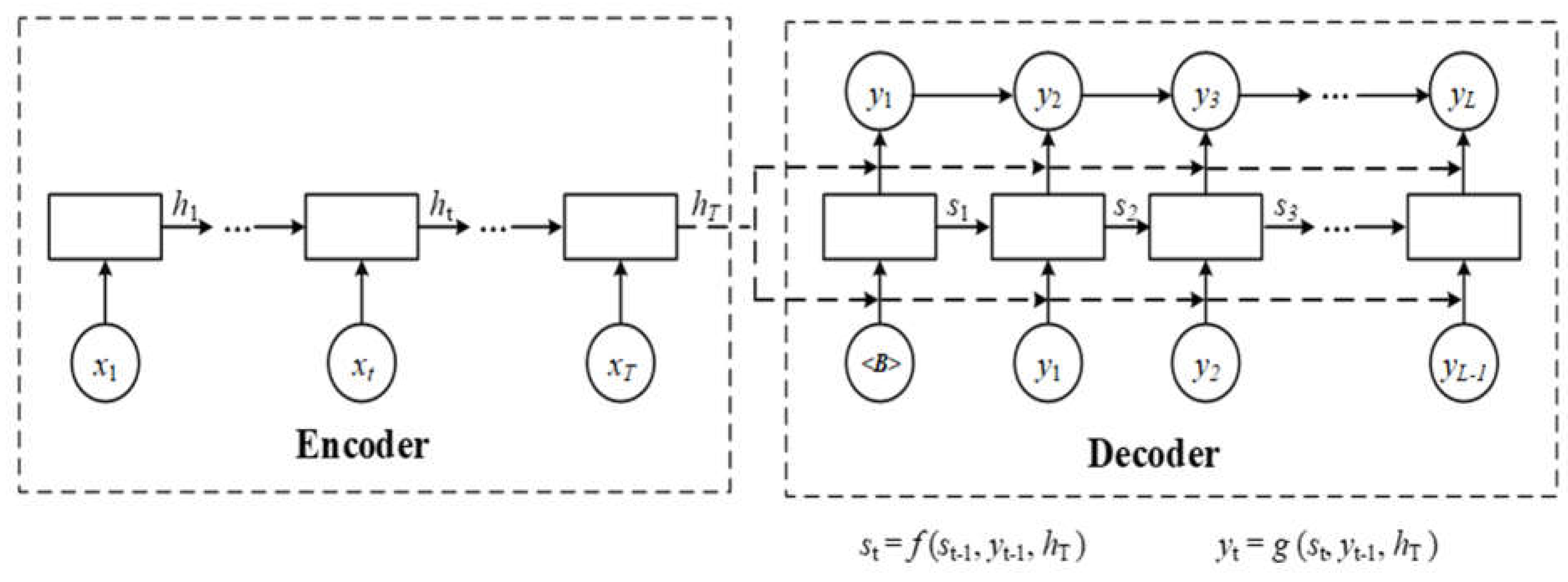
24]. To take into account both time and space dimensions, Zaremba et al. propose the RNN structure, which can deal with the problem of spatial-temporal series prediction. A schematic representation of a typical structure of an RNN encoder-decoder is shown in
Figure 5. However, RNN is prone to the problems of gradient disappearance and gradient explosion, so it only has short-term memory [
25]. The introduction of long short term memory network (LSTM) solves the problem of RNN, but the internal structure of LSTM is complex and the training efficiency is low. The emergence of gated recurrent unit network (GRU) solves the above problems. In this paper, the dependent variable is set as tomato color while the independent variable is air temperature. To fully utilize spatial-temporal information, historical data of tomatoes are analyzed to predict future growth states through multi-step spatial-temporal prediction. Additionally, a two-dimensional image representation of tomato growth data set is studied to reflect its growth state in an intuitive manner.
The image sequence at time t is defined as
, where
denote the width, height and channel of the image respectively. Historical
tomato images
are given to predict
future tomato images
, the prediction of tomato growth state is expressed by formula (1),
denotes the maximum likelihood function.
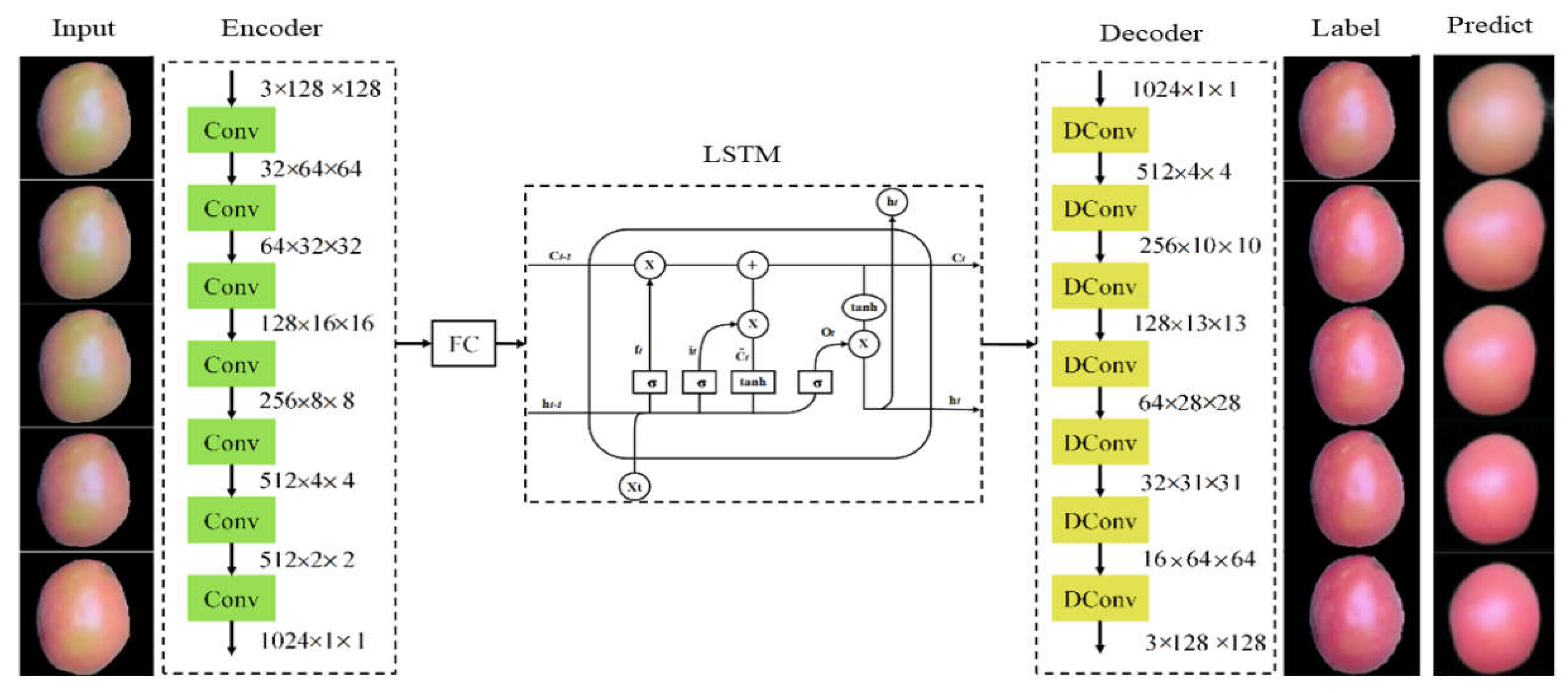
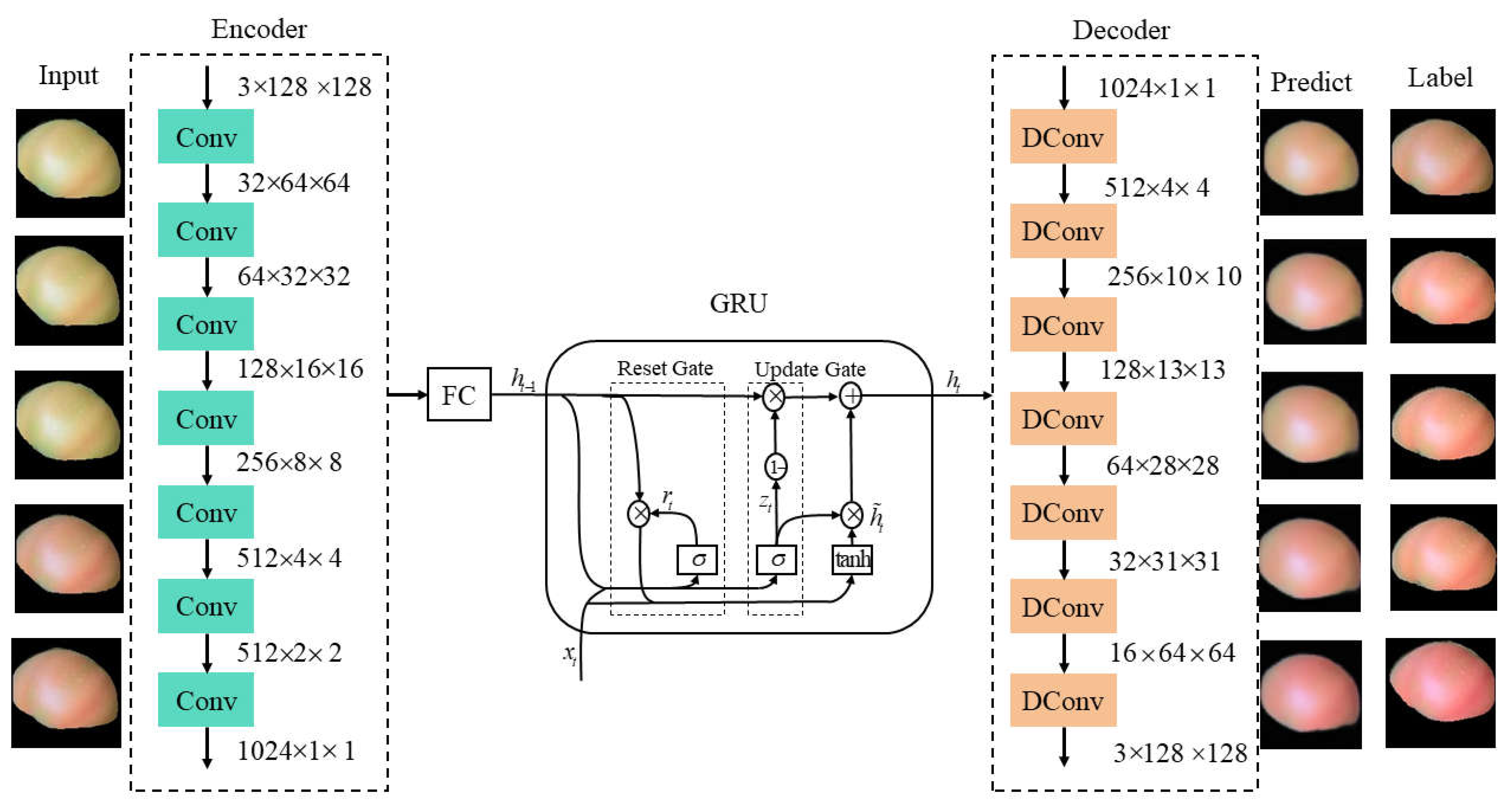
In this paper, LSTM and GRU composed of encoder-decoder are used to predict the growth of tomato. The encoder-decoder structure can encode the growth pattern of tomato and effectively simulate the tomato growth phenotype. The encoder structure is to convert the original input signal into intermediate representation, and the decoder structure is to convert the intermediate representation into the target output. Here, the encoder structure is composed of 7 convolutional layers, and the convolutional layer is used to process the input picture and convert the picture form into intermediate representation, i.e., the time and space features of the input data sequence are extracted, and the output is used as the input of the GRU layer. The GRU layer is used to remember the tomato state and establish time dependence. Deconvolution is used in the decoder structure to convert the intermediate representation into two-dimensional image form for output.
3.1. LSTM Networks
The activation function of LSTM network is the identity function with derivative of 1.0, and the problem of gradient disappearance and gradient explosion in the process of long sequence training of RNN can be solved [
26,
27]. LSTM resolves the problem of long-term dependence through gate units, which includes forgetting gate, input gate and output gate. Compared with traditional RNN network, LSTM also has a neural unit state used to store historical information. However, the internal structure of LSTM unit is complex, which requires a long time for training [
28].The structure of LSTM is shown in
Figure 6, and the work flow is described by formula (2)-(7).
denotes cell state at the current moment, represents cell state at the previous moment, denotes cell state update value, represents forgetting gate, is the input gate, is the output gate, is the sigmoid activation function, is the hyperbolic tangent activation function, represents bias entry, denotes input, denotes LSTM output of the current hidden layer, denotes output of the hidden layer before LSTM, represents weight matrix.
3.2. GRU Network
Due to the complex structure, many parameters, high time cost, waste of computing resources and other problems of LSTM network, this paper chooses GRU whose performance is equivalent to that of LSTM network. The structure is shown in
Figure 7. GRU is an improvement of LSTM [
29], which simplifies the internal structure of LSTM by simplifying the three gate structures of LSTM into two gate structures of reset gate and update gate. This operation reduces the parameters required for training, and determines the weight of historical data series through the control of the gate. The convergence speed of the model is fast, and the training time is shortened. Among them, the function of the update gate is to control the historical information transmitted from the previous point in time to the current point in time, and the reset gate determines the degree of historical information being forgotten [
29]. The calculation of the gated cycle unit network is shown in Formula (8)-(11):
denotes input, stands for reset gate, represents the update gate, represents the reset gate weight matrix, represents the update gate weight matrix, represents candidate hidden state weight matrix, represents hidden layer output, represents candidate hidden status.
4. Experimental Results and Analysis
4.1. Experimental Platform
The computer hardware configuration used in the experiment is as follows: The operating system is Windows 10, wherein the CPU is Intel(R) Core (TM) i5-8400 CPU @ 2.8GHz ~2.81GHz, NVIDIA GeForce RTX 3060 Ti, and the software framework is python 3.7.
4.2. Model Training
The L1 is used as the loss function, Adam is used as the optimizer, and the ReduceLROnPlateau learning rate is used as the attenuation strategy. The initial learning rate is set to 8, and the batch size is set to 8. To prevent overfitting, the dropout technology is introduced and the early stop strategy is used on the verification set. Different hidden layer number, hidden unit number and different RNN structures are selected to discuss the effect of the model on predicting the tomato growth. The RNN structures are LSTM and GRU, respectively, to select the optimal results.
4.3. Results and Analysis
Selection of structural similarity Structural Similarity Index Measure (SSIM) evaluation index to evaluate the proposed model for tomato, similarity between data forecast with the actual image SSIM is to better measure to predict tomato overall visual image quality. The closer the SSIM is to 1, the more similar the two images are in contrast, brightness and structure [
30].
Table 5 shows the indexes of the LSTM and GRU models of encoder and decoder structure. The SSIM value of the GRU model is 0.008 higher than that of the LSTM model of encoder-decoder structure. The size of the model is reduced by 30 MB, and the model is easier to train.
4.3.1. Influence of Different Network Structures on the Prediction Performance
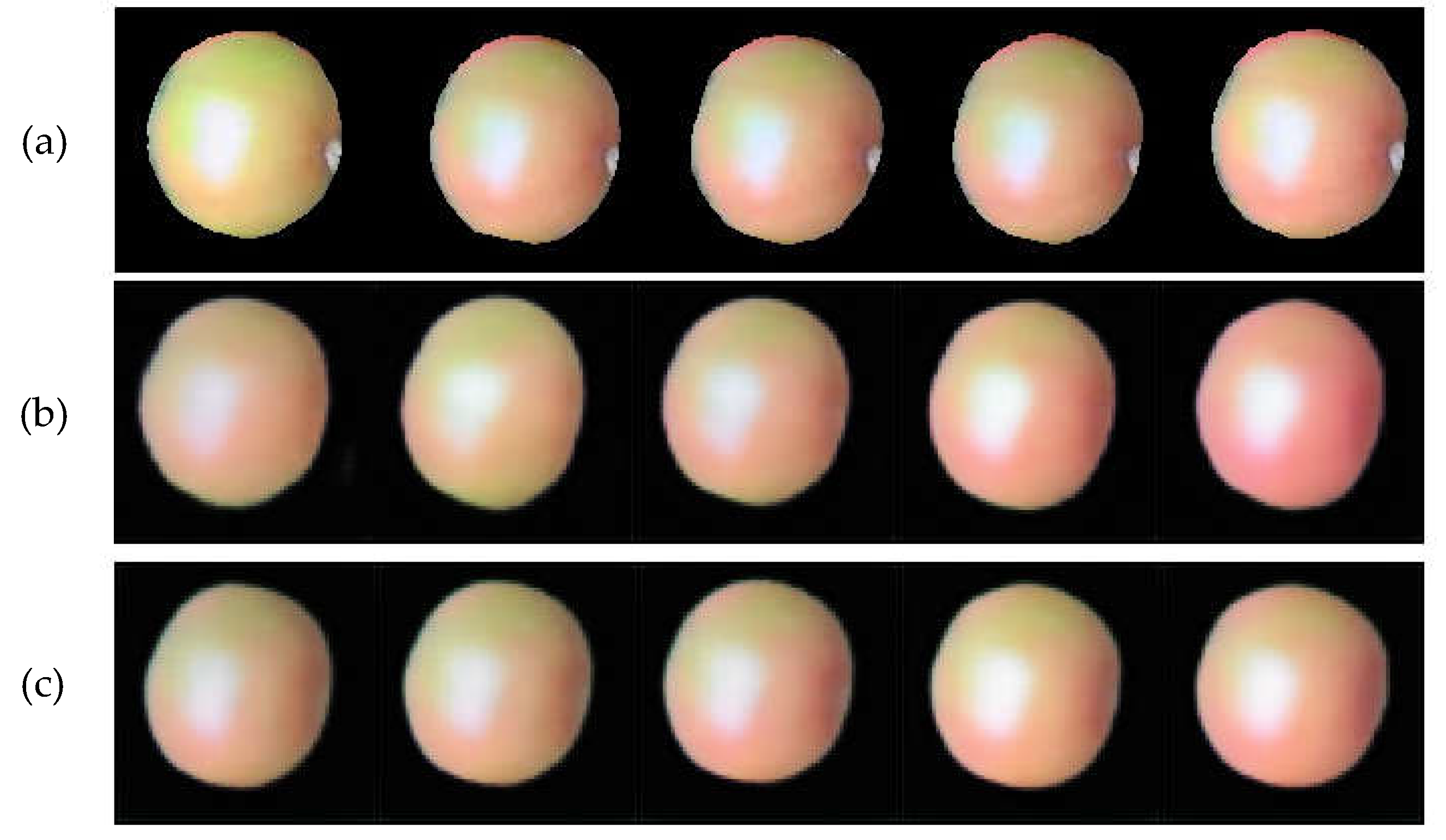
To select suitable prediction models for tomato growth, LSTM and GRU models of encoder-decoder structure are analyzed respectively. Compared with LSTM network structure, GRU uses an update gate to select and forget information at the same time, which improves the efficiency. Experimental results confirme that GRU network with encoder-decoder structure is more suitable for tomato fruit growth prediction during the color turning stage. Tomato growth prediction results are shown in
Figure 8. In terms of tomato shape prediction, the LSTM model of encoder decoder structure and the GRU model have similar prediction effect, and the GRU model is closer to the real tomato growth situation in terms of tomato color prediction.
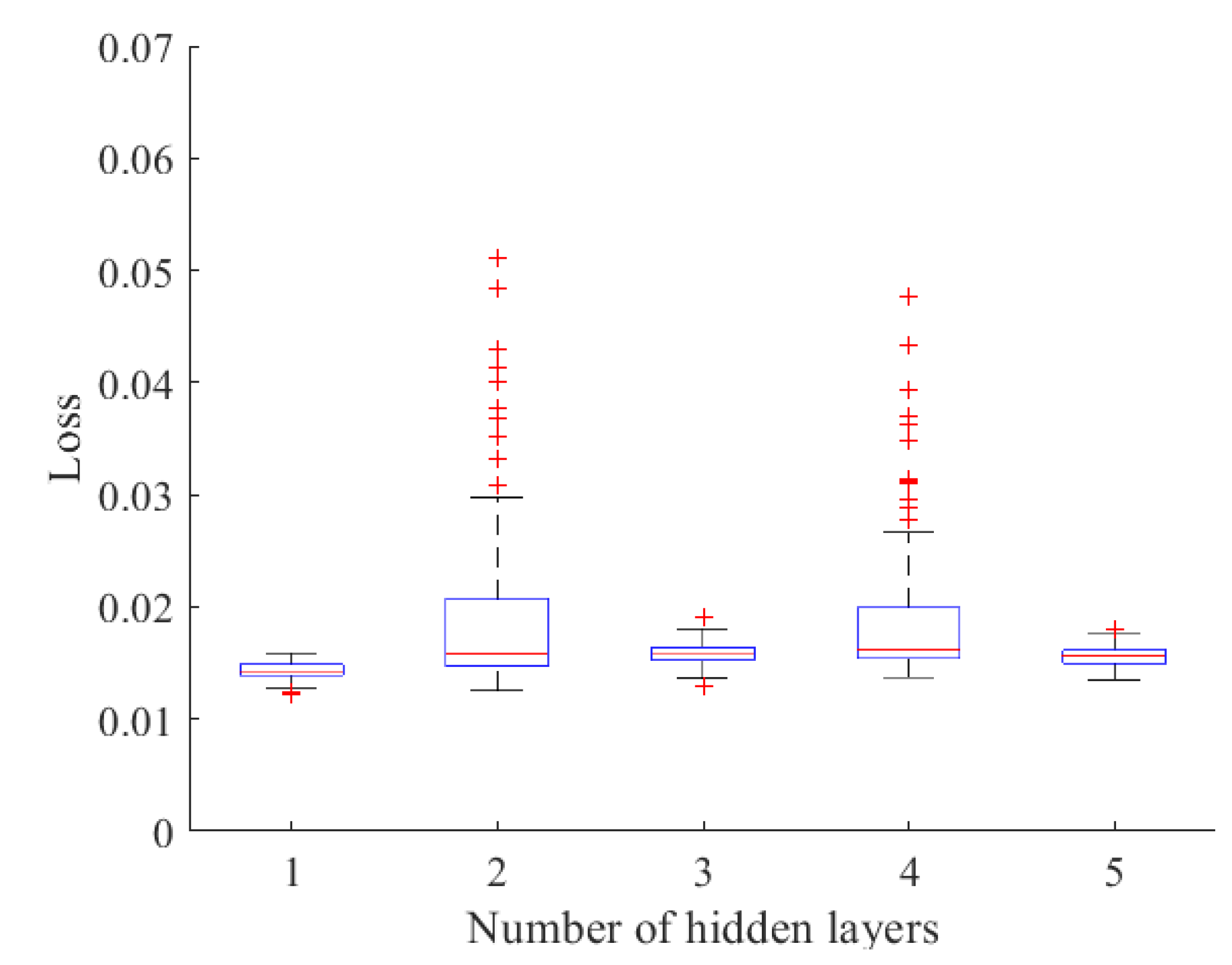
The number of hidden layers has a great impact on model performance. Therefore, the hidden layers of the network are set as 1,2,3,4,5,6 in this study. As shown in
Table 6, the model with odd number of hidden layers is better than the model with even number of hidden layers in predicting tomato growth color. As the number of network layers increases, the more difficult the model training will be, the more serious the overfitting will be, and the effect of shape and color prediction will become worse. In this study, the model with the least number of layers but the performance second only to the optimal performance is chosen as the hidden layer number 1.
Figure 9 shows the change curve of loss value in the last 100 rounds of training. When the number of hidden layers is 1, there are two specific points, both of which are low specific points, indicating that the loss value is lower than other loss values, and the loss value is small and the fluctuation range is small.
4.3.2. Influence of Different Network Structures on the Prediction Performance
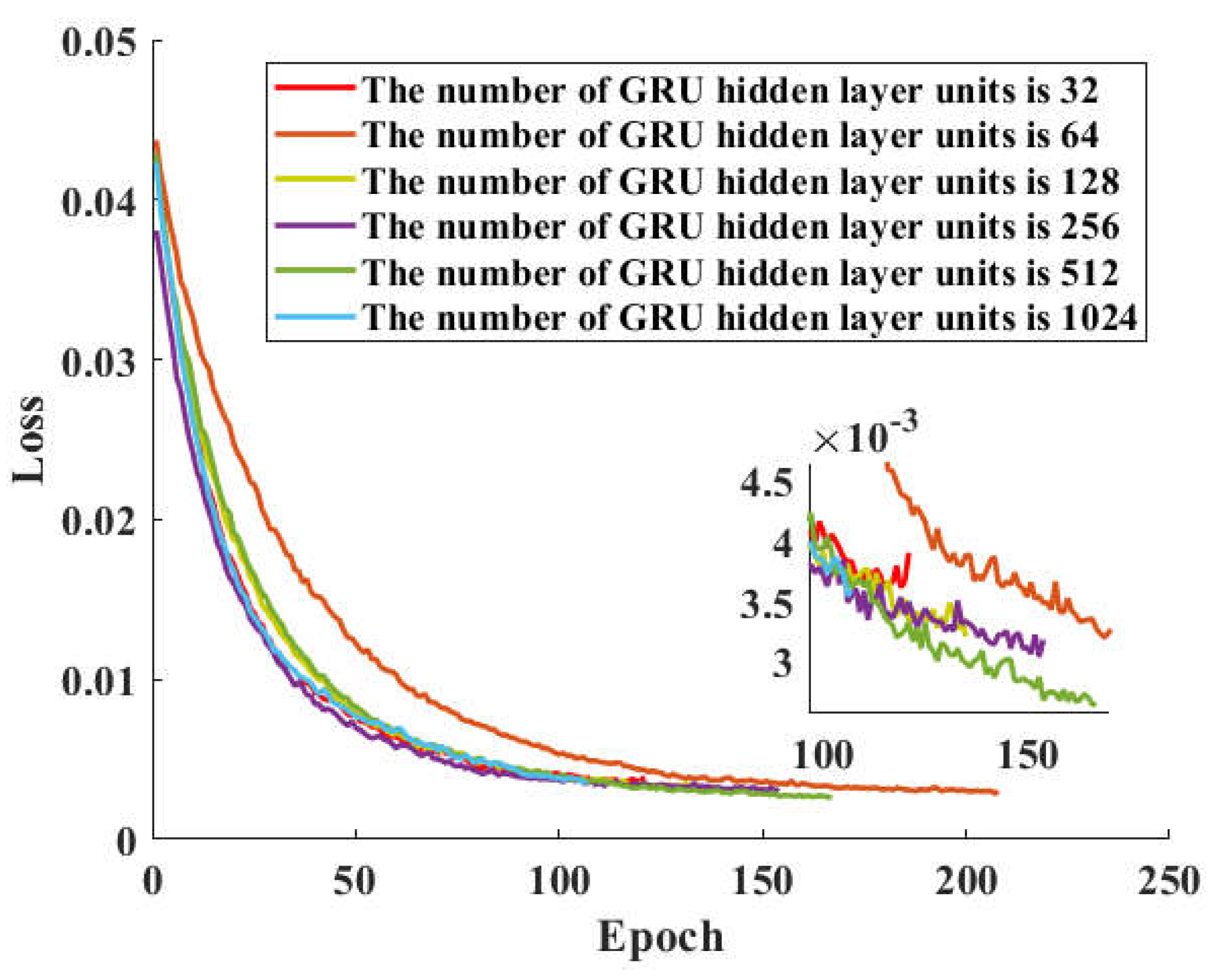
Parameter adjustment directly affects the performance of the model. In this study, the number of hidden layer units of the model is set as 32,64,128,256,512,1024, respectively. The loss function curve of the model is shown in
Figure 10. The number of hidden layer elements selected in this paper is 512. It can be seen from the loss curve that the model is easier to train and the loss value is the lowest after 100 rounds, and the model has the best convergence effect.
Table 7 shows the SSIM values of the model training real image and the predicted image under different elements of the hidden layer. When the number of elements of the hidden layer is set to 512, the SSIM value of 0.77 is the highest, indicating the best performance of the model. The predicted results of tomato growth trend have a high consistency with the actual growth trend of tomato. When the number of hidden layer elements is small, the ability of model to extract features is poor, and there is a large gap between the tomato growth prediction effect and the actual tomato growth. If the number of hidden layer elements is too large, the calculation cost and size of the model will be increased.
4.3.3. The influence of Environmental Conditions on the Prediction Performance
The tomato fruits mature in stages from bottom to top, so the greenhouse environment of fruits with different ripening times is slightly different. One spike, three spikes and five spikes are selected for color change prediction research. The color change date and corresponding environmental data of selected fruits are shown in
Table 8.
As can be seen from
Table 8, air temperature, light intensity and soil temperature are the major environmental differences between tomatoes with different ripening dates, while other environmental factors have no obvious differences and change rules. Temperature has an important influence on the growth and development of tomato. Low temperature is likely to lead to slow development and delayed fruit ripening, which has a great influence on its early maturity and high yield, and also affects the synthesis of lycopene. High temperature is likely to lead to premature plant aging, lower fruit setting rate and smaller fruit size [
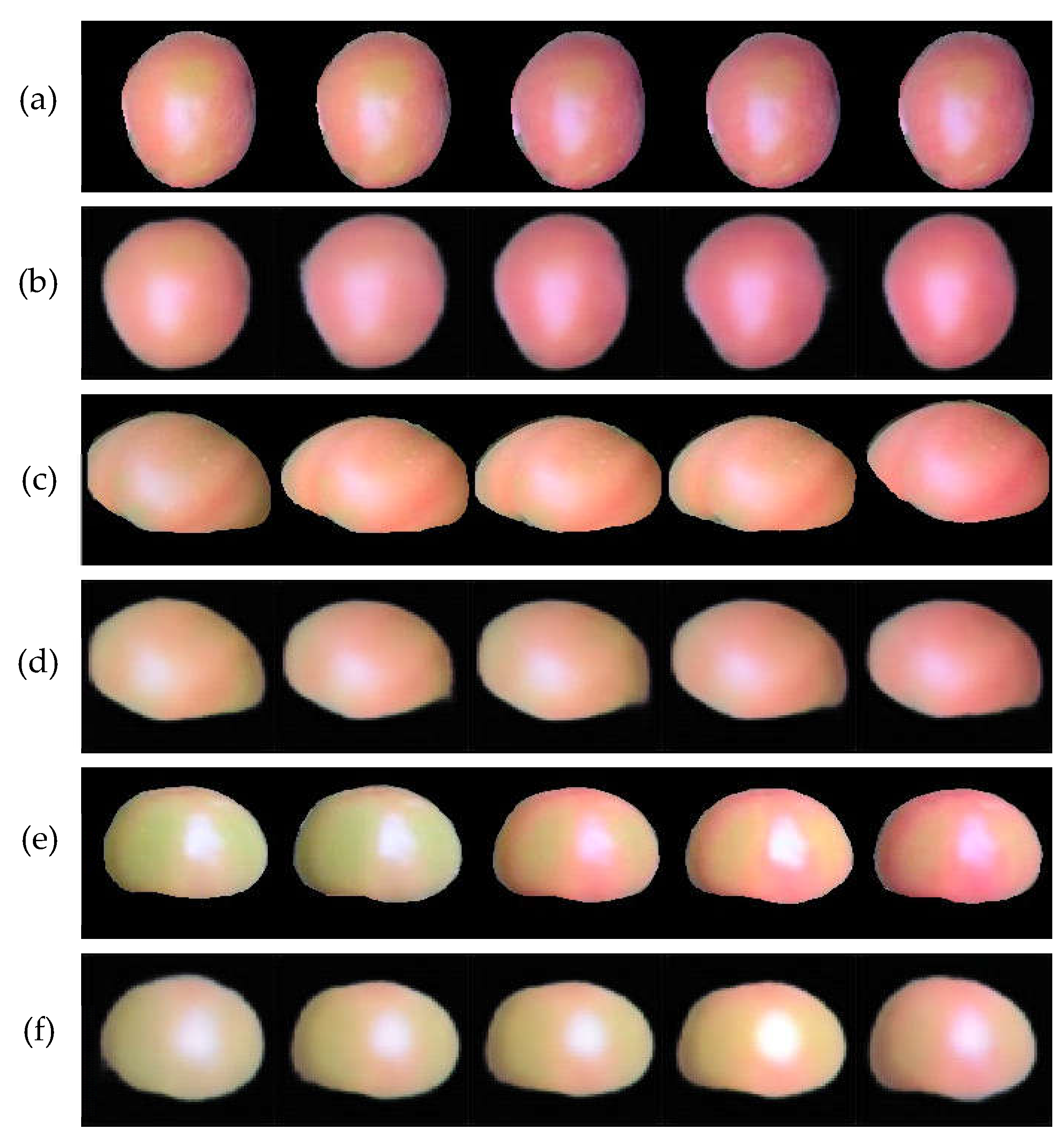
31]. The prediction results are shown in
Figure 11. Input t-4, t-3, t-2, t-1, t time to predict the growth of tomato at t+1, t+2, t+3, t+4, t+5 time. With the increase of temperature and light intensity, the color change time of tomato is shortened, and the time from green ripening stage to red ripening stage is about 10.5 days, 8.3 days and 7.1 days, which confirm that the greenhouse environment of five spikes is more suitable for the color change of tomato at maturity stage. When the greenhouse environment maintains a temperature at 24.93℃, light intensity at 11.26 Klux and soil temperature at 24.06℃, it is conducive to lycopene production, which aligns with the findings of Shamshiri et al. [
32].
5. Conclusion
Most of the phenotypic studies of plants focus on leaves or plants [
33], and the typical representative is Arabidopsis thaliana [
23]. It is of great guiding significance for agricultural development to study the breeding cycle of buildings through the growth trend of plants [
34]. The color and shape of tomato determine the nutritional and economic value of tomato entering the market. Tomato phenotype prediction is the most intuitive way to study the growth status of tomato, which can clearly observe the external morphological characteristics of tomato such as color and shape. There are relatively few studies on tomato fruit phenotype, and research on tomato phenotype prediction has important guiding significance for tomato growth.
Plant growth monitoring is a crucial approach for assessing environmental conditions, comprehending environmental information, and determining plant growth status [
35].The goal of this paper is to use the color and shape features of tomatoes on historical images to predict the future growth trend of tomatoes in color and shape, and construct a time-dependent relationship. The growth cycle of tomato fruit and the requirements of environmental conditions for tomato fruit growth can be studied.
The GRU network with encoder-decoder structure is used to predict the growth trend of tomato at multiple times in the future according to the growth state of tomato at historical times combined with greenhouse environment data. The experimental results show that the number of hidden layers and hidden layer units of the selected network meet the requirements. According to the SSIM index, the predicted results of tomato are highly similar to the true growth trend of tomato. In greenhouse environment, sensors are used to collect related environmental data, air temperature, light intensity and soil moisture are three factors that have great influence on its growth. The prediction results of tomato in greenhouse environment with different network structures, different number of hidden layers and different number of hidden layer units under the same network structure are discussed. The study of the future growth state of tomatoes in color and shape is consistent with the results of the study by Shamshiri et al. [
32].
In this paper, a GRU network with encoder-decoder structure combined with environmental data is proposed. The multi-step tomato growth prediction dataset based on time series data is used to predict the color and shape of the tomato combined with the historical state of the tomato. The tomato growth process was visualized, and the greenhouse tomato growth prediction results under different hidden layer numbers, hidden layer units and different environmental conditions were analyzed. The experimental results showed that the proposed model had a high consistency with the actual growth state of tomato, the SSIM was 0.746, the model had a good effect when the number of hidden layers was 1 and the number of hidden layer units was 512. It was proved that the average temperature was 24.93℃, the average soil temperature was 24.06℃, and the average light intensity was 11.26 Klux, which was the most suitable for tomato growth. Greenhouse environmental conditions such as average air humidity, average carbon dioxide concentration, average soil moisture and average soil concentration had little influence on the results of tomato prediction. The RGB three-channel image data, which was more intuitive, was utilized to analyze the impact of environmental conditions on tomato growth cycle. This paper provided a theoretical basis for investigating suitable greenhouse environmental conditions for tomato cultivation and accurate timing for harvesting. Furthermore, it offered theoretical and technical guidance for precise regulation and automatic management of tomato growth in solar greenhouses.
Author Contributions
Data curation, F.S. and T.L.; investigation, S.L.; methodology, Y.Z.; software,S.L.; supervision, T.L. and L.Z.; validation, L.Z. and S.C.; visualization, F.S. and S.C.; writing—original draft, S.L. and Y.Z.;writing—review and editing, S.L. and L.Z. All authors have read and agreed to the published versionof the manuscript.
Funding
This research was supported by the science and technology smes innovation ability improvement project of Shandong Province (2022TSGC2047), and the Major Science and Technology Innovation Project of Shandong Province (2022CXGC020708).
Institutional Review Board Statement
Not applicable.
Data Availability Statement
All data are presented in this article in the form of figures and tables.
Acknowledgments
The authors would like to thank the editors and all the reviewers who participated in the review.
Conflicts of Interest
The authors declare no conflict of interest.
References
- López-Correa, J.M.; Moreno, H.; Ribeiro, A. and Andújar, D. Intelligent Weed Management Based on Object Detection Neural Networks in Tomato Crops. Agronomy-Basel. 2022, 12, 2953. [Google Scholar] [CrossRef]
- Wang, X. and Liu, J. Tomato anomalies detection in greenhouse scenarios based on YOLO-Dense. Front. Plant. Sci. 2021, 12, 634103. [Google Scholar] [CrossRef]
- Nagase, K.; Shiraki, T. and Iwasaki, H. Plant factory solution with instrumentation and control technology. Fuji electric review. 2016, 62, 160–164. [Google Scholar]
- Chen, L.; Pan, Y.; Li, H.; Liu, Z.; Jia, X.; Li, W.; Jia, H. and Li, X. Constant temperature during postharvest storage delays fruit ripening and enhances the antioxidant capacity of mature green tomato. J. Food. Process. Pres. 2020, 44, e14831. [Google Scholar] [CrossRef]
- Li, N.; Wu, X.; Zhuang, W.; Xia, L.; Chen, Y.; Wu, C.; Rao, Z.; Du, L.; Zhao, R. and Yi, M. Tomato and lycopene and multiple health outcomes: Umbrella review. Food. Chem. 2021, 343, 128396. [Google Scholar] [CrossRef]
- Kaur, K. and Gupta, O. A machine learning approach to determine maturity stages of tomatoes. Orient. j. comput. sci. technol. 2017, 10, 683–690. [Google Scholar] [CrossRef]
- Arivazhagan, S.; Shebiah, R.N.; Nidhyanandhan, S.S. and Ganesan, L. Fruit recognition using color and texture features. J. emerg. trends. comput. inf. sci. 2010, 1, 90–94. [Google Scholar] [CrossRef]
- Bojacá, C.R.; Gil, R. and Cooman, A. Use of geostatistical and crop growth modelling to assess the variability of greenhouse tomato yield caused by spatial temperature variations. Comput. Electron. Agr. 2009, 65, 219–227. [Google Scholar] [CrossRef]
- Ghavami, M. Development of Internet of Things based smart multi-sensors system for early prediction of plant growth. Master of Science, University of Manitoba, Canada, 2022. http://hdl.handle.net/1993/36507.
- Kozukue, N. and Friedman, M. Tomatine, chlorophyll, β-carotene and lycopene content in tomatoes during growth and maturation. J. Sci. Food. Agric. 2003, 83, 195–200. [Google Scholar] [CrossRef]
- Barrett, D.M.; Beaulieu, J.C. and Shewfelt, R. Color, flavor, texture, and nutritional quality of fresh-cut fruits and vegetables: desirable levels, instrumental and sensory measurement, and the effects of processing. Crit. Rev. Food. Sci. 2010, 50, 369–389. [Google Scholar] [CrossRef]
- Sugino, N.; Watanabe, T. and Kitazawa, H. Effect of transportation temperature on tomato fruit quality: chilling injury and relationship between mass loss and a* values. J. Food. Meas. Charact. 2022, 16, 2884–2889. [Google Scholar] [CrossRef]
- Kuijpers, W.J.; van de Molengraft, M.; van Mourik, S.; van’t Ooster, A.; Hemming, S. and van Henten, E.J. Model selection with a common structure: Tomato crop growth models. Biosyst. Eng. 2019, 187, 247–257. [Google Scholar] [CrossRef]
- Samal, S.; Acharya, B. and Barik, P.K. Internet of Things (IoT) in agriculture toward urban greening. AI, Edge and IoT-based Smart Agriculture, Elsevier: 2022, pp. 171-182. [CrossRef]
- Ayaz, M.; Ammad-Uddin, M.; Sharif, Z.; Mansour, A. and Aggoune, E.H.M. Internet-of-Things (IoT)-based smart ag-riculture: Toward making the fields talk. IEEE. Access. 2019, 7, 129551–129583. [Google Scholar] [CrossRef]
- Ting, L.; Yuhan, J.; Man, Z.; Sha, S. and Minzan, L. Universality of an improved photosynthesis prediction model based on PSO-SVM at all growth stages of tomato. Int. J Agr. Biol. Eng. 2017, 10, 63–73. [Google Scholar] [CrossRef]
- Harun, A.N.; Mohamed, N.; Ahmad, R. and Ani, N.N. Improved Internet of Things (IoT) monitoring system for growth optimization of Brassica chinensis. Comput. Electron. Agr. 2019, 164, 104836. [Google Scholar] [CrossRef]
- Liao, M.S.; Chen, S.F.; Chou, C.Y.; Chen, H.Y.; Yeh, S.H.; Chang, Y.C. and Jiang, J.A. On precisely relating the growth of Phalaenopsis leaves to greenhouse environmental factors by using an IoT-based monitoring system. Comput. Electron. Agr. 2017, 136, 125–139. [Google Scholar] [CrossRef]
- Kocian, A.; Massa, D.; Cannazzaro, S.; Incrocci, L.; Di Lonardo, S.; Milazzo, P. and Chessa, S. Dynamic Bayesian network for crop growth prediction in greenhouses. Comput. Electron. Agr. 2020, 169, 105167. [Google Scholar] [CrossRef]
- Cisternas, I.; Velásquez, I.; Caro, A. and Rodríguez, A. Systematic literature review of implementations of precision agriculture. Comput. Electron. Agr. 2020, 176, 105626. [Google Scholar] [CrossRef]
- Del Borghi, A.; Tacchino, V.; Moreschi, L.; Matarazzo, A.; Gallo, M. and Vazquez, D.A. Environmental assessment of vegetable crops towards the water-energy-food nexus: A combination of precision agriculture and life cycle assessment. Ecol. Indic. 2022, 140, 109015. [Google Scholar] [CrossRef]
- Jiang, Z.; Liu, C.; Hendricks, N.P.; Ganapathysubramanian, B.; Hayes, D.J. and Sarkar, S. Predicting county level corn yields using deep long short term memory models. arXiv:1805.12044. [CrossRef]
- Yasrab, R.; Zhang, J.; Smyth, P. and Pound, M.P. Predicting plant growth from time-series data using deep learning. Remote. Sens-Basel. 2021, 13, 331. [Google Scholar] [CrossRef]
- Zhu, Q.; Chen, J.; Zhu, L.; Duan, X. and Liu, Y. Wind speed prediction with spatio–temporal correlation: A deep learning approach. Energies. 2018, 11, 705. [Google Scholar] [CrossRef]
- Zaremba, W.; Sutskever, I. and Vinyals, O. Recurrent neural network regularization. arXiv:1409.2329. [CrossRef]
- Bengio, Y.; Simard, P. and Frasconi, P. Learning long-term dependencies with gradient descent is difficult. IEEE. T. Neural. Networ. 1994, 5, 157–166. [Google Scholar] [CrossRef] [PubMed]
- Graves, A. Long short-term memory. Supervised sequence labelling with recurrent neural net-works. Springer link: 2012, 9, 37–45. [Google Scholar] [CrossRef]
- Wang, Z.; Li, Y.; Li, Z.; Zhao, C.; Gao, F. and Wang, P. Reduced-order DC terminal dynamic model for multi-port AC-DC power electronic transformer. Energies. 2019, 12, 2130. [Google Scholar] [CrossRef]
- Wang, Y.; Liao, W. and Chang, Y. Gated recurrent unit network-based short-term photovoltaic forecasting. Energies. 2018, 11, 2163. [Google Scholar] [CrossRef]
- Wang, Z. Applications of objective image quality assessment methods [applications corner]. IEEE. Signal. Proc. Mag. 2011, 28, 137–142. [Google Scholar] [CrossRef]
- Van Ploeg, D. and Heuvelink, E. Influence of sub-optimal temperature on tomato growth and yield: a review. J. Hortic. Sci. Biotech. 2005, 80, 652–659. [Google Scholar] [CrossRef]
- Shamshiri, R.R.; Jones, J.W.; Thorp, K.R.; Ahmad, D.; Man, H.C. and Taheri, S. Review of optimum temperature, humidity, and vapour pressure deficit for microclimate evaluation and control in greenhouse cultivation of tomato: a review. Int. agrophys. 2018, 32, 287–302. [Google Scholar] [CrossRef]
- Sakurai, S.; Uchiyama, H.; Shimada, A. and Taniguchi, R-i. Plant Growth Prediction using Convolutional LSTM. VISI-GRAPP. 2019, 5, 105–113. [Google Scholar] [CrossRef]
- Rizkiana, A.; Nugroho, A.; Salma, N.; Afif, S.; Masithoh, R.; Sutiarso, L. and Okayasu, T. Plant growth prediction model for lettuce (Lactuca sativa.) in plant factories using artificial neural network. IOP Conference Series: Earth and Environmental Science, Malang, Indonesia, 25 August 2020. [Google Scholar] [CrossRef]
- Okayasu, T.; Nugroho, A.P.; Sakai, A.; Arita, D.; Yoshinaga, T. ; Taniguchi, R-i.; Horimoto, M., Inoue, E., Eds.; Hirai, Y. and Mitsuoka, M. Affordable field environmental monitoring and plant growth measurement system for smart agriculture. IEEE: 2017 Eleventh International Conference on Sensing Technology (ICST), Sydney, Australia, 01 March 2018. [Google Scholar] [CrossRef]
Figure 1.
The system architecture of data acquisition.
Figure 1.
The system architecture of data acquisition.
Figure 2.
The stereogram layout of IoT sensors.
Figure 2.
The stereogram layout of IoT sensors.
Figure 3.
Strakes layout of sensors.
Figure 3.
Strakes layout of sensors.
Figure 4.
Tomato images. (a) The original tomato image. (b) The tomato image with removed background information.
Figure 4.
Tomato images. (a) The original tomato image. (b) The tomato image with removed background information.
Figure 5.
The encoder-decoder structure.
Figure 5.
The encoder-decoder structure.
Figure 6.
LSTM model with encoder-decoder structure.
Figure 6.
LSTM model with encoder-decoder structure.
Figure 7.
GRU model with encoder-decoder structure.
Figure 7.
GRU model with encoder-decoder structure.
Figure 8.
Tomato growth prediction results of LSTM and GRU models with encoder-decoder structure. (a) Real tomato images (b)LSTM tomato growth prediction results (c) GRU tomato growth prediction results.
Figure 8.
Tomato growth prediction results of LSTM and GRU models with encoder-decoder structure. (a) Real tomato images (b)LSTM tomato growth prediction results (c) GRU tomato growth prediction results.
Figure 9.
Loss values for the last 100 rounds.
Figure 9.
Loss values for the last 100 rounds.
Figure 10.
Comparison of loss function curves of GRU models with different number of hidden layer units in encoder-decoder structure.
Figure 10.
Comparison of loss function curves of GRU models with different number of hidden layer units in encoder-decoder structure.
Figure 11.
Prediction results of tomato color at different stages (environment), (a) real tomato images at five panicle (b) prediction results for tomato at five panicle (c) real tomato images at three panicle (d) prediction results for tomato at three panicle (e) real tomato images at the first panicle (f) prediction results for tomato at the first panicle.
Table 1.
Tomato growth cycle.
Table 1.
Tomato growth cycle.
| Growing stage |
Evidence of division |
Notes on agricultural management |
| Seedling stage |
Differentiation began from the emergence of the first true leaf to the third spike of flowers after planting |
To cultivate strong seedlings, adjust growth and good root system, prevent seedlings from growing or aging |
| Flowering and fruit setting stage |
From the appearance of flowers in the fourth ear to the fruit set in the first ear, the fruit reaches the size of walnut |
Vegetative growth and reproductive growth coexist, timely pruning, pollination, hanging vines, flower and fruit thinning |
| Fruit stage |
From the beginning of the first ear fruit of the tomato plant until the end of the seedlings |
Ensure that the tomato nutrition is sufficient in time to pick the heart, thin fruit, beat off the side branches |
Table 2.
Water and fertilizer management in the fruiting period.
Table 2.
Water and fertilizer management in the fruiting period.
| Water and fertilizer operation |
Number of irrigation |
Amount of irrigation |
Topdressing scheme management |
| Notes |
Flower-promoting water: drip irrigation is used to promote flower-promoting water about 25 days after planting |
Flower-promoting water: every 667 m3 of irrigation 6~8 m3
|
Fertilise 2~4 kg of NPK compound fertilizer (ratio: 10:40:10) + 0.25-0.5 kg of borax fertilizer every 667 with water |
Table 3.
Agricultural management in the fruiting period.
Table 3.
Agricultural management in the fruiting period.
| Farming operation |
Pruning |
Pollination |
Hanging vines |
Flower thinning |
Fruit thinning |
| Notes |
Remove the side branches under the first spike when they are about 5cm long. As the plant continues to grow, the branching process should be performed |
When the first spike has 2 or 3 flowers, the pollination operation is performed. When the petals of female flowers are fully expanded and extended to the shape of a trumpet, it is appropriate to pollination |
They are wound manually every 5 to 7 days to keep the main stem growing upward |
5~6 normal and robust flower buds are selected for each spike, and the rest are all drained. Defoliate the first earliest flower in the first spike |
Abnormal fruit and extra small fruit are thinned, and 3~4 fruit per ear are kept |
Table 4.
Parameters of environmental sensors.
Table 4.
Parameters of environmental sensors.
| Sensor |
Type |
Measuring range |
Precision |
Output signal |
| Air temperature and humidity sensor |
DB-171 |
Temperature: -40~120℃
Humidity: 0~100 %RH |
±0.1℃
±1.0% RH |
4-20 mA |
| CO2 sensor |
EE820 |
0~2000 PPM |
±50 PPM |
4-20 mA |
| Light sensor |
TBQ-6 |
0~200 Klux |
±0.02 Klux |
4-20 mA |
| Soil sensor |
5TE |
Temperature: -40~60℃
Humidity: 0~80% VWC
Electrical conductivity:0~23 dS/m |
±0.1℃
±0.08 %VWC
0.01 dS/m |
Digital signal |
Table 5.
LSTM and GRU model indexes of encoder decoder structure.
Table 5.
LSTM and GRU model indexes of encoder decoder structure.
| Model |
SSIM |
Model size/MB |
| LSTM |
0.738 |
141 |
| GRU |
0.746 |
111 |
Table 6.
SSIM index of different hidden layers in GRU model of encoder-decoder structure.
Table 6.
SSIM index of different hidden layers in GRU model of encoder-decoder structure.
| Number of hidden layers |
1 |
2 |
3 |
4 |
5 |
6 |
| SSIM |
0.76 |
0.63 |
0.72 |
0.68 |
0.77 |
0.70 |
Table 7.
SSIM index of number of units in different hidden layers for GRU model of encoder-decoder structure.
Table 7.
SSIM index of number of units in different hidden layers for GRU model of encoder-decoder structure.
| Number of hidden layer units |
32 |
64 |
128 |
256 |
512 |
1024 |
| SSIM |
0.698 |
0.697 |
0.693 |
0.728 |
0.770 |
0.690 |
Table 8.
LSTM and GRU model indexes of encoder decoder structure.
Table 8.
LSTM and GRU model indexes of encoder decoder structure.
| Fruit stage |
One spike |
Three spikes |
Five spikes |
| Color tuning stages |
5.9~5.19 |
6.3~6.11 |
6.20~6.27 |
| Mean air temperature/℃ |
18.85 |
22.71 |
24.93 |
| Mean air humidity/%RH |
67.26 |
66.06 |
65.81 |
| Average light intensity/Klux |
8.66 |
10.37 |
11.26 |
| Mean CO2 concentration/PPM |
489.78 |
466.37 |
471.76 |
| Mean soil temperature/℃ |
17.65 |
21.93 |
24.06 |
| Mean soil moisture/VWC |
26.21 |
26.96 |
26.46 |
| Average soil conductivity/dS/m |
0.68 |
0.67 |
0.72 |
|
Disclaimer/Publisher’s Note: The statements, opinions and data contained in all publications are solely those of the individual author(s) and contributor(s) and not of MDPI and/or the editor(s). MDPI and/or the editor(s) disclaim responsibility for any injury to people or property resulting from any ideas, methods, instructions or products referred to in the content. |
© 2024 by the authors. Licensee MDPI, Basel, Switzerland. This article is an open access article distributed under the terms and conditions of the Creative Commons Attribution (CC BY) license (http://creativecommons.org/licenses/by/4.0/).
