Insights into Psychiatric Diseases Represented by Wave Equations: A Mathematical and Graphical Exploration

Richard Montgomery

doi:10.20944/preprints202407.0090.v1

Submitted:

29 June 2024

Posted:

01 July 2024

You are already at the latest version

Abstract

Psychiatric disorders, characterized by complex and fluctuating patterns of thoughts, emotions, and behaviors, can be effectively modeled and visualized using mathematical wave equations. This study explores the representation of three major psychiatric conditions— Psychosis, Bipolar Disorder and Obsessive Compulsive Disorder (OCD)—through the application of differential equations, damping factors, and noise perturbations. Psychosis is modeled using Lissajous figures with high-frequency components, damping, and noise, symbolizing the irregular and erratic thought patterns characteristic of this condition. The inclusion of random perturbations and varying frequencies illustrates the chaotic and unpredictable nature of psychotic episodes, while damping effects reflect the temporary reductions in symptom intensity. For bipolar disorder, a system of partial differential equations simulates the cyclical nature of manic and depressive episodes. The model captures high-energy manic phases with periodic disturbances and the subsequent transition to lower-energy depressive states through damping effects. This representation highlights the oscillatory behavior and recurring episodes inherent to bipolar disorder. OCD is represented with Circumferential Complex Equations in Mult directions. The resulting graphical representations provide intuitive visual insights into the dynamics of these psychiatric disorders. By leveraging wave equations and mathematical modeling, this approach offers a novel perspective on understanding and analyzing the complex behaviors associated with OCD, bipolar disorder and psychosis. This method not only aids in the conceptualization of psychiatric phenomena but also underscores the potential of mathematical tools in the study of mental health conditions.

Keywords:

Keywords: Psychosis

;

Bipolar Disorder and Obsessive Compulsive Disorder

;

Simulation with waves and differential equations

Subject:

Biology and Life Sciences - Neuroscience and Neurology

Section 1. Introduction

Psychiatric disorders present some of the most intricate and challenging conditions to understand and treat due to their complex and dynamic nature. Recent advancements in computational psychiatry have introduced new methodologies to model and visualize these disorders, providing deeper insights into their underlying mechanisms. Among these methodologies, the application of wave equations offers a unique perspective on the fluctuating patterns of psychiatric symptoms.

Psychosis manifests through disorganized thoughts, delusions, and hallucinations. The irregular and erratic nature of psychotic episodes makes them particularly challenging to model. Recent studies have explored the role of neural oscillations and network disruptions in psychosis (Uhlhaas & Singer, 2015). By employing Lissajous figures and incorporating elements such as noise, damping, and varying frequencies, we can simulate the chaotic and unpredictable nature of psychosis, providing a visual and mathematical representation that aligns with clinical observations.

Bipolar disorder is characterized by alternating episodes of mania and depression, each exhibiting distinct energy levels, mood states, and behaviors. The cyclical nature of these episodes has been the focus of numerous studies, emphasizing the importance of understanding their oscillatory behavior (Geddes & Miklowitz, 2013). Traditional models often struggle to encapsulate the recurrent and dynamic aspects of bipolar disorder effectively. However, using partial differential equations (PDEs) to simulate these oscillations allows for a more nuanced representation of the disorder’s temporal dynamics.

Obsessive-compulsive disorder (OCD) is a chronic psychiatric condition characterized by persistent, intrusive thoughts (obsessions) and repetitive behaviors (compulsions). These symptoms often cause significant distress and impairment in daily functioning. The persistent nature of OCD symptoms and their tendency to shift focus from one obsession or compulsion to another make it a particularly challenging disorder to understand and treat.

To model the dynamics of OCD, we use spherical damped waves with orthogonal axis transformations. This mathematical approach captures the cyclical and recurring nature of OCD symptoms. The spherical damped wave equation represents the persistence of obsessions and compulsions, while the damping factor simulates the gradual reduction in symptom intensity over time. However, before the amplitude reaches zero, the wave regenerates along a new axis, symbolizing the migration of symptoms to a different focus.

This study aims to explore the use of wave equations to model and visualize the dynamics of bipolar disorder and psychosis. By leveraging the mathematical properties of waves, we can create intuitive, creative and informative graphical representations of these psychiatric conditions. This approach not only enhances our understanding of the disorders but also highlights the potential of mathematical modeling in psychiatric research.

Section 2. Methodology

Section 2.1 Psychosis

Equations Used in the Model

Time-Dependent Frequencies

\begin{array}{r} (1) & a (t) = a (1 + 0.1 t) \\ (2) & b (t) = b (1 + 0.1 t) \end{array}

where

a

and

b

are the initial frequencies, and

t

is the time variable.

2.: Damping Function

D (t) = e^{- 0.1 t}

3.: Noise Functions

\begin{array}{r} (3) & N_{x} (t) = 0.1 \cdot N (0,1) \\ (4) & N_{y} (t) = 0.1 \cdot N (0,1) \end{array}

where

N (0,1)

represents a normally distributed random variable.

4.: Lissajous Figures with Noise, Damping, and Acceleration

\begin{matrix} x (t) = A s i n (a (t) t + δ) D (t) + N_{x} (t) \\ y (t) = B s i n (b (t) t) D (t) + N_{y} (t) \end{matrix}

where

A

and

B

are the amplitudes,

δ

is the phase shift,

D (t)

is the damping function, and

N_{x} (t)

and

N_{y} (t)

are the noise functions.

Section 2.2 Representation of Bipolar Disorder

The model and the resulting graphical representation illustrate key aspects of bipolar disorder through the behavior of damped waves and periodic disturbances. Here’s why this model is an appropriate representation:

1.: Mania Phase

In bipolar disorder, the mania phase is characterized by elevated mood, increased energy, and heightened activity. This phase can be represented by:

\frac{d x}{d t} = A s i n (k t) e^{- α t}

High Amplitude and Energy: The sine function $s i n (k t)$ initially has high amplitude, representing the high energy and activity levels during mania.
Periodic Disturbances: The periodic nature of the sine function captures the cyclical nature of manic episodes.
Damping Factor: The exponential term $e^{- α t}$ introduces a damping effect, reflecting the fact that manic episodes do not last indefinitely and tend to decrease in intensity over time.

2.: Dispersion and Transition

The transition between mania and depression can be seen in the dispersion phase:

\frac{d y}{d t} = A s i n (ω t) e^{- α t}

Transition Phase: The sine function $s i n (ω t)$ on a different axis ( $y$ -axis) represents the transition phase where the individual moves from mania towards depression.
Dispersion Effect: The model disperses the energy along a new axis, symbolizing the shift in behavior and mood as the manic energy dissipates.

3.: Depression Phase

In bipolar disorder, the depression phase is marked by low energy, decreased activity, and feelings of sadness or hopelessness. This phase is modeled by the damping effects and decreasing amplitude over time:

◻

\begin{array}{r} (5) & x (t) = \int_{0}^{t} A s i n (k τ) e^{- α τ} d τ \\ (6) & y (t) = \int_{0}^{t} A s i n (ω τ) e^{- α τ} d τ \end{array}

Damping Over Time: The damping factor $e^{- α t}$ ensures that both $x (t)$ and $y (t)$ decrease over time, mirroring the decline in energy and activity during the depression phase.
Lower Amplitude: As time progresses, the amplitude of the waves decreases, reflecting the reduced activity and low energy levels characteristic of depression.

4.: Cyclical Nature

Bipolar disorder is known for its cyclical pattern of mood changes. The model captures this cyclical nature through the periodic functions and phase shifts:

Phase Shifts: The phase shifts $ϕ_{i}$ for each cycle represent the periodic recurrence of manic and depressive episodes.
Repetition: The system goes through multiple cycles, representing the recurring nature of bipolar disorder, where individuals experience multiple episodes of mania and depression.

Summary

The equations and their graphical representation effectively capture the key characteristics of bipolar disorder:

Mania Phase: High energy and activity, periodic disturbances.
Transition Phase: Dispersion and shift in behavior.
Depression Phase: Low energy, decreased activity, damping effects.
Cyclical Nature: Recurrence of manic and depressive episodes.

By modeling these aspects using damped waves, periodic functions, and phase shifts, the system provides a mathematical and visual representation of the complex and cyclical nature of bipolar disorder.

Section 2.3 Obsessive Compulsive Disorder (OCD)

1.: Initial Spherical Damped Wave Equation

The spherical wave equation with damping is given by:

r (t) = A e^{- α t} s i n (t + ϕ_{i})

where:

$A$ is the initial amplitude.
$α$ is the damping factor.
$t$ is the time variable.
$ϕ_{i}$ is the phase shift for the $i$ -th cycle.

2.: Propagation along Different Axes

For each cycle, the wave propagates along different axes. The coordinates for each axis are given by: Cycle

1 (i \equiv 0 (m o d 3))

: Propagation along the

x

and

y

axes.

\begin{matrix} (7) x (t) = r (t) s i n (t) \\ (8) y (t) = r (t) c o s (t) \\ z (t) = 0 \end{matrix}

Cycle

2 (i \equiv 1 (m o d 3))

: Propagation along the

y

and

z

axes.

\begin{array}{c} x (t) = 0 \\ (9) y (t) = r (t) s i n (t) \\ (10) z (t) = r (t) c o s (t) \end{array}

Cycle

3 (i \equiv 2 (m o d 3))

: Propagation along the

x

and

z

axes.

\begin{matrix} x (t) = r (t) c o s (t) \\ y (t) = 0 \\ z (t) = r (t) s i n (t) \end{matrix}

3.: Phase Shift for Each Cycle

The phase shift for the

i

-th cycle is given by:

ϕ_{i} = i \frac{π}{3}

where

i

ranges from 0 to

n - 1

(in this case,

n = 6

).

Summary of Transformations

For each cycle

i

:

1.: Calculate the radial distance $r (t)$ using equation (1) with the appropriate phase shift $ϕ_{i}$ .

2.: Apply the transformations to the coordinates $x (t), y (t)$ , and $z (t)$ based on the cycle number modulo 3, using equations (7)-(10).

Full Set of Equations

Combining the above, the full set of equations governing the OCD simulation for

n

cycles is:

r (t) = A e^{- α t} s i n (t + i \frac{π}{3})

For

i \equiv 0 (m o d 3)

:

\begin{matrix} x (t) = r (t) s i n (t) \\ y (t) = r (t) c o s (t) \\ z (t) = 0 \end{matrix}

For

i \equiv 1 (m o d 3)

:

\begin{matrix} x (t) = 0 \\ (11) y (t) = r (t) s i n (t) \\ (12) z (t) = r (t) c o s (t) \end{matrix}

For

i \equiv 2 (m o d 3)

:

\begin{matrix} x (t) = r (t) c o s (t) \\ y (t) = 0 \\ z (t) = r (t) s i n (t) \end{matrix}

Phase Shift

ϕ_{i} = i \frac{π}{3}

Section 3. Results

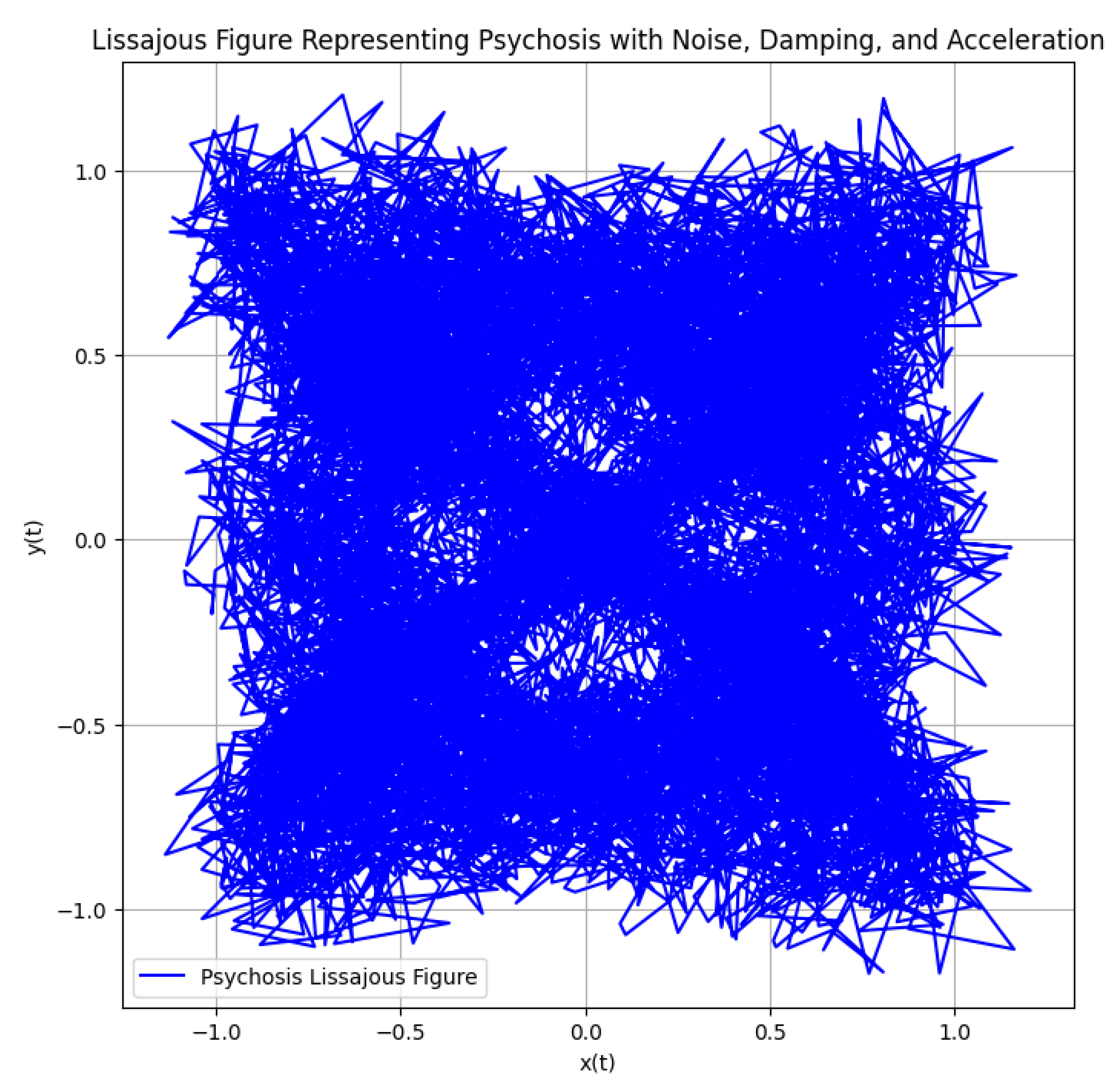
Figure 1. Chaotic representation of Psychosis with detachment from reality or an “anchor” support.

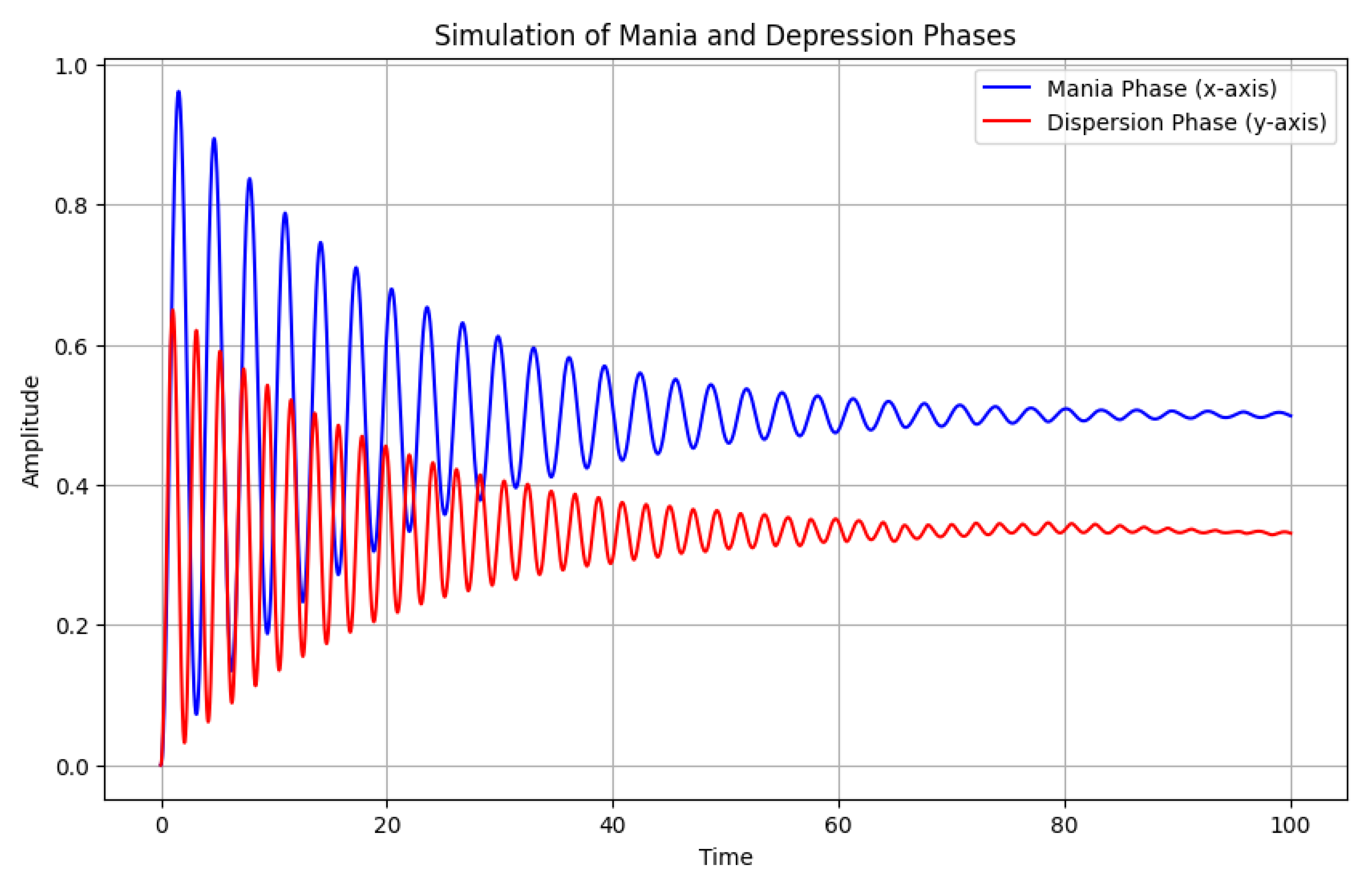
Figure 2. Bipolar Disorder represented, not in time scale, ups and downs and it reaches normalcy and recommences again.

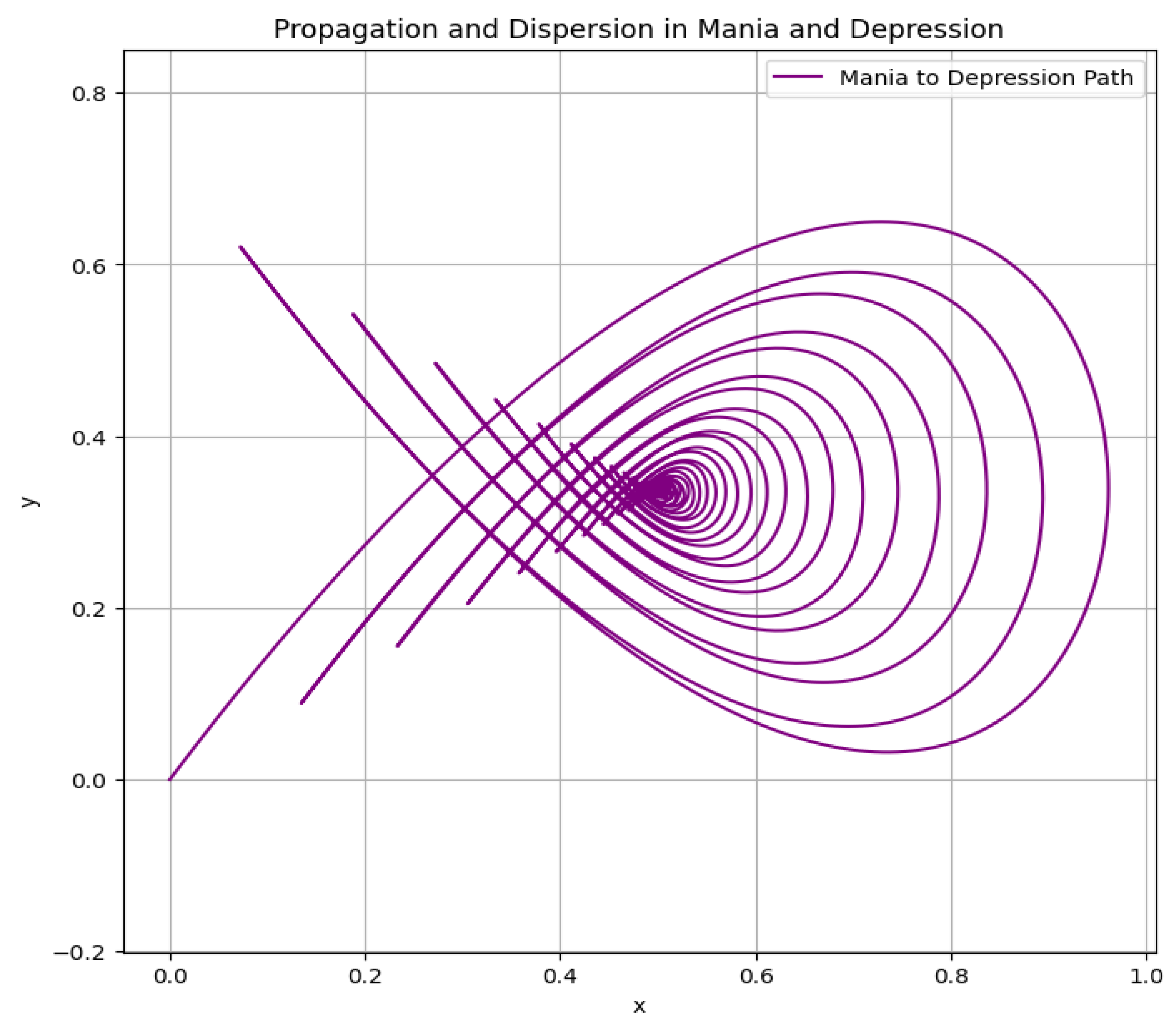
Figure 3. The same method of graph 2, but with an impression of infinity.

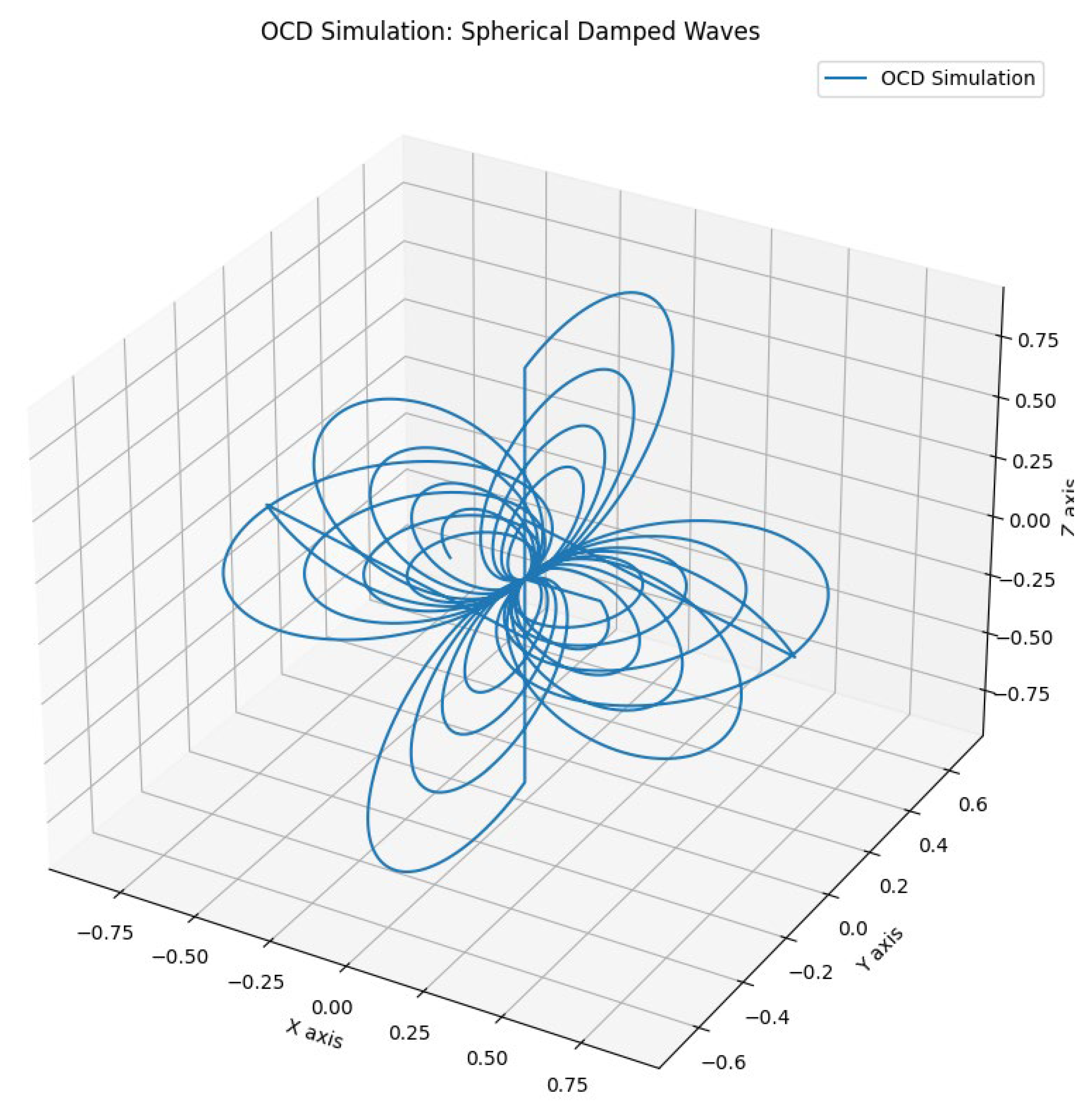
Figure 4. Multiaxial representation of OCD during life migrating from one group of symptoms to another, the natural path of the disease,.

Section 4. Discussion

Section 4. Modeling Psychosis Using Wave Equations

The three models presented in this study offer novel approaches to visualizing and understanding the complex nature of psychosis through the lens of mathematical wave equations. By incorporating elements such as noise, damping, and varying frequencies, these models provide insights into the erratic and unpredictable nature of psychotic episodes.

Irregular and Erratic Behaviour

Psychosis is characterized by disorganized thoughts, hallucinations, and delusions, which often manifest unpredictably and irregularly. The introduction of noise in our models simulates this randomness. These perturbations mimic the chaotic and disorganized nature of thought processes during psychosis, aligning with findings from studies on neural network disruptions in psychosis (Uhlhaas & Singer, 2015).

High Frequency and Intensity

Psychotic episodes often involve heightened sensory experiences and rapid thought processes. The high initial frequencies used in the models reflect this increased intensity. These high-frequency components capture the intense and fast-paced nature of psychotic symptoms, consistent with clinical observations that describe psychosis as a state of heightened arousal and sensory overload (Van der Stelt & Belger, 2007).

Damping and Acceleration Effects

Psychotic episodes are not static; their intensity can fluctuate over time. The damping factor and the time-dependent frequencies in the models illustrate these fluctuations. The damping factor represents the gradual reduction in symptom intensity, simulating periods where psychotic symptoms might temporarily decrease. Meanwhile, the varying frequencies simulate the acceleration effect, where the intensity of symptoms can increase rapidly, aligning with studies that highlight the fluctuating nature of psychotic experiences (Howes & Murray, 2014).

Complex Pathways and Disordered Patterns

The graphical representation of psychosis using Lissajous figures with noise, damping, and varying frequencies shows complex, non-repeating pathways, symbolizing the disorganized and fragmented thoughts experienced during psychosis. This intricate pattern reflects the multifaceted and unpredictable nature of psychotic episodes, capturing the essence of the disorder’s symptomatic diversity. This aligns with the conceptual framework that views psychosis as a disruption in the brain’s normal oscillatory activity, leading to altered perception and cognition (Uhlhaas & Singer, 2015) of the reality.

Some if my previous articles about circuit, and network heterogeneity in brain abnormalities provides a framework for understanding the individual variability within common functional networks in psychosis (Montgomery, 2024). The works emphasizes the importance of considering both common and individual-specific deviations in brain connectivity, which supports our model’s approach of incorporating noise and varying frequencies to simulate the erratic nature of psychosis.

Section 4.1 Modeling Bipolar Disorder Using Wave Equations

The second set of models employs partial differential equations to simulate the cyclical nature of bipolar disorder. By incorporating elements such as periodic disturbances and damping, these models capture the oscillatory behavior characteristic of manic and depressive episodes in bipolar disorder.

High Energy and Activity during Mania

Bipolar disorder is generally typified by episodes of mania, characterized by elevated mood, increased energy, and heightened activity levels. The initial high amplitude in our models represents this intense phase. Studies have shown that during manic episodes, individuals exhibit significantly higher levels of activity and energy (Grande et al., 2016). The wave equations reflect this by starting with a high amplitude, simulating the burst of energy experienced during mania, though we know not all bipolar patients behave like that.

Transition and Dispersion

The transition from mania to depression is a critical aspect of bipolar disorder. This phase is marked by a shift in mood and energy levels. In our models, this transition is represented by the dispersion effect, where the energy dissipates along a different axis. The differential equations incorporate periodic disturbances to simulate these shifts, aligning with findings that suggest bipolar disorder involves significant fluctuations in mood and energy (Judd et al., 2002).

Decreasing Amplitude in Depression

Depressive episodes in bipolar disorder are characterized by low energy, decreased activity, and feelings of sadness or hopelessness. This phase is modeled by the damping effects in our equations, which cause the amplitude to decrease over time. This reflects the gradual reduction in energy and activity levels, consistent with clinical observations of depressive episodes (Fagiolini et al., 2013).

Cyclical Nature and Recurrence

Bipolar disorder is known for its cyclical nature, with individuals experiencing repeated episodes of mania and depression. The periodic nature of the wave equations captures this cyclical pattern. Each cycle in the model represents a full oscillation from mania to depression and back, illustrating the recurring nature of the disorder. This is supported by literature indicating the chronic and recurrent course of bipolar disorder (Goodwin & Jamison, 2007).

Intuitive Visualization

The graphical representation of the models provides an intuitive visualization of the dynamics of bipolar disorder. The oscillating wave patterns clearly illustrate the transition from high-energy manic states to low-energy depressive states and back again. This visualization aligns with the conceptual framework of bipolar disorder as a condition involving significant mood swings and energy fluctuations (Miklowitz & Johnson, 2006).

Some of my research on brain network heterogeneity in psychiatric disorders underscores the importance of understanding individual variations within common functional circuits (Montgomery, 2024). My work on the multiscale characterization of gray matter volume differences across psychiatric conditions provides a deeper insight into the neural underpinnings of mood disorders, including bipolar disorder. This complements our approach by highlighting the complex and individualized nature of psychiatric conditions, further supporting the need for dynamic models to capture these nuances.

Section 4.3 Modeling OCD Using Spherical Damped Waves

The third model in this study uses spherical damped waves with orthogonal axis transformations to represent the persistent and cyclical nature of obsessive-compulsive disorder (OCD). This model captures the recurrence and shifting focus of obsessive-compulsive behaviours, which do not simply disappear but migrate to different areas (Graphic 3).

Persistent Nature of OCD

OCD is characterized by intrusive thoughts (obsessions) and repetitive behaviours (compulsions) that persist over time. The damped spherical wave equation in our model represents this persistence. Despite the damping effect, the wave regenerates before reaching zero amplitude, symbolizing the continuous presence of OCD symptoms. This aligns with clinical observations that OCD symptoms often persist and fluctuate in intensity rather than completely resolving (Abramowitz et al., 2009).

Migration and Shifting Focus

One of the defining features of OCD is the shifting focus of obsessions and compulsions. Patients may experience relief from one type of obsession or compulsion only to develop another. The orthogonal transformations in our model simulate this migration. After each cycle, the wave regenerates along a new axis, representing how OCD symptoms can shift in focus. This is consistent with findings that suggest OCD often involves changing themes and manifestations over time (Mataix-Cols et al., 2002).

Cyclical and Recurrent Nature

OCD is known for its cyclical and recurrent nature, where symptoms can worsen, improve, and then reappear. The model’s use of multiple cycles illustrates this recurrence. Each cycle shows the damped wave regenerating, simulating the recurrent nature of OCD where symptoms can diminish but then resurface in a different form. This cyclical pattern is well-documented in the literature, emphasizing the chronic and relapsing course of OCD (Siev & Steketee, 2010).

Complex and Disordered Patterns

The graphical representation of OCD using spherical waves with noise and damping creates complex, non-repetitive paths. These paths reflect the disorganized and often overwhelming experience of OCD, where intrusive thoughts and compulsive behaviours can feel uncontrollable and multifaceted. This aligns with the conceptual understanding of OCD as a disorder involving complex cognitive and behavioural patterns (Stein et al., 2019).

The use of spherical damped waves with orthogonal axis transformations provides a powerful model for understanding the dynamics of OCD. This approach captures the persistent, migratory, and recurrent nature of the disorder. By visualizing OCD symptoms as complex, regenerating waves, this model offers valuable insights into the chronic and fluctuating course of OCD, consistent with clinical observations and recent research findings.

Section 5. Conclusions

This study demonstrates the power of mathematical modeling in providing insights into the dynamics of psychiatric disorders. By employing wave equations, we have successfully captured the complex behaviors associated with bipolar disorder, psychosis, and obsessive-compulsive disorder (OCD).

For bipolar disorder, the use of partial differential equations effectively simulates the oscillatory nature of manic and depressive episodes. High initial amplitudes reflect the intense energy during mania, while damping effects illustrate the gradual decline into depression. The periodic nature of the model underscores the cyclical and recurrent nature of the disorder, aligning with clinical observations.

In modeling psychosis, the introduction of noise, high frequencies, and varying damping factors captures the erratic, intense, and fluctuating nature of psychotic episodes. The complex pathways generated in the Lissajous figures represent the disorganized thoughts and perceptions characteristic of psychosis. This approach provides a visual and mathematical representation that is consistent with current research on the neural oscillatory disruptions seen in psychotic disorders.

Overall, the use of wave equations to model these psychiatric disorders offers a novel perspective that enhances our understanding of their dynamic and complex nature. By providing intuitive graphical representations, these models serve as valuable tools for both clinical and research applications, offering deeper insights into the mechanisms underlying psychosis, bipolar disorder and OCD.

The use of spherical damped waves with orthogonal axis transformations provides a powerful model for understanding the dynamics of OCD. This approach captures the persistent, migratory, and recurrent nature of the disorder. By visualizing OCD symptoms as complex, regenerating waves, this model offers valuable insights into the chronic and fluctuating course of OCD, consistent with clinical observations and recent research findings.

This study demonstrates the power of mathematical modeling in providing insights into the dynamics of psychiatric disorders. By employing wave equations, we have successfully captured the complex behaviors associated with bipolar disorder, psychosis, and obsessive-compulsive disorder (OCD).

Overall, the use of wave equations to model these psychiatric disorders offers a novel perspective that enhances our understanding of their dynamic and complex nature. By providing intuitive graphical representations, these models serve as valuable tools for both clinical and research applications, offering deeper insights into the mechanisms underlying bipolar disorder, psychosis, and OCD.

Section 6. Attachments

Python Code: First Graph

import numpy as np

import matplotlib.pyplot as plt

# Parameters

A = 1

B = 1

a = 30 # High frequency

b = 20 # High frequency

delta = np.pi / 2

# Time variable

t = np.linspace(0, 2 * np.pi, 10000)

# Noise

noise_x = 0.1 * np.random.normal(size=t.shape)

noise_y = 0.1 * np.random.normal(size=t.shape)

# Damping

damping = np.exp(-0.1 * t)

# Acceleration (varying frequency)

a_t = a * (1 + 0.1 * t)

b_t = b * (1 + 0.1 * t)

# Lissajous figures with noise, damping, and acceleration

x = A * np.sin(a_t * t + delta) * damping + noise_x

y = B * np.sin(b_t * t) * damping + noise_y

# Plot

plt.figure(figsize=(8, 8))

plt.plot(x, y, label=‘Psychosis Lissajous Figure’, color=‘blue’)

plt.title(‘Lissajous Figure Representing Psychosis with Noise, Damping, and Acceleration’)

plt.xlabel(‘x(t)’)

plt.ylabel(‘y(t)’)

plt.legend()

plt.grid(True)

plt.axis(‘equal’)

plt.show()

Python Code: Second and Third Graph

Python Code fourth Graph.

import numpy as np

import matplotlib.pyplot as plt

from mpl_toolkits.mplot3d import Axes3D

# Parameters

A = 1 # Initial amplitude

damping_factor = 0.1 # Damping factor

num_cycles = 6 # Number of cycles

# Time variable

t = np.linspace(0, 4 * np.pi, 1000)

# Initialize arrays for storing the coordinates

x = []

y = []

z = []

# Function to generate damped spherical wave

def damped_spherical_wave(t, phase_shift):

r = A * np.exp(-damping_factor * t) * np.sin(t + phase_shift)

return r

# Generate the wave in different axes

for i in range(num_cycles):

phase_shift = i * np.pi / 3 # Phase shift for each cycle

if i % 3 == 0:

r = damped_spherical_wave(t, phase_shift)

x.extend(r * np.sin(t))

y.extend(r * np.cos(t))

z.extend(np.zeros_like(t))

elif i % 3 == 1:

r = damped_spherical_wave(t, phase_shift)

x.extend(np.zeros_like(t))

y.extend(r * np.sin(t))

z.extend(r * np.cos(t))

elif i % 3 == 2:

r = damped_spherical_wave(t, phase_shift)

x.extend(r * np.cos(t))

y.extend(np.zeros_like(t))

z.extend(r * np.sin(t))

# Plot the 3D wave

fig = plt.figure(figsize=(10, 10))

ax = fig.add_subplot(111, projection=‘3d’)

ax.plot(x, y, z, label=‘OCD Simulation’)

ax.set_title(‘OCD Simulation: Spherical Damped Waves’)

ax.set_xlabel(‘X axis’)

ax.set_ylabel(‘Y axis’)

ax.set_zlabel(‘Z axis’)

ax.legend()

plt.show()

References

Abramowitz, J. S., Taylor, S., & McKay, D. (2009). Obsessive-compulsive disorder. The Lancet, 374(9688), 491-499.
Geddes, J. R., & Miklowitz, D. J. (2013). Treatment of bipolar disorder. The Lancet, 381(9878), 1672-1682.
Grande, I., Berk, M., Birmaher, B., & Vieta, E. (2016). Bipolar disorder. The Lancet, 387(10027), 1561-1572.
Judd, L. L., Akiskal, H. S., Schettler, P. J., Endicott, J., Maser, J. D., Solomon, D. A., Leon, A. C., Coryell, W., Keller, M. B. (2002). The long-term natural history of the weekly symptomatic status of bipolar I disorder. Archives of General Psychiatry, 59(6), 530-537.
Mataix-Cols, D., do Rosario-Campos, M. C., & Leckman, J. F. (2005). A multidimensional model of obsessive-compulsive disorder. American Journal of Psychiatry, 162(2), 228-238.
Miklowitz, D. J., & Johnson, S. L. (2006). The psychopathology and treatment of bipolar disorder. Annual Review of Clinical Psychology, 2, 199-235.
Montgomery, R. M. (2024). Exploring Altered Neural Connectivity in Autism Spectrum Disorder: A Simulation of Spatial and Topological Proximities. TechRxiv.
Montgomery, R. M. (2024). Regional, circuit, and network heterogeneity of brain abnormalities in psychiatric disorders. Sciety.
Siev, J., & Steketee, G. (2010). Fears, beliefs, and rituals: Cognitive-behavioral treatment of obsessive-compulsive disorder. Oxford University Press.
Stein, D. J., Costa, D. L. C., Lochner, C., Miguel, E. C., Reddy, Y. C. J., Shavitt, R. G., & Van den Heuvel, O. A. (2019). Obsessive-compulsive disorder. Nature Reviews Disease Primers, 5(1), 52.
Uhlhaas, P. J., & Singer, W. (2015). Oscillatory activity and neuropsychiatric disorders: The role of inhibitory dysfunction and impaired temporal dynamics. Trends in Cognitive Sciences, 19(1), 42-51.

Disclaimer/Publisher’s Note: The statements, opinions and data contained in all publications are solely those of the individual author(s) and contributor(s) and not of MDPI and/or the editor(s). MDPI and/or the editor(s) disclaim responsibility for any injury to people or property resulting from any ideas, methods, instructions or products referred to in the content.

© 2024 by the authors. Licensee MDPI, Basel, Switzerland. This article is an open access article distributed under the terms and conditions of the Creative Commons Attribution (CC BY) license (http://creativecommons.org/licenses/by/4.0/).

Copyright: This open access article is published under a Creative Commons CC BY 4.0 license, which permit the free download, distribution, and reuse, provided that the author and preprint are cited in any reuse.

Insights into Psychiatric Diseases Represented by Wave Equations: A Mathematical and Graphical Exploration

Abstract

Keywords:

Subject:

Section 1. Introduction

Section 2. Methodology

Section 2.1 Psychosis

Section 2.2 Representation of Bipolar Disorder

Summary

Section 2.3 Obsessive Compulsive Disorder (OCD)

Section 3. Results

Section 4. Discussion

Section 4. Modeling Psychosis Using Wave Equations

Irregular and Erratic Behaviour

High Frequency and Intensity

Damping and Acceleration Effects

Complex Pathways and Disordered Patterns

Section 4.1 Modeling Bipolar Disorder Using Wave Equations

High Energy and Activity during Mania

Transition and Dispersion

Decreasing Amplitude in Depression

Cyclical Nature and Recurrence

Intuitive Visualization

Section 4.3 Modeling OCD Using Spherical Damped Waves

Persistent Nature of OCD

Migration and Shifting Focus

Cyclical and Recurrent Nature

Complex and Disordered Patterns

Section 5. Conclusions

Section 6. Attachments

Python Code: First Graph

Python Code: Second and Third Graph

References

MDPI Initiatives

Important Links

Subscribe