Detailed Investigation on Ambiguity Validation of Long-Distance RTK

Preprint

Article

Detailed Investigation on Ambiguity Validation of Long-Distance RTK

Altmetrics

Downloads

Views

Comments

A peer-reviewed article of this preprint also exists.

Shengyue Ji,Jing Wang,

Duojie Weng^*,

Wu Chen

Shengyue Ji,Jing Wang,

Duojie Weng^*,

Wu Chen

This version is not peer-reviewed

Submitted:

02 July 2024

Posted:

02 July 2024

You are already at the latest version

Alerts

Abstract

Long-distance Real-Time Kinematic (RTK) positioning is crucial for applications in remote areas, such as maritime environments. Achieving 2-3 cm accuracy with RTK requires successful ambiguity resolution, which involves two main two steps: identifying the best integer ambiguity candidate and confirming its validity. While previous research has largely concentrated on the first step, including the development of Cascading Ambiguity Resolution methods, and reducing tropospheric delay, studies on the validation of ambiguity for long-distance RTK are limited. This study conducts a thorough examination of ambiguity validation for long-distance RTK, focusing on two prevalent methods: the theoretical success rate and the R-ratio test. The results reveal several key insights. Firstly, the six commonly used bounds for the theoretical success rate are not accurate reflection of the actual success rate, making them unsuitable for long-distance RTK applications. Secondly, the R-ratio test proves to be dependable when the threshold is set above 1.7, assuming there is a minimum observation period of one minute and at least ten satellites are visible. However, the probability of successfully resolving ambiguities with the R-ratio test does not surpass 50%. Additionally, if ambiguity resolution is not achieved within 20 minutes, simply prolonging the observation time is generally unproductive. To improve the performance of ambiguity resolution in practical situations that require extended observation times, this research proposes a novel ambiguity validation method. This new approach is based the duration for which an integer ambiguity resolution candidate maintaining the best status. This method aims to provide a reliable means of validating ambiguities in case that the R-ratio test fails.

Keywords:

Subject: Environmental and Earth Sciences - Geography

1. Introduction

Real-time Kinematic Positioning (RTK) stands as the pinnacle of precision in navigation and positioning technologies, boasting accuracies within 2-3 cm range. Its widespread application across various fields underscores its significance. The successful deployment of RTK hinges on accurately determining the initial integer ambiguity parameters. This task is straightforward and reliable for short to medium distances (Network RTK), yet it becomes considerably more complex for long-distance scenarios. Consequently, RTK technology has been mature application in densely populated regions where setting up nearby reference stations is feasible. However, its application in remote or oceanic areas remains underdeveloped due to the extensive distances between reference stations and users, often exceeding 100 km.

This study primarily addresses long-distance RTK in the context of single-baseline scenarios, which are sometimes the only viable option for specific areas, such as oceans. Unlike network RTK, certain positioning errors, including ionospheric and tropospheric delays, cannot be mitigated and must be estimated. This requirement complicates the observation equations, making them more susceptible to noise and multipath effects, thereby complicating ambiguity resolution.

Historically, research on single-baseline long-distance RTK has concentrated on methods for ambiguity resolution, such as Cascading Ambiguity Resolution (CAR) (Li et al., 2010a; Li et al., 2014; Chu et al., 2016) and partial ambiguity resolution (Li et al., 2014; Li et al., 2018), alongside investigations into the effects of tropospheric errors (Li et al., 2010b; Shu et al., 2015; Xu et al., 2015) and the performance of various GNSS-system combinations (Chu and Yang, 2013; Odolinski et al., 2015;Zhang et al., 2020a; Zhang et al., 2020b; Sermet et al., 2023). Ambiguity validation, for long baselines, has received less attention, though sometimes discussed theoretically without practical testing (Odĳk et al., 2014).

This research shifts focus towards ambiguity validation, exploring two widely recognized methods: the theoretical success rate (Teunissen, 1998a; Teunissen 1998b) and the empirical R-ratio test (Euler and Schaffrin 1991; Leick 2004; Teunissen and Verhagen 2009). While the theoretical success rate evaluates the robustness of mathematical equations based on satellite geometry and data quality, the R-ratio test assess the superiority of the best ambiguity resolution candidate. Although effective for short baselines and potentially in combination, these methods face challenges in long-distance RTK applications.

Through extensive practical experimentation across baselines ranging from 100 km to 300 km within the IGS network, this study scrutinizes the applicability of these ambiguity validation methods. Findings indicate that traditional theoretical success rate methods falter in long-distance RTK contexts, offering bounds too imprecise for practical use. Conversely, the R-ratio test, with a threshold value of 2.0 or lower, proves reliable under sufficient observation durations and satellite visibility. However, only about a third of the experimental cases can be fixed with a threshold value of 2.0 and no more than 50% even with 1.3. And if failing to reach the threshold value in 20 minutes, it is generally useless by extending observation time. The findings highlight the need for a new approach for practical applications.

To address these challenges, this paper proposes a novel ambiguity validation method tailored for extended observation periods. The document is organized as follows: an introduction to the experimental setup, a discussion on the efficacy of existing validation methods, the introduction of the new method, and concluding remarks.

2. Mathematical Model of Long-Distance RTK

The mathematical model of long-distance RTK is generally as follows:

A X + B N + M Z + C I = L

(1)

where

X

is user coordinates;

N

is ambiguity vector;

Z

is zenith tropospheric error;

I

is ionospheric error;

A

B

M

and

C

are corresponding coefficients;

L

is double-differenced code and carrier phase observation vector. The variance-covariance matrix

Q

is established based on elevation-dependent weighting scheme with standard deviations of 0.3 m and 0.003 m for code and carrier phase observation noises, respectively.

The process of solving Eq. (1) is as follows. First, get the float ambiguity resolution

\hat{N}

with Kalman filtering, then search and validate the best integer ambiguity resolution

\overset{ˇ}{N}

with

{(\hat{N} - \overset{ˇ}{N})}^{T} Q_{\hat{N} \hat{N}}^{- 1} (\hat{N} - \overset{ˇ}{N}) = m i n

(

Q_{\hat{N} \hat{N}}

denoted as the variance-covariance matrix of

\hat{N}

), finally, estimate

X

with the fixed ambiguity resolution.

R-ratio test is generally used for ambiguity validation with:

R = \frac{{(\hat{N} - {\overset{ˇ}{N}}_{s e c o n d})}^{T} Q_{\hat{N} \hat{N}}^{- 1} (\hat{N} - {\overset{ˇ}{N}}_{s e c o n d})}{{(\hat{N} - {\overset{ˇ}{N}}_{b e s t})}^{T} Q_{\hat{N} \hat{N}}^{- 1} (\hat{N} - {\overset{ˇ}{N}}_{b e s t})}

(2)

where

{\overset{ˇ}{N}}_{b e s t}

and

{\overset{ˇ}{N}}_{s e c o n d}

are the best and second-best integer ambiguity resolution.

3. Experimental Design

The GNSS data utilized for this study were sourced exclusively from the International GNSS Service (IGS) network. Initially, baselines were established between various pairs of IGS stations. Subsequently, the focus narrowed to those spanning distances from 100 km to 300 km, resulting in a selection of 80 distinct baselines. For each baseline, four separate one-hour observational sessions were analyzed, specially at 00:00, 06:00, 12:00, and 18:00 on January 1, 2023. This culminated in approximately 320 experimental cases, which were processed in both static and kinematic modes. The primary data processing configurations are summarized in Table 1.

The static processing results serve as a benchmark to validate the kinematic ambiguity resolution outcomes. To maximize the credibility of the static ambiguity resolution, two criteria were established. Firstly, the static positioning coordinates must align with the IGS weekly final station solutions (SNX file), with discrepancies not exceeding 1 cm in the horizontal directions and 3 cm in the vertical direction. Secondly, the duration for which a solution is the best ambiguity resolution candidate must exceed thirty minutes, whether consecutively or in intervals. In the latter case, the total duration is calculated by summing all individual segments. 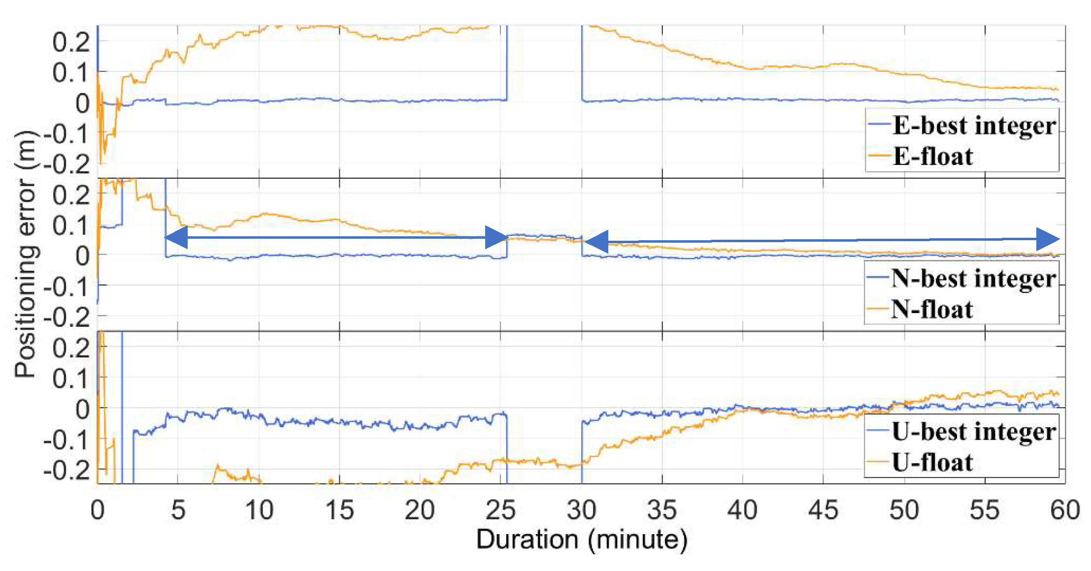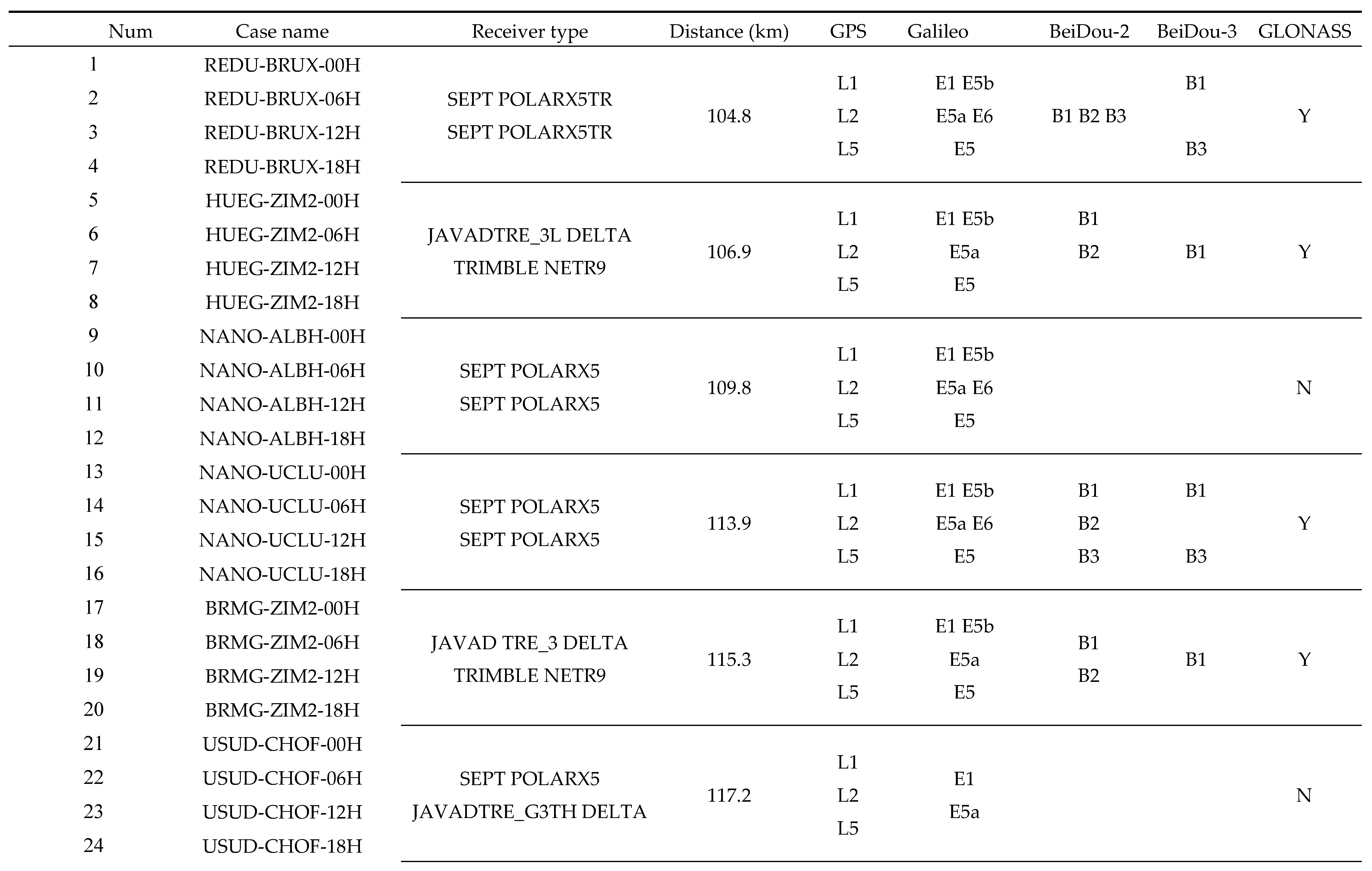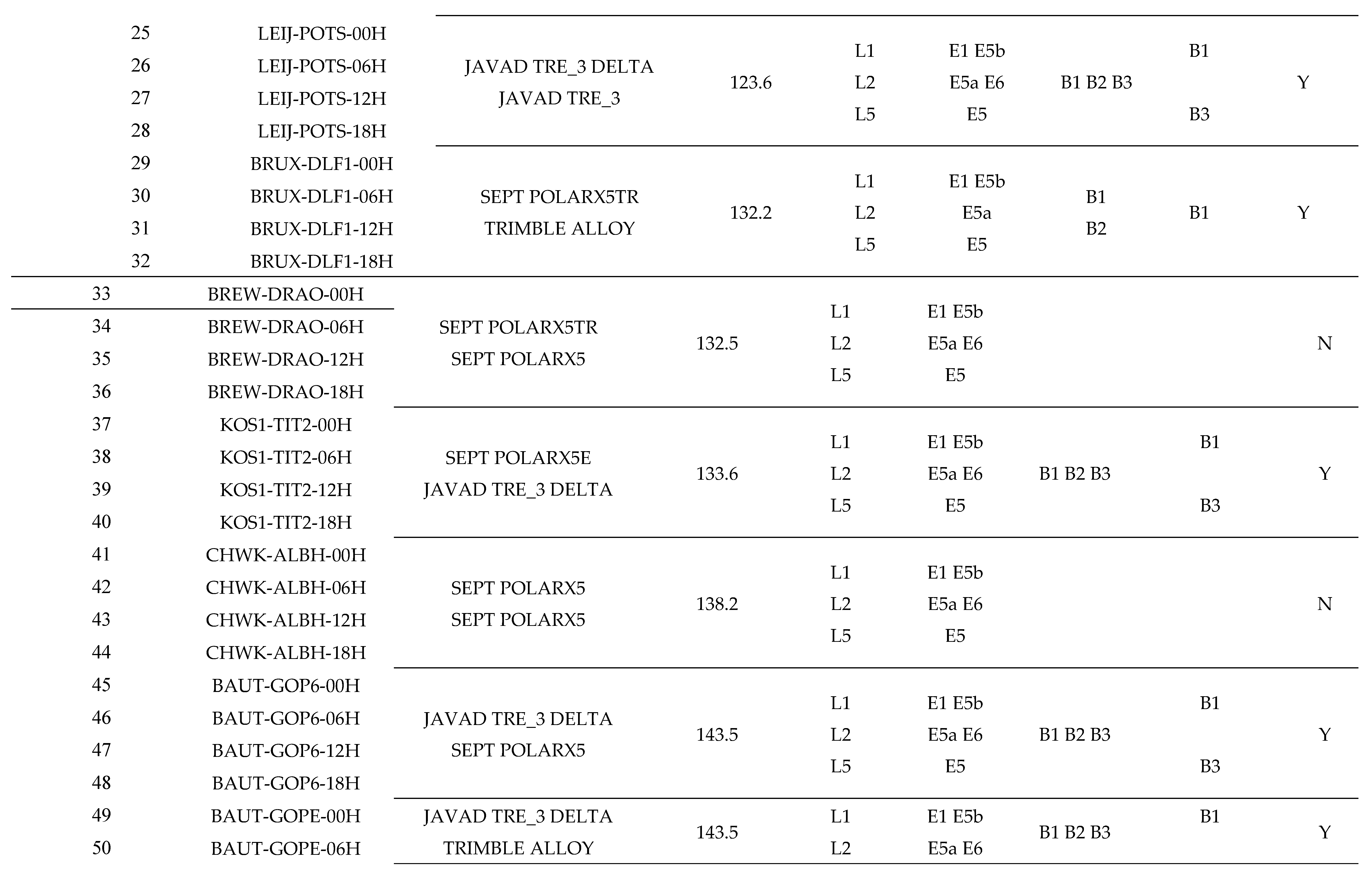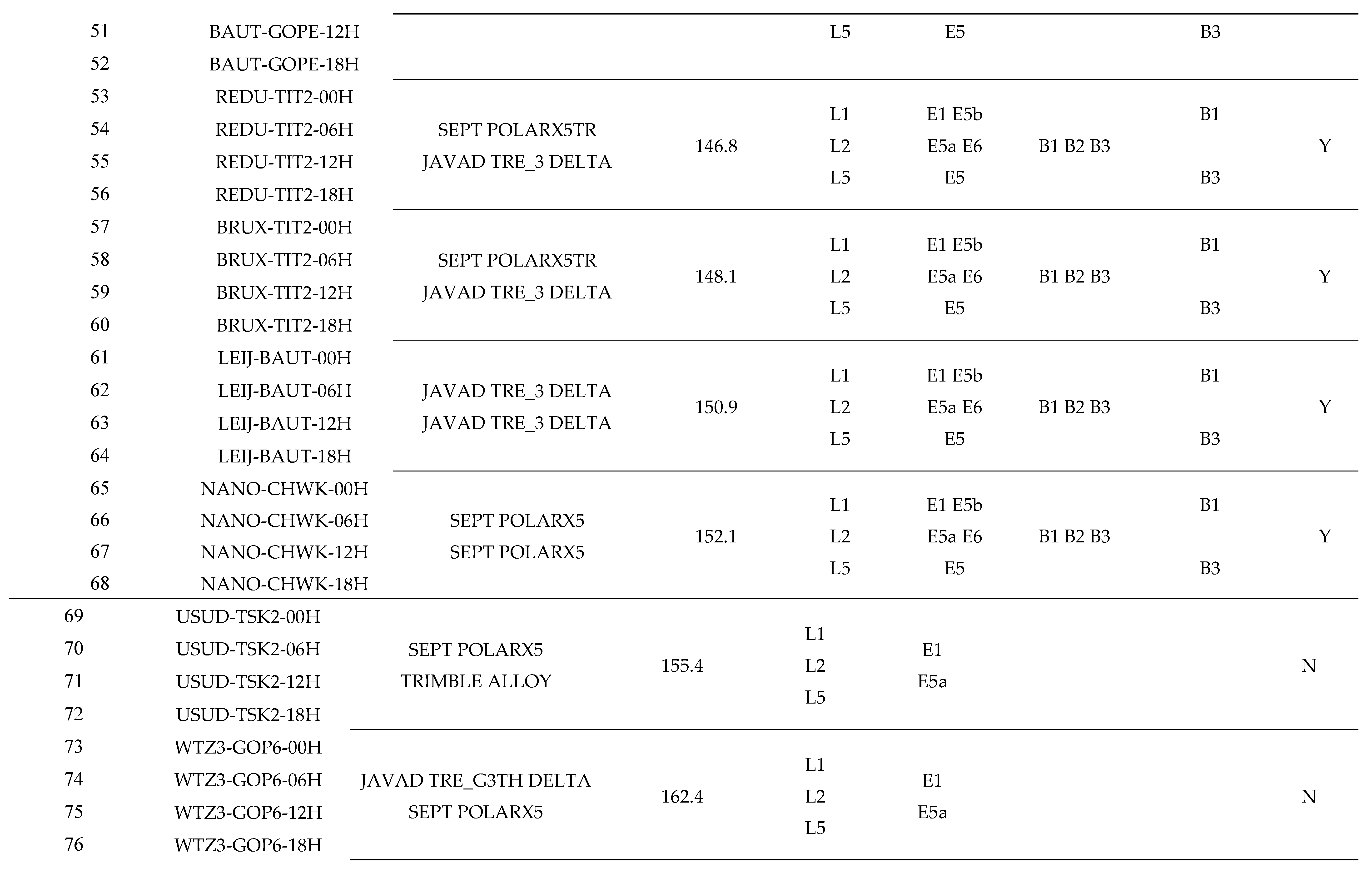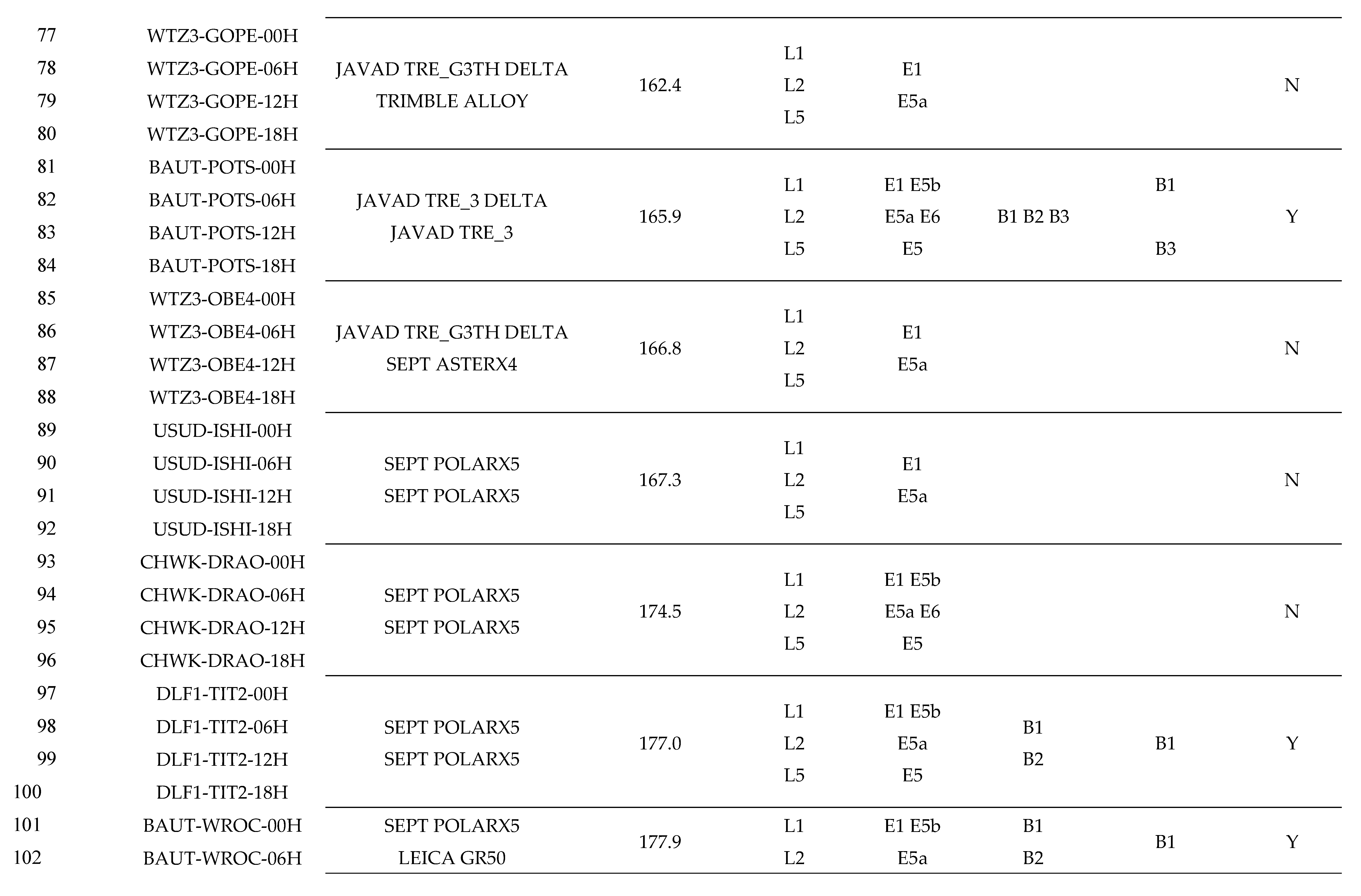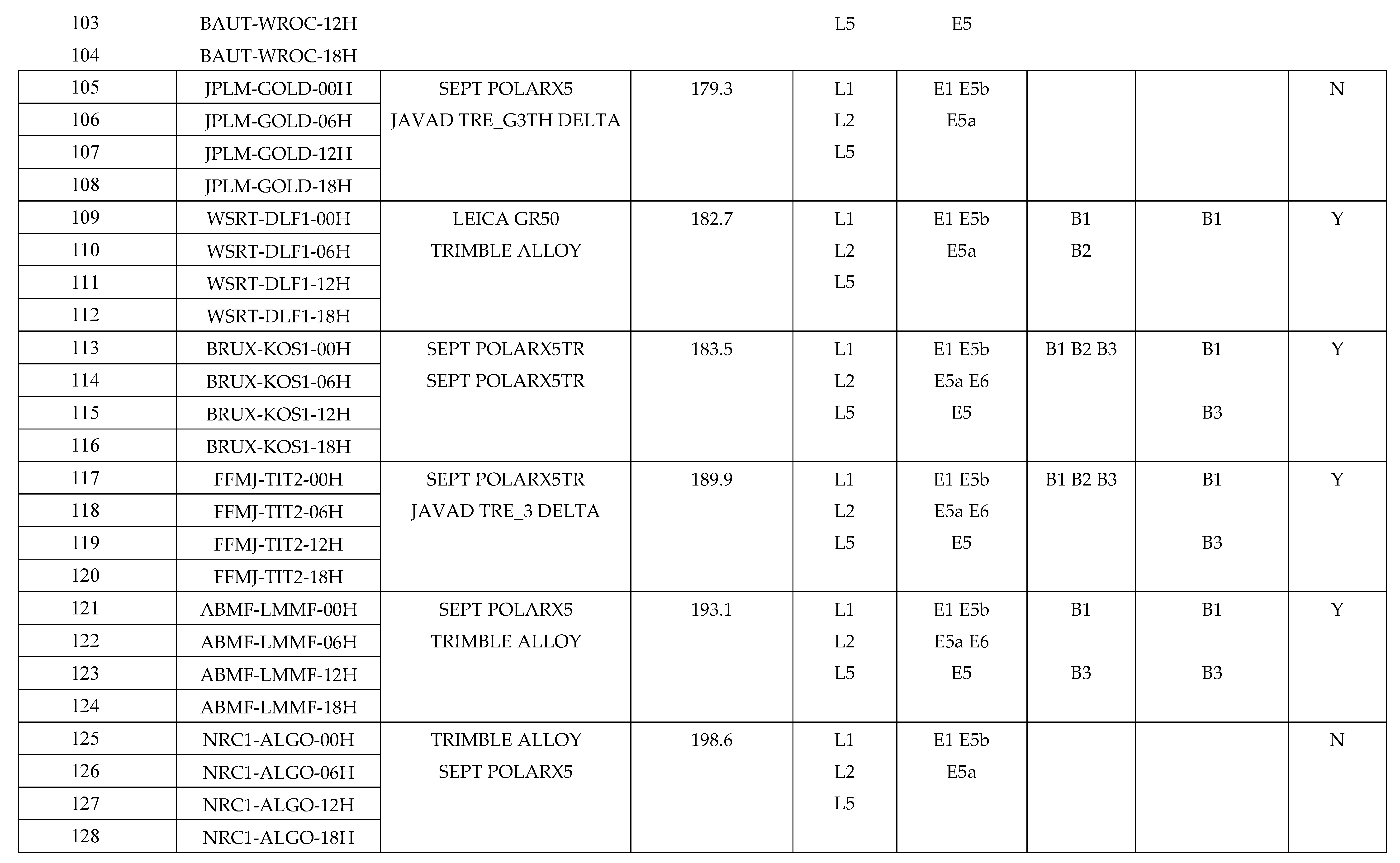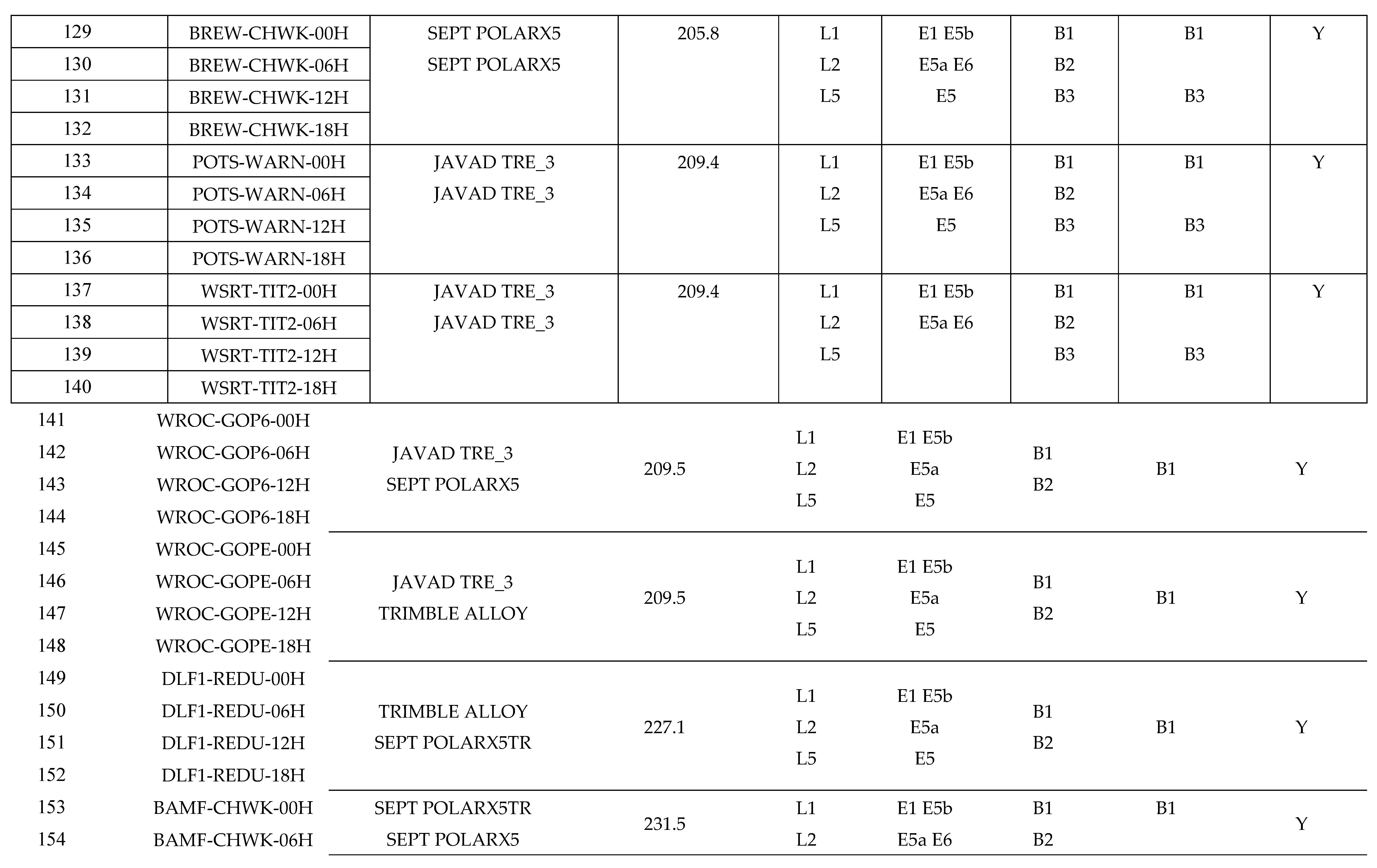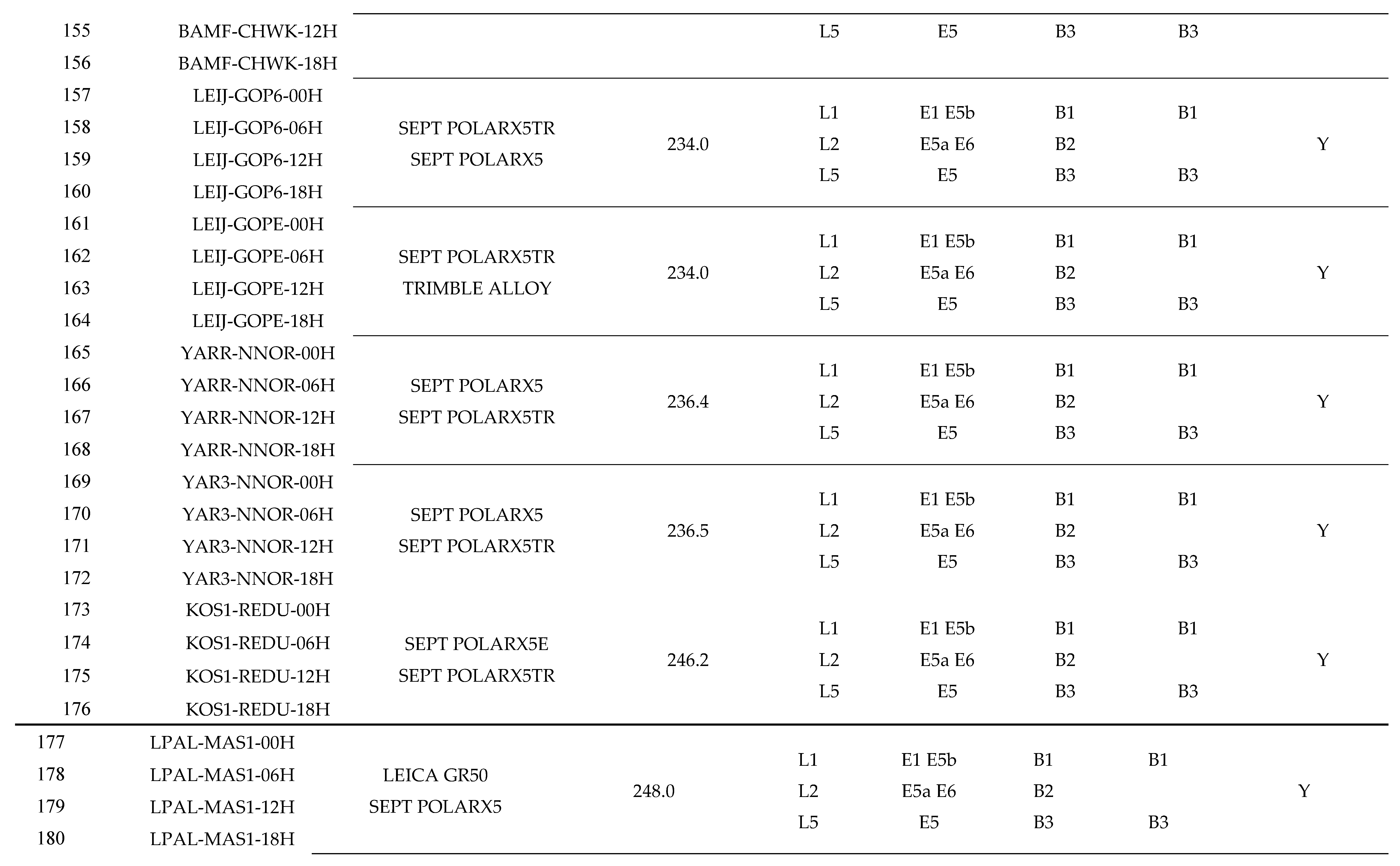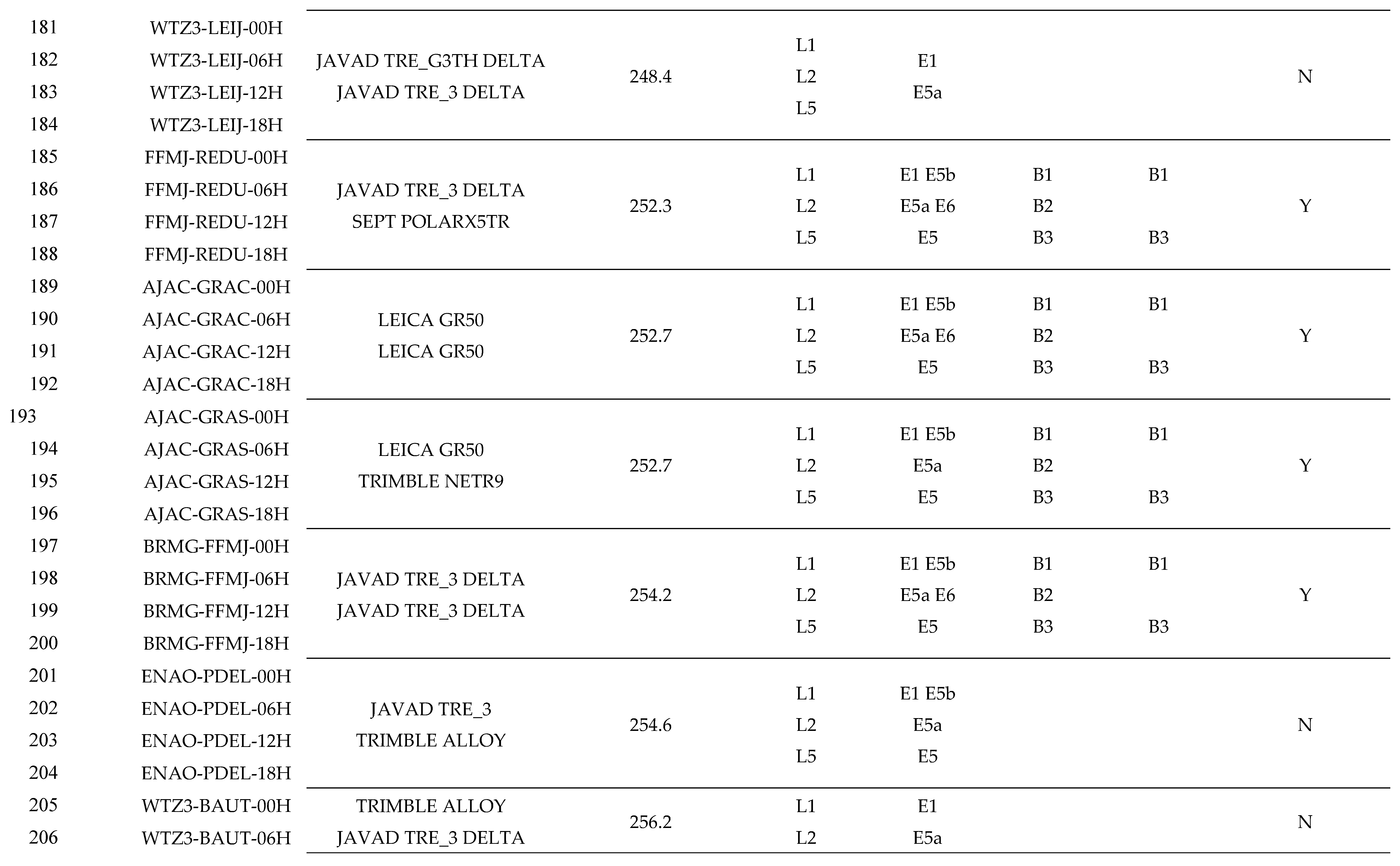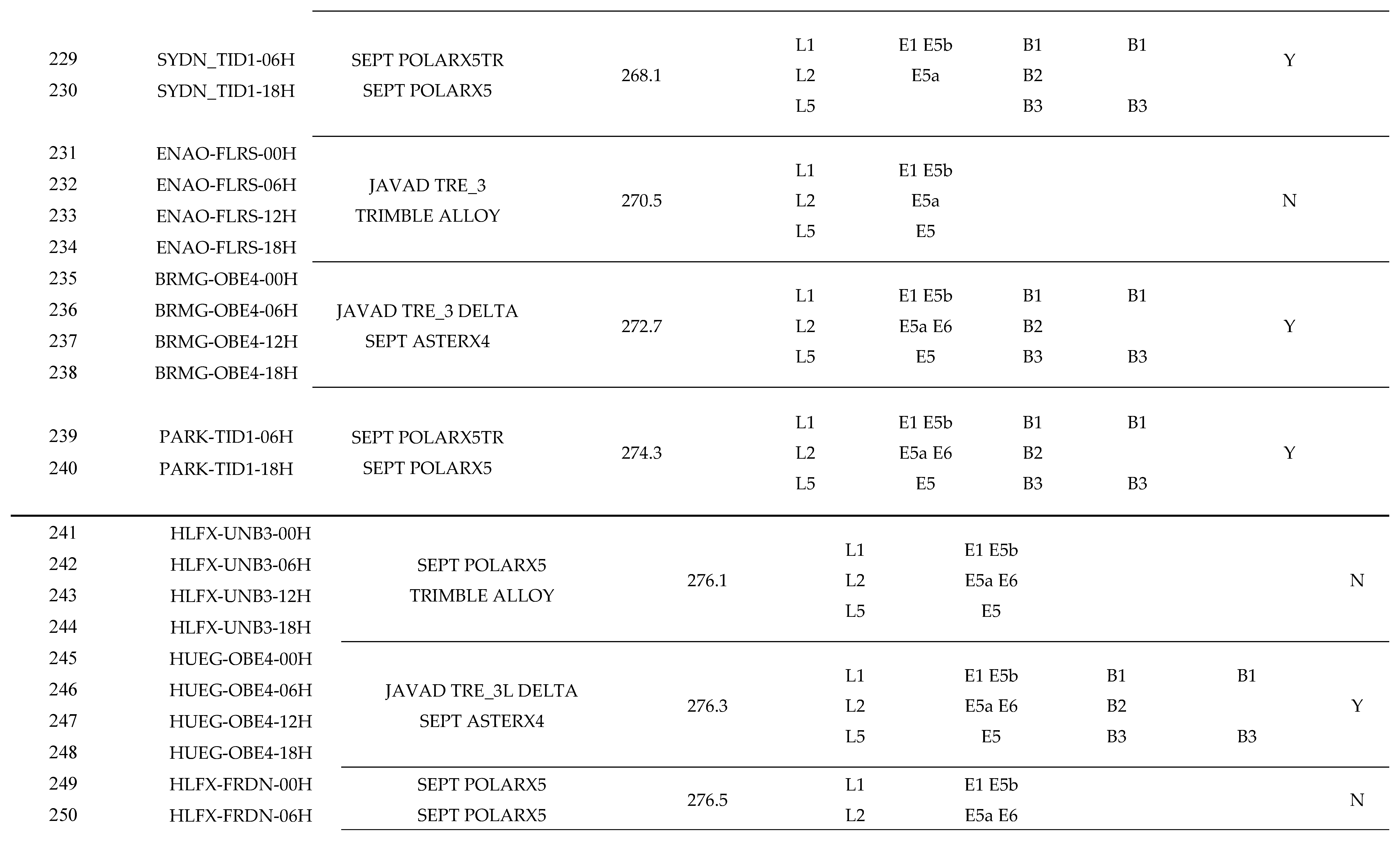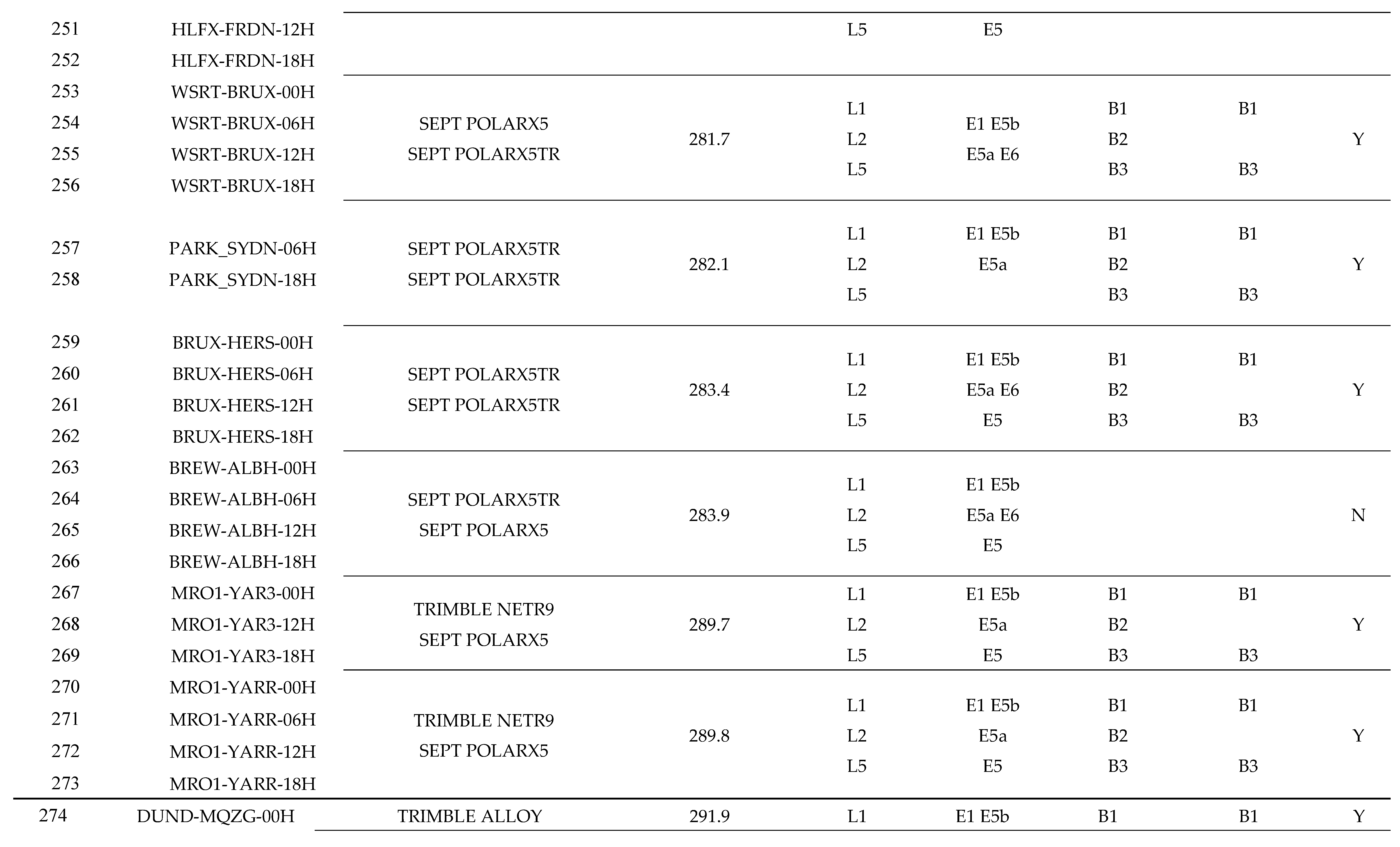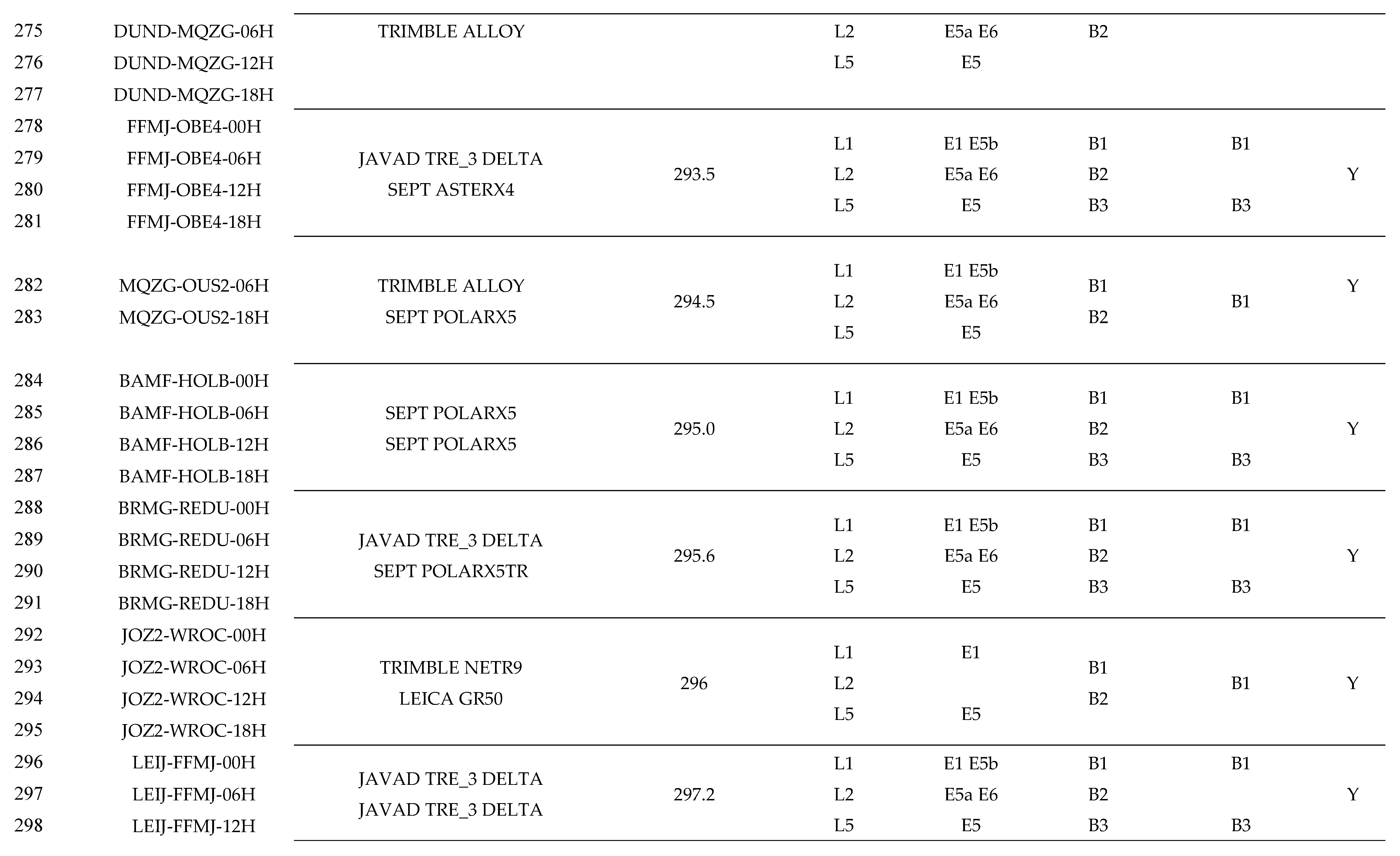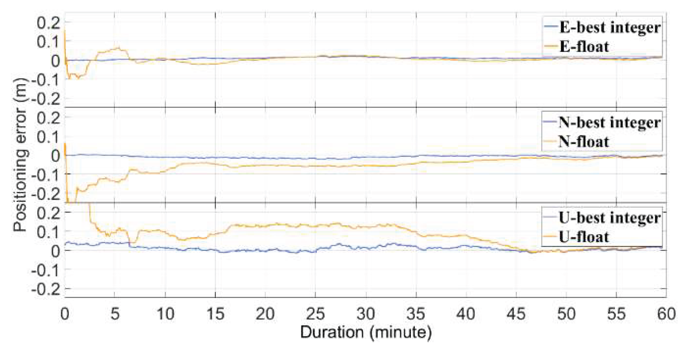Figure 2 illustrates the positioning errors for the best ambiguity resolution (in blue) and the float solution (in red) for experimental case No. 125. The two periods marked by arrows represent the intervals of one ambiguity resolution, and their combined length constitutes the total duration of this resolution. Cases that fail to meet these criteria are excluded from the study. After applying these filters, 307 experimental cases remained and were sequentially numbered. 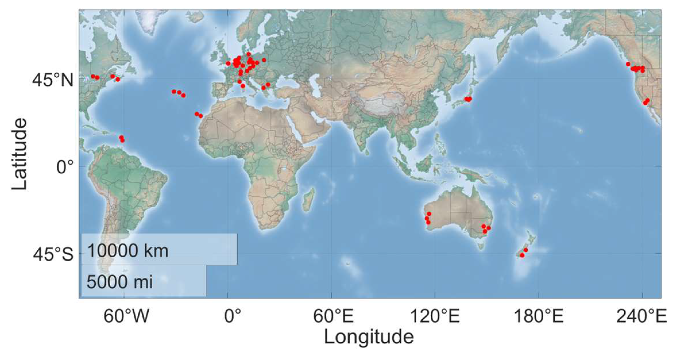Detailed information on the experimental cases can be found in Appendix A. The global distribution of the cases is shown in Figure 2.

Figure 1. Positioning errors of experimental case No. 125.

Figure 2. Global distribution of the experimental baselines.

4. Numerical Results

In this section, we present a detailed examination of the experimental outcomes. Initially, we provide a synopsis of the performance in resolving ambiguities, followed by an assessment of the performance in validating ambiguities, which includes an analysis of the theoretical success rate and the R-ratio test.

4.1. Overview of the Experimental Results

The objective of this subsection is to give an overview of ambiguity resolution performance, including the minimum time required to fix ambiguity, the R-ratio performance in one minute and one hour, and a comparison of convergence time and positioning accuracy between the best and float ambiguity resolution.

4.1.1. Minimum Required Time to Fix Ambiguity

Here, we explore the earliest time of the best integer ambiguity resolutions being able to be determined to be correct and subsequently remains constant as shown in Figure 3 or stable in spite of interruption as shown in Figure 1. Theoretically, it should represent the minimum time necessary to resolve ambiguities, irrespective of the ambiguity validation method employed.

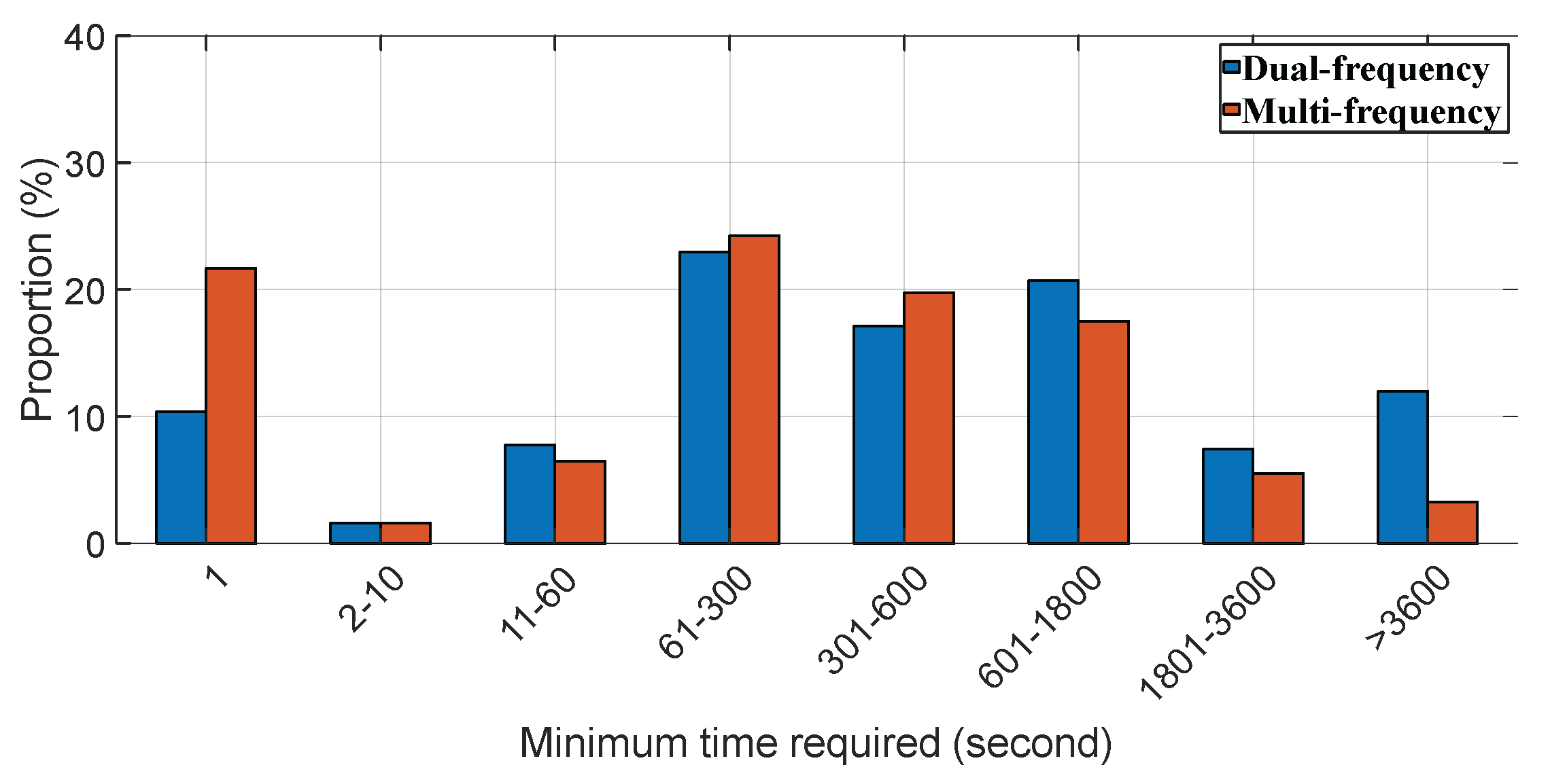
Figure 4 displays the minimum time necessary to correctly resolve ambiguities, with the left side pertaining to dual-frequency scenarios and the right side to multi-frequency scenarios. Figure 5 provides statistical analysis of these times. It is evident that in both scenarios, there are instances where ambiguities can be correctly fixed in a single epoch; approximately 10% of such cases occur in dual-frequency scenarios, while the figure exceeds 20% for multi-frequency scenarios. For the remaining experimental cases, the minimum time required to resolve ambiguities typically ranges from one minute to thirty minutes. Additionally, in both scenarios, there are instances where ambiguities cannot be resolved correctly even after one hour.

4.1.2. Maximum R-Ratio in One Minute and One Hour

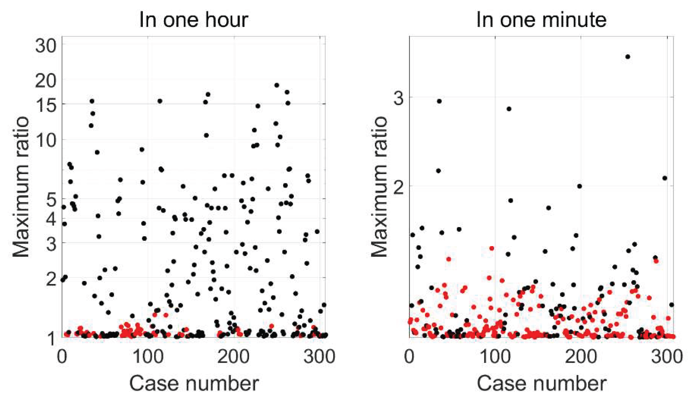
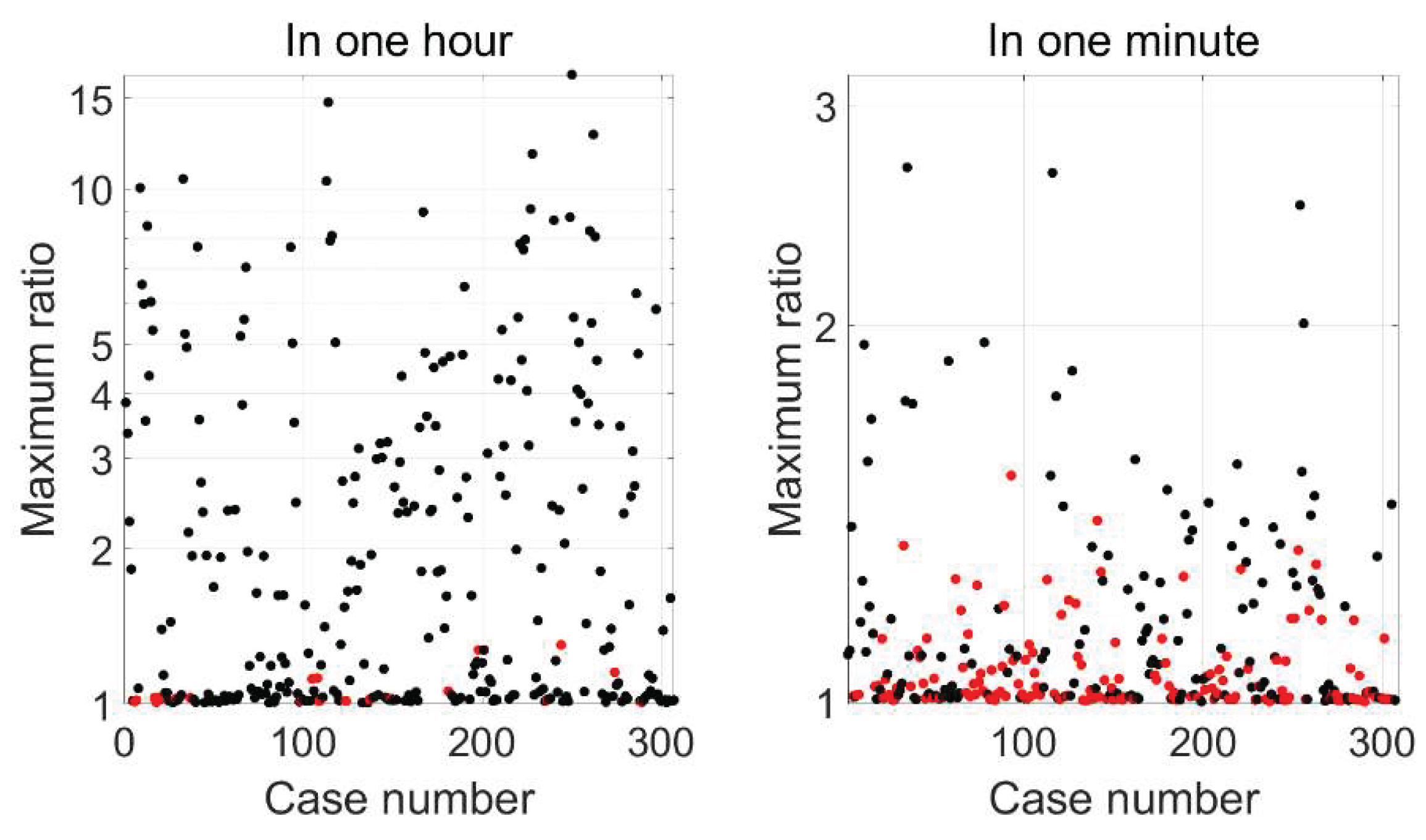
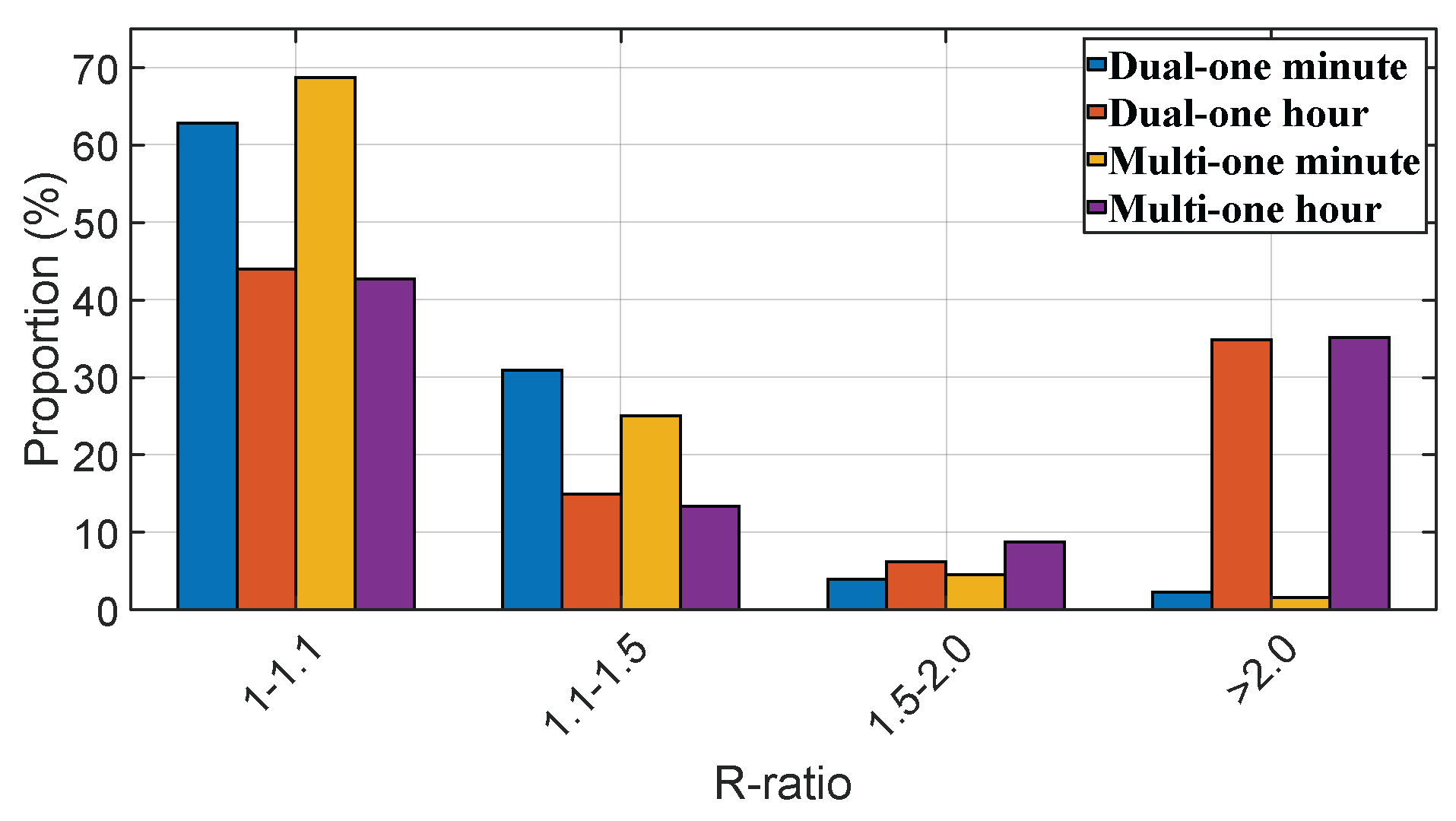
Figure 6 and Figure 7 present the maximum R-ratio values attained within one minute and one hour, respectively, for both dual- and multi-frequency scenarios. Black dots represent instances of correct ambiguity resolution, whereas red dots denote incorrect resolutions. Figure 8 compiles statistics of the peak R-ratio values observed.

From the data, it is apparent that in both dual- and multi-frequency scenarios, the majority of the maximum R-ratio values cluster between 1.0 and 1.1, regardless of whether the duration is one minute or one hour. Approximately 35% of the experimental cases exhibit an R-ratio greater than 2.0 after an hour, in contrast to only about 2% reaching the level within one minute.

4.1.3. Convergence Time

Convergence time to reach centimeter-level accuracy is usually used as a measure to assess the performance with float ambiguity resolution in both PPP and long-distance RTK. In this section, the convergence time is also investigated with the best integer ambiguity resolution no matter it is correct or not and compared to that of the float ambiguity resolution.

Figure 9 depicts the time required for positioning errors in both the north and east directions to fall below 10 cm. The blue bar represents the best integer ambiguity resolution. It is observed that, in the dual-frequency scenario illustrated on the left, over 10% of the experimental cases achieve centimeter-level accuracy in a single epoch, whereas in the multi-frequency scenario on the right, this figure rises to about 25%. However, for the remaining cases, reaching such accuracy typically requires between one minute and thirty minutes. The red bar indicates the float ambiguity resolution. In both dual- and multi-frequency scenarios, less than 1% of cases achieve the desired accuracy in a single epoch, with the necessary time predominantly ranging from 10 minutes to thirty minutes.

Figure 10 shows the convergence time in the vertical direction, with results mirroring those in the horizontal directions. Thus, in terms of convergence time, the best integer ambiguity resolution, regardless of its correctness, outperforms the float solution. However, in practical settings, the float ambiguity resolution is more commonly used than the best integer solution, likely due to the higher risk of significant positioning errors associated with the latter.

4.1.3. Positioning Accuracy

This section aims to compare the positioning accuracy with correct integer ambiguity resolution if it can be fixed successfully to that with converged float ambiguity solution in the latter half hour of the hourly session.

Figure 11, Figure 12 and Figure 13 depict the positioning RMS in east, north and vertical directions. The benefit of correct ambiguity resolution is substantial with almost all positioning RMS much less than 5 cm in all directions. While for float ambiguity resolution, most RMS are around 5 cm and there are cases with RMS reaching several decimeters.

4.2. Ambiguity Validation with the Theoretical Success Rate of Ambiguity Resolution

The theoretical success rate of ambiguity resolution is often used for ambiguity validation, particularly for short-distance baseline. This study extends the investigation of its effectiveness to long-baseline scenarios. Initially, we introduce the upper and lower bounds, as well as an approximation of the success rate, following by the presentation of experimental findings.

The success rate of ambiguity resolution can be calculated according to the following formula:

P_{s} = P (\overset{ˇ}{N} = N) = \int_{P_{N}}^{​} f_{\hat{N}} (x | N) d x

(3)

where,

P_{N}

is the pull-in region,

N = {N_{1}, N_{2}, \dots, N_{n}} i s c o r r e c t a m b i g u i t y,

\hat{N}

and

\overset{ˇ}{N}

are float and integer ambiguity resolution respectively.

f_{\hat{N}} (x | N)

is assumed to be the normal PDF of

\hat{N}

with mean

N

and VC-matrix

Q_{\hat{N} \hat{N}}

Calculating the exact success rate

P_{s}

, is highly complex due to the intricate nature of

P_{N}

. Consequently, in practical scenarios, approximations or bounds are utilized instead.

The first upper bound by bounding the pull-in region is given as (Teunissen 1998a):

P_{U p p e r, 1} = \prod_{i = 1}^{p} (2 Φ (\frac{1}{2 σ_{v_{i | I}}}) - 1)

(4)

With

p < n

and

σ_{v_{i} v_{j}} = \frac{u_{i}^{T} Q_{\hat{N} \hat{N}} u_{j}}{‖u_{i}‖ Q_{\hat{N} \hat{N}} ‖u_{j}‖ Q_{\hat{N} \hat{N}}}

u_{i}

和

u_{j} \in Z^{n}

The second upper bound for Integer Least Squares (ILS) based on ADOP is given as (Hassibe and Boyd 1998; Teunissen 2000):

P_{U p p e r, 2} = P (χ^{2} (n, 0) \leq \frac{C_{n}}{{A D O P}^{2}})

(5)

With

C_{n} = \frac{{(\frac{2}{n} Γ (\frac{2}{n}))}^{\frac{2}{n}}}{π}

and

A D O P = {\sqrt{d e t (Q_{\hat{N} \hat{N}})}}^{\frac{1}{n}}

An approximation to the ILS success rate based on ADOP can be calculated as (Teunissen 2000):

P_{A p p r o x i m a t i o n} = {(2 Φ (\frac{1}{2 A D O P}) - 1)}^{n}

(6)

The first lower bound with bootstrapping (IB) can be calculated as (Teunissen 1998b):

P_{L o w e r, 1} = \prod_{i = 1}^{n} (2 Φ (\frac{1}{2 σ_{{\hat{N}}_{i | I}}}) - 1)

(7)

where

σ_{{\hat{N}}_{i | I}}

with

I = {i + 1, \dots, n}

is the conditional variance of the

i

th float ambiguity

{\hat{N}}_{i}

on the float ambiguities from

i + 1

n

The second lower bound with Integer Rounding (IR) based on the diagonal VC-matrix

Q_{\hat{N} \hat{N}}

can be calculated as (Teunissen 1998b):

P_{L o w e r, 2} = \prod_{i = 1}^{n} (2 Φ (\frac{1}{2 σ_{{\hat{N}}_{i}}}) - 1)

(8)

where

σ_{{\hat{N}}_{i}}^{2}

is the diagonal element of

Q_{\hat{N} \hat{N}}

The third lower bound by bounding the pull-in region is given as:

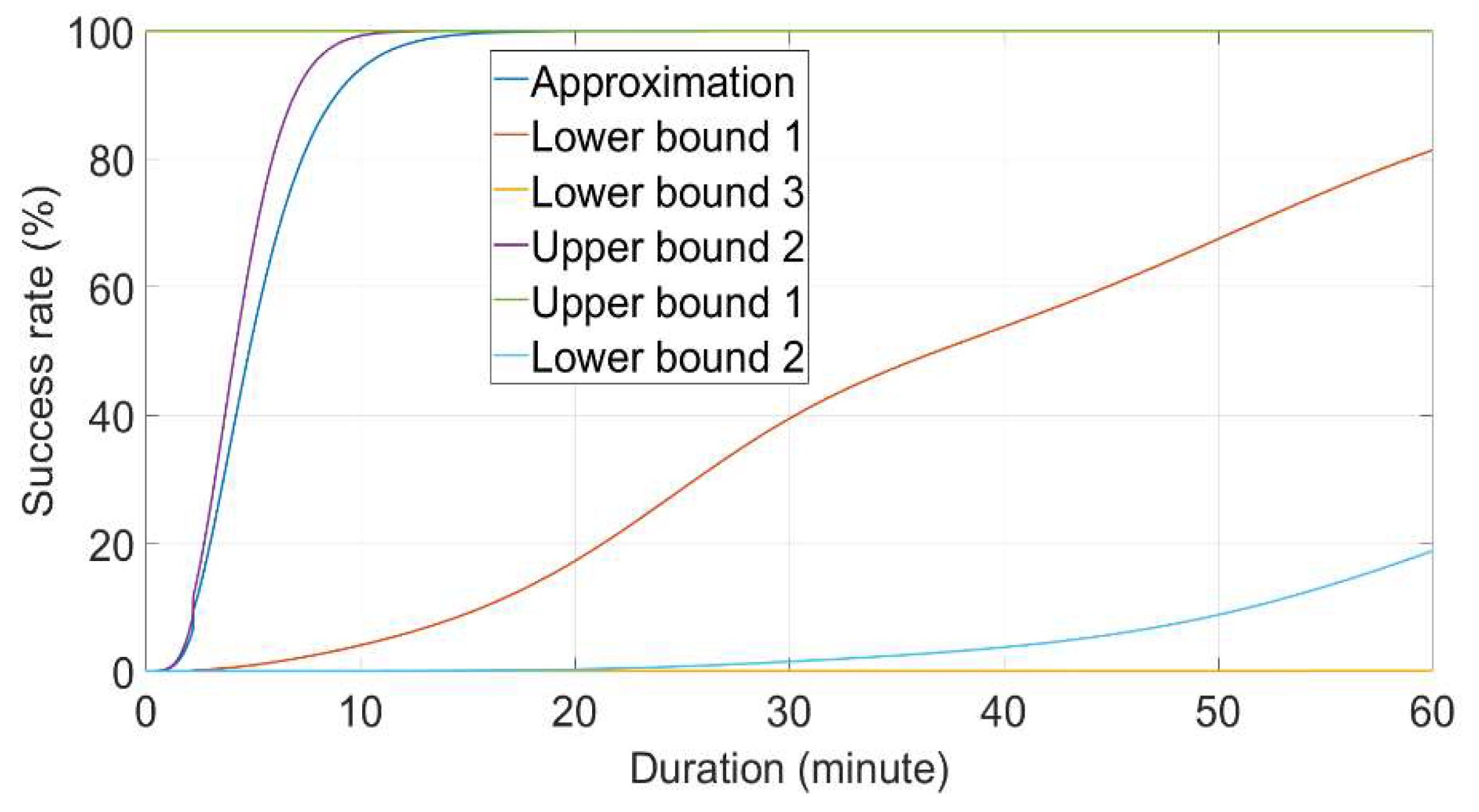
P_{L o w e r, 3} = P (χ^{2} (n, 0) \leq \frac{1}{4} \min_{u \in Z^{n} \ \{0\}} {‖u‖}_{Q_{\hat{N} \hat{N}}}^{2})

(9)

Figure 14 illustrates six different success rates over varying time durations for the experimental case involving shows these six success rates with different durations for the experimental case No. 88 (dual-frequency). The graph reveals a substantial disparity between the highest,

P_{U p p e r, 1}

and the lowest,

P_{L o w e r, 3}

, with a potential difference nearing 100%.

P_{U p p e r, 1}

approaches 100% within a single epoch, while

P_{U p p e r, 2}

and

P_{A p p r o x i m a t i o n}

exhibit similar treads, both achieving approximately 99.9% within a 10 to 20-minute span.

P_{L o w e r, 1}

surpasses the 80% threshold after one hour, whereas

P_{L o w e r, 2}

does not exceed 20% even after the same duration.

P_{L o w e r, 3}

remains negligible, barely deviating from zero after one hour.

And the order of the six success rates is:

P_{U p p e r, 1} > P_{U p p e r, 2} > P_{A p p r o x i m a t i o n} > P_{L o w e r, 1} > P_{L o w e r, 2} > P_{L o w e r, 3}

The observed consistency in the order of these six success rates across all the experimental cases suggests that the exact success rate is likely to fall between

P_{U p p e r, 2}

and

P_{L o w e r, 1}

or between

P_{A p p r o x i m a t i o n}

and

P_{L o w e r, 1}

. This observation implies that

P_{U p p e r, 1}

P_{L o w e r, 2}

and

P_{L o w e r, 3}

may not be suitable for practical applications.

To establish the range of the exact success rate more precisely, Figure 15 displays the minimum time required for

P_{A p p r o x i m a t i o n}

to achieve a 99.999% success rate across all experimental cases, considering both dual- and multiple-frequency scenarios. Black dots indicate cases where the best integer ambiguity resolution is correct, while red dots represent incorrect resolutions. For dual-frequency cases, 50% requires less than 5 minutes to reach this level of success, and 74.3% require less than 10 minutes. In contrast, for multiple-frequency cases, 50% achieve this success rate in under half a minute, and 69.4% in under one minute. However, the prevalence of red dots indicates that the majority of cases are incorrect, 62.5% for dual-frequency and 64.2% for multiple-frequency. This suggests that

P_{A p p r o x i m a t i o n}

is likely significantly higher than the exact success rate, rendering it inapplicable as well.

to reach 99.999% (left: dual frequency; right: multi-frequency).

Consequently, it is reasonable to infer that the exact success rate should be bracketed between

P_{A p p r o x i m a t i o n}

and

P_{L o w e r, 1}

Figure 16 presents

P_{L o w e r, 1}

success rates for dual- and multiple-frequency cases after a one-hour duration. Black dots denote cases with correct best integer ambiguity resolution, and red dots denote incorrect resolutions. Additionally, Figure 17 provides statistics on the distribution of different

P_{L o w e r, 1}

values. For dual-frequency cases, 45.28% have

P_{L o w e r, 1}

greater than 90%, and 71.34% have

P_{L o w e r, 1}

greater than 80%. For multi-frequency cases, these figures are 77.20% and 89.25%, respectively. Notably, in both dual- and multi-frequency scenarios, only one case resulted in incorrect best integer ambiguity.

Therefore, among the six evaluated success rates,

P_{L o w e r, 1}

appears to be the closest approximation to the exact success rate. Furthermore, Figure 17 indicates that, regardless of whether the frequency is dual or multiple, most cases can be correctly resolved within a one-hour duration.

In summary, the investigation reveals that the two upper bounds and the approximation, along with

P_{L o w e r, 2}

and

P_{L o w e r, 3}

, deviate significantly from the exact success rate, being either excessively high or markedly low. Consequently, these metrics are not suitable for practical application in long-distance RTK. Although

P_{L o w e r, 1}

appears to be the closest to the exact success rate, its utility is limited to scenarios where long observation durations are feasible. Therefore, for practical long-distance RTK applications, reliance on

P_{L o w e r, 1}

may only be advisable when extended observation times are available to ensure a higher likelihood of correct ambiguity resolution.

4.3. Ambiguity Validation with R-Ratio Test

The R-ratio test is widely used in network RTK for its high reliability, typically with a threshold value of 2.0. This section delves into the R-ratio test’s performance and efficacy for long-distance RTK applications.

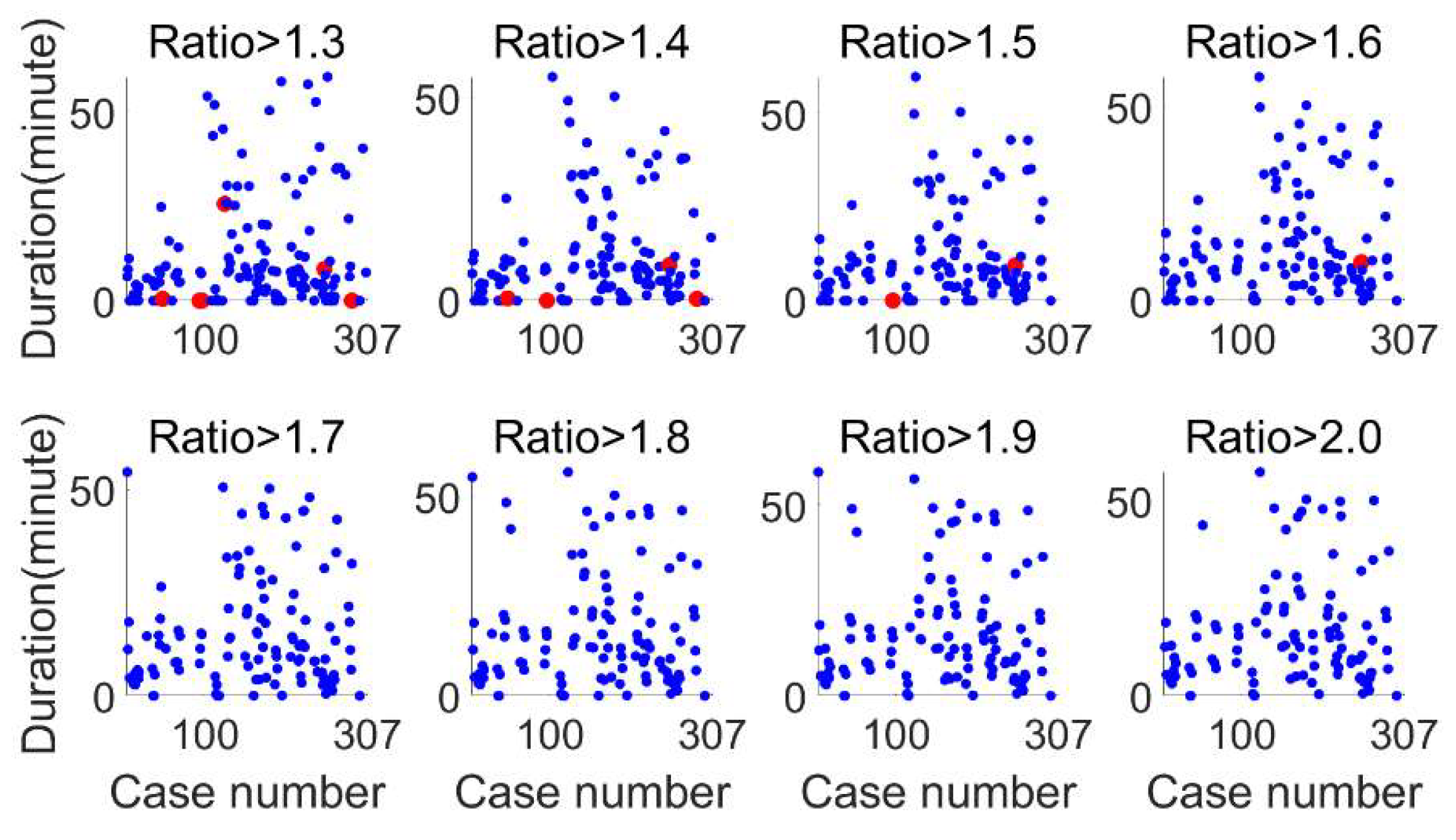
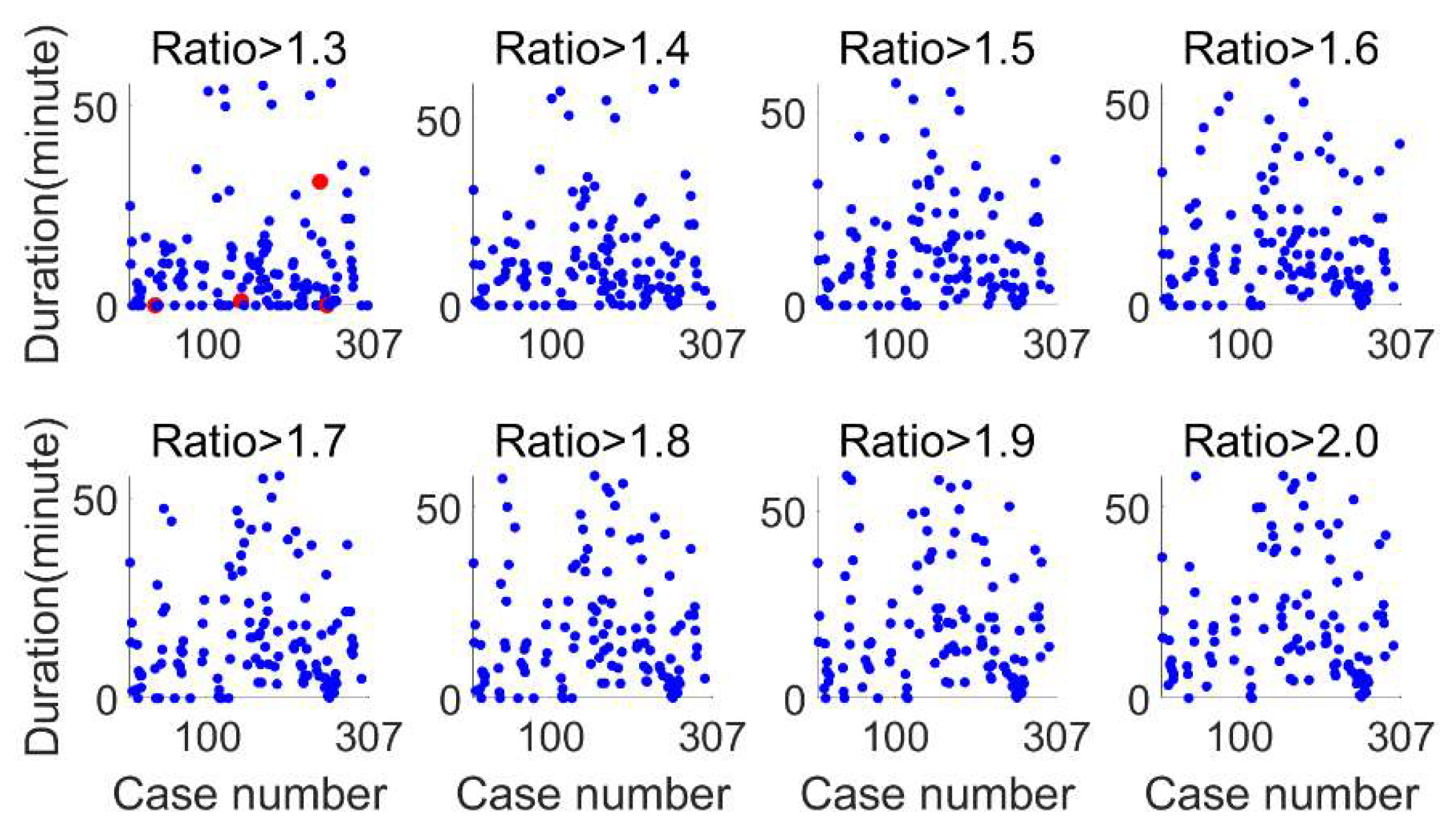
Figure 18 and Figure 19 display the minimum time required for the R-ratio to exceed various thresholds, 1.3, 1.4, 1.5, 1.6, 1.7, 1.8, 1.9 and 2.0, for both dual- and multi-frequency scenarios. Black dots indicate correct ambiguity resolution, while red ones signify mis-fix.

In the dual-frequency scenario, mis-fixes occur at the threshold values of 1.3, 1.4, 1.5 and 1.6, with mis-fix count of 6, 4, 2 and 1, respectively. For multi-frequency, mis-fixes are observed only at a threshold value of 1.3, totaling four cases. The specifics of these mis-fixes are detailed in Table 2. It is observed that for dual-frequency, mis-fixed can be attributed to either a short duration, no longer than 1 minute, or a limited number of satellites, no more than 8. Similarly, for multi-frequency, one mis-fix occurred with a duration exceeding half an hour but with only 5 satellites observed, while the durations for the other three mis-fixes were 4, 4, and 69 seconds, respectively, barely over a minute.

Table 2 presents the counts and percentages of successful ambiguity resolutions across different threshold values for dual- and multi-frequency scenarios. It is noted that, regardless of frequency, the success rate does not exceed 50% even at a threshold of 1.3, and it marginally surpasses one-third when the threshold is set to 2.0. Furthermore, the success rates for dual- and multi-frequency are quite comparable. For dual-frequency, the success rates range from 44.6% to 34.9% and for multi-frequency, from 46.3% to 35.2%.

Table 3. Statistics of success ambiguity resolution of various R-ratio threshold.

threshold	dual-frequency		multi-frequency
threshold	case count	proportion (%)	case count	proportion (%)
1.3	137	44.6	142	46.3
1.4	128	41.7	141	45.9
1.5	124	40.4	135	44.0
1.6	122	39.7	132	43.0
1.7	117	38.1	123	40.1
1.8	114	37.1	123	40.1
1.9	111	36.2	115	37.5
2.0	107	34.9	108	35.2

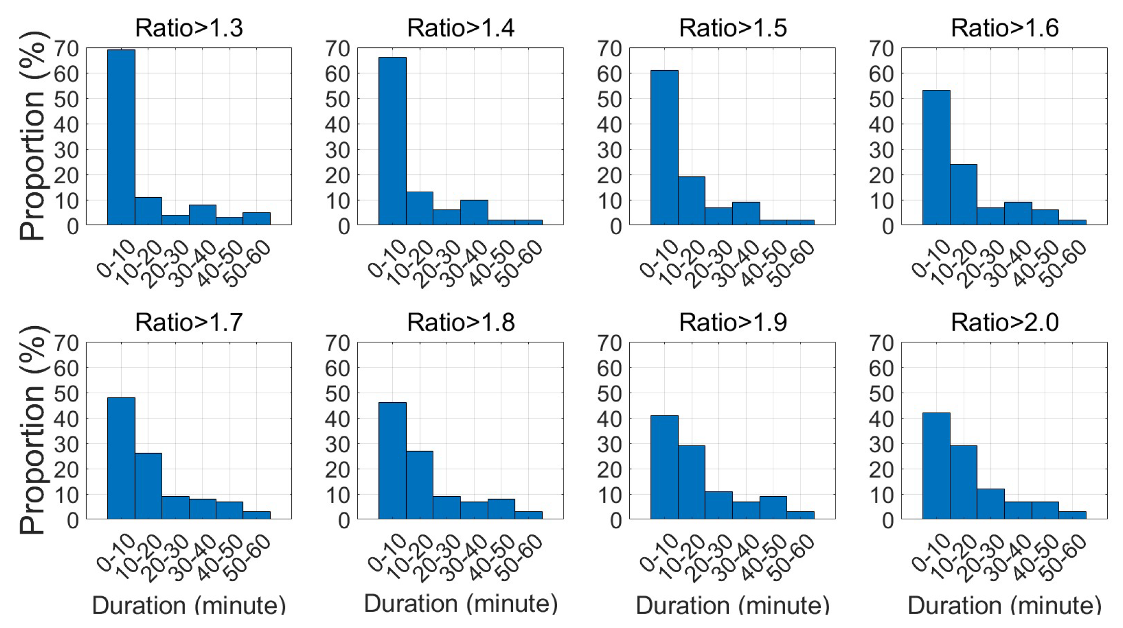
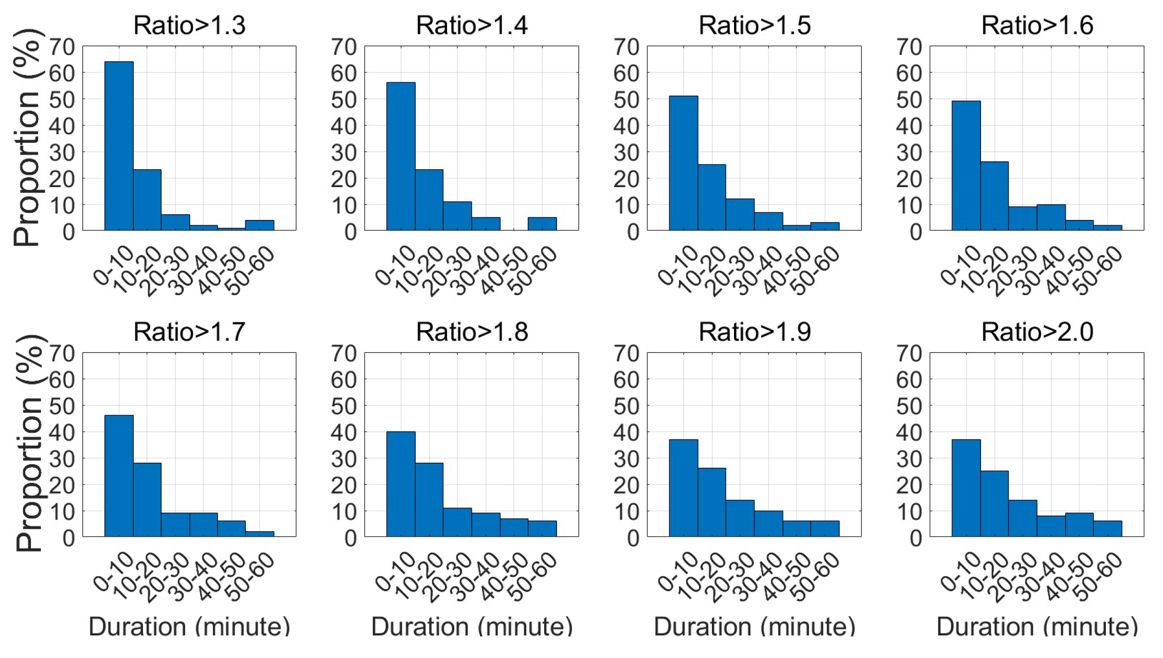
Figure 20 and Figure 21 provide statistical data on the time needed to achieve various R-ratio thresholds for both dual- and multi-frequency scenarios. Across all threshold values, for both dual- and multi-frequency, the most common duration to reach the threshold is within 10 minutes, followed by the 10 to 20-minute range as the second most common. When the threshold is set to 2.0, approximately 70% of dual-frequency cases and 60% of multi-frequency cases reach the threshold within 20 minutes. This suggests that if the R-ratio does not meet the threshold within 20 minutes, it is unlikely to succeed in fixing the ambiguity even with extended observation time.

To conclude, the R-ratio test tends to be more dependable for ambiguity validation when the observation duration exceeds 2 minutes and when there are more than 10 satellites being observed. A threshold value above 1.7 is recommended for better reliability. If the threshold is attainable, the required observation duration is typically no more than 20 minutes; otherwise, merely prolonging the observation time is unlikely to help the ratio meet the threshold. Additionally, the overall success rate for ambiguity resolution using the R-ratio test is relatively low, not exceeding 50% even at a threshold of 1.3, and hovering around one-third when the threshold is set to 2.0.

5. New Ambiguity Resolution Validation Method

Based on the findings, it is evident that the six theoretical success rate bounds do not align well with practical outcomes for long-distance RTK, as there is a significant discrepancy between their values and the actual ones. In the case of the R-ratio test, although it appears to be a reliable indicator with a threshold value exceeding 1.7, the likelihood of successful ambiguity resolution remains disappointingly low, dropping to merely one-third when the threshold is set at 2.0. Consequently, it appears that, for the cases unable to be fixed with the R-ratio test, resorting to float ambiguity resolution is the only viable option, which however is sometimes unreasonable.

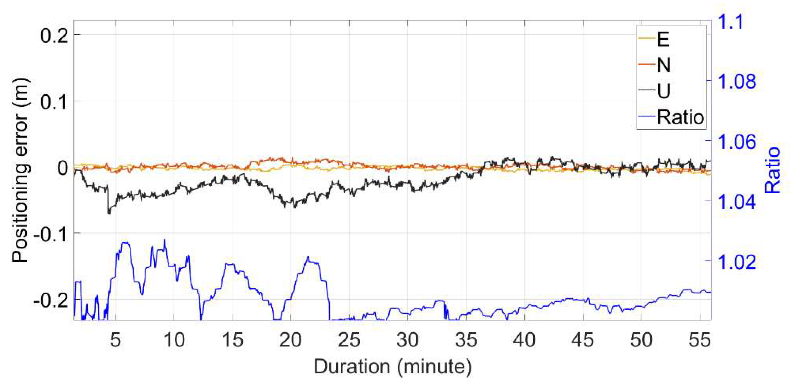
Illustrating this point, Figure 22 shows the experimental case No. 31 (multiple-frequency) and presents the positioning errors in the X, Y, and Z directions using both the best integer and float ambiguity resolutions, alongside the R-ratio values. The data reveals that the best ambiguity resolution is correct from onset. However, throughout the hour, the R-ratio value does not exceed 1.05. Employing the float solution may result in significantly reduced positioning accuracy compared to the integer solution, even after thirty minutes, which is both illogical and inefficient.

In this section, we introduce a novel method for validating ambiguity resolution that is tailored for scenarios where the R-ratio test may not be effective. Unlike conventional approaches that prioritize rapid ambiguity resolution within a few minutes or up to twenty minutes, our proposed method is designed to be applicable over more extended periods, such as thirty minutes to an hour.

Figure 23 depicts the duration for which a particular ambiguity candidate remains the best integer ambiguity resolution (indicated in blue) in comparison to the second-best candidate (shown in greed) over the course of an hour. These durations can be either continuous or intermittent. In instances where the ambiguity resolution with the longest duration is incorrect, it is marked in red. Additionally, a yellow line represents the ratio of the second-longest duration to the longest duration.

Analysis of the left part reveals that for dual-frequency data, the majority of the best ambiguity resolutions with the longest durations are accurate. However, there is an 8.79% incidence of incorrect resolutions. Within this subset, there are 27 instances that exceed 10 minutes, yet all fall short of the half-hour mark, with one exception lasting 2036 seconds.

Turning to the right part, which focuses on multi-frequency data, we observe that incorrect cases are present, albeit at a lower rate of 0.65%, Among these, only two cases surpass the 10-minute threshold, and none extend beyond 1000 seconds. This suggests that the proposed method may offer a more reliable means of ambiguity validation over longer periods, particularly in multi-frequency scenarios where the duration of incorrect resolutions is notably shorter.

6. Conclusions

In this study, which utilizes extensive data from the IGS network, a comprehensive analysis was conducted on the effectiveness of two widely adopted ambiguity validation techniques in long-distance RTK. The fundings from the numerical analysis indicate that:

➢: The six theoretical success rate bounds currently in use are either excessively large or small compared to the actual value, rendering them impractical for long-distance RTK applications.
➢: The R-ratio test proves to be generally reliable when the threshold is set above 1.7, provided that there is an adequate duration of observations (at least one minute) and a sufficient number of visible satellites (more than 10).
➢: The likelihood of successfully resolving ambiguities using the R-ratio test does not exceed 50%. Furthermore, if a resolution is not achieved in 20 minutes, merely extending the observation time is typically ineffective.
➢: In spite of different time required to exceed various R-ratio thresholds, the success rates for dual- and multi-frequency are quite comparable.

To enhance ambiguity resolution performance in practical scenarios that involve lengthy observation periods, this research introduces a new ambiguity validation approach. This method suggests that if one integer ambiguity resolution candidate maintains the best status for a significantly longer period than its runner-up, it can be confidently accepted as correct. While testing confirms the dependability of this new approach, it is notably conservative and should only be employed when the R-ratio test fails.

Consequently, the challenge of ambiguity validation in long-distance RTK remains unresolved, and there is a pressing need for innovative methods that balance reliability with efficiently.

Acknowledgment

This research was substantially supported by the National Natural Science Foundation of China (Grant Nos. 42074028, 41704021 and 41701513), the Natural Science Foundation of Shandong Province, China (Grant Nos. ZR2020MD042 and ZR2020MD065).

Appendix A Detailed Information of Experimental Cases

References

Chu F, Yang Ming (2013) GPS/Galileo long baseline computation: Method and performance analyses. GPS Solutions. [CrossRef]
Chu F, Yang M, Wu J (2016). A new approach to modernized GPS phase-only ambiguity resolution over long baselines. Journal of Geodesy. 90. [CrossRef]
Dennis O, Balwinder S, and Teunissen P (2004) Predicting the Success Rate of Long-baseline GPS+Galileo (Partial) Ambiguity Resolution, The Journal of Navigation , No. 67 (3): 385 – 401. [CrossRef]
Euler H, Schaffrin B (1991) On a measure for the discernibility between different ambiguity solutions in the static-kinematic GPS-mode. In: IAG Symposia No. 107, kinematic systems in geodesy, surveying, and remote sensing. Springer, New York, pp 285–295.
Leick A (2004) GPS satellite surveying, 3rd ed. Wiley, New York.
Li B, Feng Y and Shen Y (2010a) Three carrier ambiguity resolution: Distance-independent performance demonstrated using semi-generated triple frequency GPS signals. GPS Solutions, 14(2), 177–184.
Li B, Feng Y, Shen Y, and Wang C (2010b) “Geometry-specified troposphere decorrelation for subcentimeter real-time kinematic solutions over long baselines.” J. Geophys. Res. 115 (B11): 1978–2012. [CrossRef]
Li B, Shen Y, Feng Y, Gao W and Yang L (2014) GNSS ambiguity resolution with controllable failure rate for long baseline network RTK. Journal of Geodesy, 88(2), 99–112.
Li G, Geng J, Guo J, Zhou S and Lin S (2018) GPS+ Galileo tightly combined RTK positioning for medium-to-long baselines based on partial ambiguity resolution. The Journal of Global Positioning Systems, 16(1), 1–10.
Odolinski R, Teunissen P and Odĳk D (2015) Combined GPS+ BDS for short to long baseline RTK positioning. Measurement Science and Technology, 26(4), 045801.
Sermet O, Salih A, Behlul N, Huseyin D, Ulkunur K, Ceren K, Nesibe G (2023) GPS + Galileo + BDS-3 medium to long-range single-baseline RTK: an alternative for network-based RTK? The Journal of Navigation, 76: 467–486. [CrossRef]
Shu B, Liu H, Xu L, Qian C, Gong X and An X (2018) Performance analysis of BDS medium-long baseline RTK positioning using an empirical troposphere model. Sensors, 18(4), 1199.
Teunissen P (1998a) On the integer normal distribution of the GPS ambiguities. Artificial Satellites, 33(2): 49–64.
Teunissen P (1998b) Success probability of integer GPS ambiguity rounding and bootstrapping. Journal of Geodesy, 72: 606–612.
Teunissen P (2000) ADOP based upperbounds for the bootstrapped and the least-squares ambiguity success rates. Artificial Satellites, 35(4): 171–179.
Teunissen P, Verhagen S (2009) The GNSS ambiguity ratio-test revisited: a better way of using it. Surv Rev 41(312):138–151.
Xu Y, Ji S, Chen W, Weng D (2015) A New Ionosphere-free Ambiguity Resolution method for Long-range Baseline with GNSS Triple-Frequency signals. Advances in Space Research. 56. [CrossRef]
Zhang Z, Li B and Zou J (2020a) Can long-range single-baseline RTK provide service in Shanghai comparable to network RTK? Journal of Surveying Engineering, 146(4), 05020007.
Zhang Y, Kubo N, Chen, J, Chu F, Wang H and Wang J (2020b) Contribution of QZSS with four satellites to multi-GNSS long baseline RTK. Journal of Spatial Science, 65(1), 41–60.

Figure 3. Positioning errors of experimental case No. 38 (dual frequency).

Figure 4. Minimum required time to fix ambiguity (left: dual frequency; right: multiple frequency).

Figure 5. Statistics of the minimum required time to fix ambiguity.

Figure 6. Maximum R-ratio in one hour and one minute (dual-frequency).

Figure 7. Maximum R-ratio in one hour and one minute (multi-frequency).

Figure 8. Statistics of the maximum R-ratio.

Figure 9. Convergence time with the best integer and float ambiguity resolution in horizontal directions (left: dual frequency; right: multiple frequency).

Figure 10. Convergence time with the best integer and float ambiguity resolution in vertical direction (left: dual frequency; right: multiple frequency).

Figure 11. Positioning RMS in latter half an hour in east.

Figure 12. Positioning RMS in latter half an hour in north.

Figure 13. Positioning RMS in latter half an hour in vertical direction.

Figure 14. Success rate of experimental case No. 88 (dual frequency).

Figure 15. Minimum required time for

P_{A p p r o x i m a t i o n}

Figure 15. Minimum required time for

P_{A p p r o x i m a t i o n}

Figure 16.

P_{L o w e r, 1}

after one hour (left: dual frequency; right: multi-frequency).

Figure 16.

P_{L o w e r, 1}

after one hour (left: dual frequency; right: multi-frequency).

Figure 17. Statistics of

P_{L o w e r, 1}

after one hour (left: dual frequency; right: multi-frequency).

Figure 17. Statistics of

P_{L o w e r, 1}

after one hour (left: dual frequency; right: multi-frequency).

Figure 18. Minimum time required to exceed different R-ratio thresholds (dual-frequency).

Figure 19. Minimum time required to exceed different R-ratio thresholds (multi-frequency).

Figure 20. Duration needed to first exceed various R-ratio thresholds (dual-frequency).

Figure 21. Duration needed to first exceed various R-ratio thresholds (multi-frequency).

Figure 22. Positioning error with the best integer ambiguity resolution of case No. 31 (multi-frequency).

Figure 23. The longest duration vs the second longest to be the best integer ambiguity resolution (left: dual-frequency; right: multi-frequency).

Table 1. Main settings of data processing.

Type	Processing strategy
Code noise standard deviation	0.3m
Phase noise standard deviation	0.003m
Weighting scheme	Elevation dependent
Frequency	Dual and multiple
Positioning mode	Static and kinematic
Data interval	1s
Ionosphere correction	Estimate TEC
Elevation mask	15°
Satellite ephemeris/clock	Real-time precise Ephemeris
Tropospheric dry delay	Model correction
Tropospheric wet delay	Estimate ZTD
Receiver antenna phase center bias	IGS_14.atx
Parameter estimation method	Kalman filtering
Solid earth tide correction	Model correction
Relative correction	Model correction
Wind-up correction	Model correction
Ambiguity resolution	Float and integer
Outlier detection and rejection	Yes
Satellites with single frequency observation	Excluded

Table 2. Detailed information of the mis-fixed experimental case.

frequency	threshold	case No.	duration (s)	satellite number
dual	1.3	46	31	14
		93	1	7
		96	2	8
		125	1539	7
		252	505	8
		287	2	12
	1.4	46	36	14
		96	3	8
		252	528	8
		287	28	12
	1.5	96	3	8
	1.5	252	567	8
	1.6	252	595	8
multiple	1.3	33	4	11
		143	69	11
		244	1860	5
		253	4	11

Disclaimer/Publisher’s Note: The statements, opinions and data contained in all publications are solely those of the individual author(s) and contributor(s) and not of MDPI and/or the editor(s). MDPI and/or the editor(s) disclaim responsibility for any injury to people or property resulting from any ideas, methods, instructions or products referred to in the content.

© 2024 by the authors. Licensee MDPI, Basel, Switzerland. This article is an open access article distributed under the terms and conditions of the Creative Commons Attribution (CC BY) license (http://creativecommons.org/licenses/by/4.0/).

Copyright: This open access article is published under a Creative Commons CC BY 4.0 license, which permit the free download, distribution, and reuse, provided that the author and preprint are cited in any reuse.

MDPI Initiatives

Important Links

Choose an area of interest and we will send you notifications of new preprints at your preferred frequency.

Disclaimer

Detailed Investigation on Ambiguity Validation of Long-Distance RTK

Abstract

1. Introduction

2. Mathematical Model of Long-Distance RTK

3. Experimental Design

4. Numerical Results

4.1. Overview of the Experimental Results

4.1.1. Minimum Required Time to Fix Ambiguity

4.1.2. Maximum R-Ratio in One Minute and One Hour

4.1.3. Convergence Time

4.1.3. Positioning Accuracy

4.2. Ambiguity Validation with the Theoretical Success Rate of Ambiguity Resolution

4.3. Ambiguity Validation with R-Ratio Test

5. New Ambiguity Resolution Validation Method

6. Conclusions

Acknowledgment

Appendix A Detailed Information of Experimental Cases

References

MDPI Initiatives

Important Links

Subscribe