Preprint
Article

Extending the Fixed-Effects Model on Nonlinear Least Squares

Altmetrics

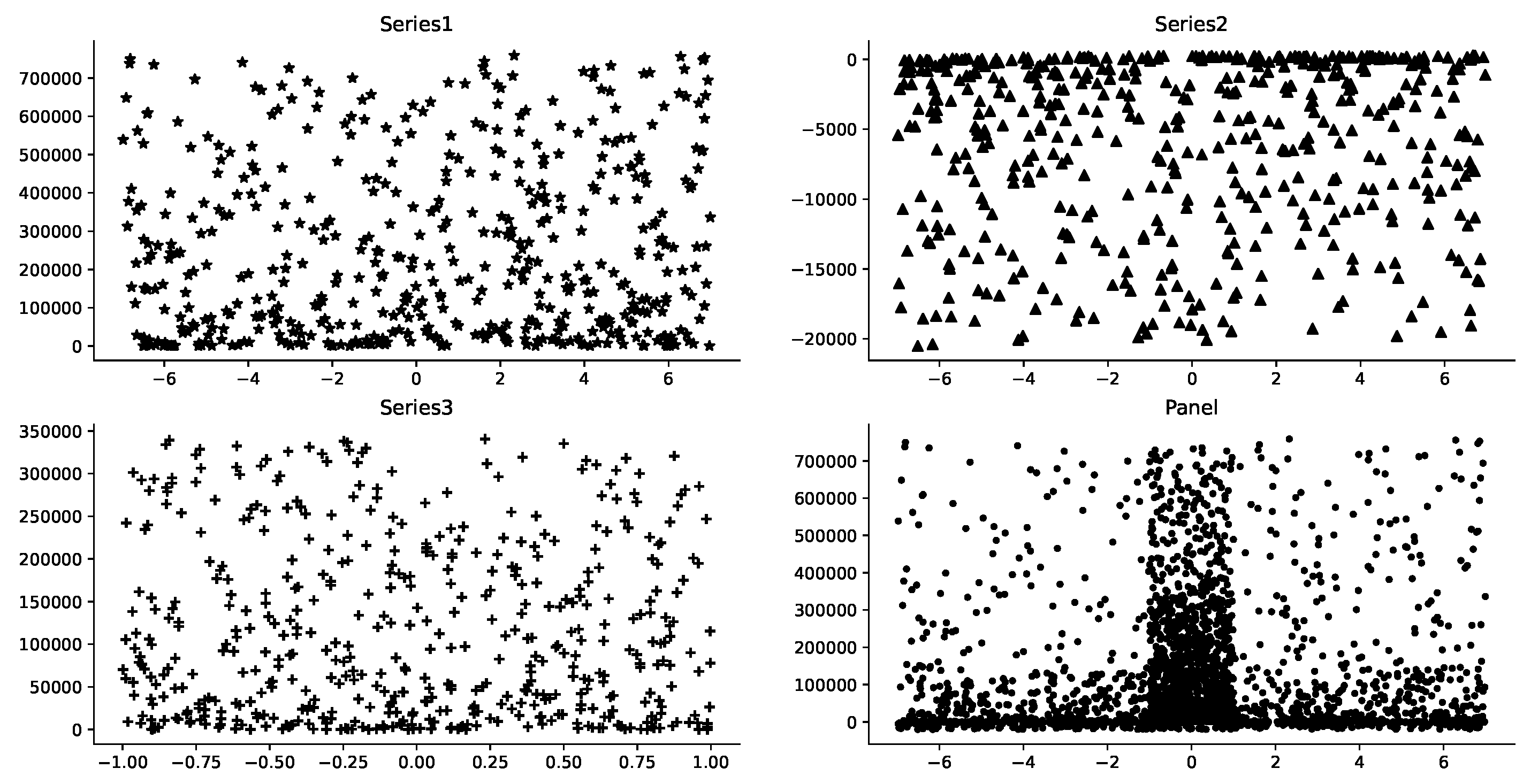
Downloads

90

Views

35

Comments

0

This version is not peer-reviewed

Submitted:

02 July 2024

Posted:

03 July 2024

You are already at the latest version

Alerts
Abstract
In economics, especially econometrics, fixed-effects are widely recognized as powerful tools for heterogeneity analysis of longitudinal data sets. However, the existing research pays more attention to such as the variable selection, parameter estimation and dimension reduction on linear relationships with too many assumptions while nonlinear relationships are ubiquitous. In this paper, an extension fixed-effects model is proposed on the curve_fit nonlinear least squares. First, with the help of expert knowledge, the series regressions between independent variables including time and dependent variable is estimated on each series data, and the parameters are estimated by curve_fit. Similarly, the coeffection between independent variables including time and dependent variable is also initially estimated on the whole panel data. Second, the distance between regressions is defined, and then the coeffect function between the series regressions is obtained on the initial co-effect with curve_fit. Third, the time-effects and individual fixed-effects for each series data in the panel data are estimated on the differences of series regressions and co-effect function. Additionally, the effectiveness of the proposed method is varified on the synthetic data.
Keywords: 
Subject: Business, Economics and Management  -   Econometrics and Statistics

1. Introduction

The panel data over both cross-section and time series gives users the possibility of accounting for multiple sources of unobserved heterogeneity in economics especially econometrics and statistics. Model formulations in which individual and/or time heterogeneity factors are considered fixed parameters than random variables, are called fixed-effects model [1]. The commonality (i.e., coeffect) of the distribution characteristics of time series datas can reflect the overall trend of the panel data, which is affected by independent variables including time respectively. In general, if the influence of time on the distribution of panel data satisfies certain rules, it is considered that there is time-effect in the distribution of the panel data. After removing the coeffect from the panel data, if the distribution of a time series data satisfies a certain rule, it is considered that the time series data in the panel data satisfies individual fixed-effect. Time-effects and individual fixed-effects are collectively called two-way fixed-effects or fixed-effects. Sometimes, fixed-effects in the narrow sense refer to individual fixed-effects.

1.1. Basic Definitions and Methods

There are some assumptions on the classical definitions of fixed-effects[2]. First, all time series datas distribute in linear with same slope(or slopes) between the independent variable(or variables) except the time and the dependent variable(or variables). Second, if there is a time fixed-effect in the panel data, the time fixed-effect is relatively independent and has nothing to do with other independent variables. Third, if there is an individual fixed-effect in the panel data, it is either relatively independent and has nothing to do with any independent variable beside the time (i.e., random-effects) or with some independent variables(i.e., narrow fixed-effects). Moreover, if all the time series have the same slope and intercept, some scholars call them mixed-effects. Besides, random-effects and mixed-effects are thought to be generalized fixed-effects [3]. In this paper, fixed-effects refer to fixed-effects in a broad sense. Therefore, functional expressions for fixed-effects differ in the number of dependent variables, and then they exist in two basic forms.The one form is single independent (i.e., input) variable beside the time with single dependent(i.e., output) variable. The other form is multiple independent variables beside the time with single dependent variable.
In the subsection, the random-effects are taken as an example to give the classical definitions and estimation method.
Definition 1. 
[4] Given the independent variables { x 1 , x 2 , , x k } where k N representing the count of independent variables. Let x i , j , t represent the value of x j for the i t h individual series in time t. Let y i , t be the value of dependent variable y for the i t h individual series in time t while ε i , t is the random residual error. Thus, the corresponding linear regression equation is shown below.
y i , t = j = 1 k ( β j × x i , j , t + α j ) + u i + v t + ε i , t
In the equation 1, all time series datas share the same slope β j with the same intercept α j for the independent variable x j . Meanwhile, the individual fixed-effect u i changes with individual i, but remains internally consistent for the same time series data. Similarly, the time fixed-effect v t changes with the time t, but remains internally consistent for the same cross-section data.
Since y i , t and x i , j , t have been given by a panel data for each i, j and t, the parameters like α j , β j , u i and v t should be estimated with a residual ε i , t as small as possible to check whether there are individual fixed-effects (i.e., u i ) and time fixed-effect (i.e., v t ). Let the time cycle be from 1 to τ (i.e., t { 1 , 2 , , τ } ). Therefore, there are three main methods to estimate parameters such as fixed-effects transformation, dummy variable, first difference, Monte Carlo simulation and so on [5]. For example, the fixed-effects transformation is as following.
y i , t y i ¯ = ( j = 1 k ( β j × x i , j , t + α j ) + u i + v t + ε i , t ) ( t = 1 τ j = 1 k ( β j × x i , j , t + α j ) + u i + v t + ε i , t ) ) / τ = j = 1 k ( β j × ( x i , j , t x i , j ¯ ) + ( α j α j ¯ ) ) + ( u i u i ¯ ) + ( v t t = 1 τ v t ) + ( ε i , t t = 1 τ ε i , t / τ ) = j = 1 k ( β j × ( x i , j , t x i , j ¯ ) ) + ( v t t = 1 τ v t ) + ( ε i , t ε i ¯ )
In equation 2, the individual fixed-effects variable u i can be eliminated as the fixed-effect of each individual doesn’t change with the time (i.e., u i = u i ¯ ). Let y i , t y i ¯ = y ¨ i , t , x i , j , t x i , j ¯ = x ¨ i , j , t , v t t = 1 τ v t = v ¨ i , t , ε i , t ε i ¯ = ε ¨ i , t . Thus, the equation 2 can be changed as
y ¨ i , t = j = 1 k ( β j × ( y ¨ ) i , t ) + v ¨ i , t + ε ¨ i , t
Furthermore, the parameters in the equation 3 can be estimated by the mixed Ordinary Least-Squares regression (i.e., OLS) [6].

1.2. Related Works

In order to meet the application needs of economics, management and other disciplines, the fixed-effect model has been continuously expanded and deepened. Since the count of independent variables get to be larger and larger, Correia et al. [7] propose a new command for estimation of (pseudo-)Poisson regression models with multiple high-dimensional fixed-effects. Similarly, sufficient dimension reduction is used for fixed-effects anylysis [8]. Meanwhile, meta analysis also works on fixed-effects [9]. On the contrary, some datas(i.e., long panels) have long time periods, Fernández-Val Iván and Weidner Martin focus on semiparametric models with unobserved individual and time-effects [10] while short time is also mentioned [11]. As fixed-effects anylysis must work on data, repeated measures data, unmeasured confounding data, and others are noticed and resolved [12,13]. Moreover, lagged periods are sued in dynamic fixed-effects modeling for that the effects of variables may be cross-period [14,15]. With the advent of the era of artificial intelligence, algorithms such as LASSO, tree-structured clustering, DNN, LSTM, multimodal, Bayesian and so on have been introduced to improve fixed-effects analysis [16,17,18,19,20,21]. However, major of fixed-effects analysis methods assumes that the panel data distributes in linear while nonlinear relationships are a common phenomenon in the real word [22]. In fact, fixed-effects in nonlinear is also be mentioned. William use Monte Carlo methods to examine the small sample bias in the binary probit and logit models, the ordered probit model, the tobit model, the Poisson regression model for count data and the exponential regression model for a nonnegative random variable [23]. Karyne investigates whether existing methods can be modified to eliminate multiple fixed-effects for some specific models in which the incidental parameter problem has already been solved in the presence of a single fixed-effect [24]. Irene and Chris discuss identification of counterfactual parameters in a class of nonlinear semiparametric panel models with fixed-effects and arbitrary time-effects [25], but it needs to derive bounds of time-stationarity. In order to better explain causality, the explainability of fixed-effects is hotly debated [26,27]. Although Monte Carlo methods sometimes work well in the nonlinear panel data, the interpretability of the relationship between process and outcome is open to question. Additionally, existing nonlinear fixed-effect models work on logistic regression but not others like polynomial regression.

1.3. Main Contributions

To sum up, existing fixed-effects methods have three distinct restrictions at least. Most importantly, nonlinear relationships beside logistic regression are common in the real world, but not covered by existing methods. Additionally, expert knowledge is not fully utilized in the fixed-effects analysis and only exists in the form of preliminary judgments. In other words, experts only preliminarily judge whether there may be fixed-effects and rely on ready-made models for verification, but do not use their professional knowledge to intervene in the verification of fixed-effects models. Furthermore, time-effects do not eliminate the coeffect of time on the panel data as a whole, that is, the time-effects fail to reflect heterogeneity.
In this paper, an extension fixed-effects model is proposed on the curve_fit nonlinear least squares based on the expert knowledge.
  • First, the regressions between independent variables including time and dependent variable is estimated on each time series data, and the parameters are estimated by curve_fit. Experts should guess the distribution functions between independent variables and the dependent variable based on professional theory and experience. The functions can be linear, which can be thought of as specially nonlinear, or they can be nonlinear. Users follow curve_fit to verify the matching degree of the functions until satisfied, otherwise adjust the functions. Similarly, the coeffect of the whole panel data is also initially estimated.
  • Second, the distance between regressions is defined, and then the coeffect function between the series regressions is obtained on the initial co-effect with curve_fit. Series regressions may be affected by coeffect in panel data, which reflects the commonality of these functions in distributions. To find coeffect functions that minimizes the sum of the squares of the average distance from each series sub-function as the common function. Thus, curve_fitting method is improved for the co-effect finding.
  • Third, the time-effects and individual fixed-effects for each series data in the panel data are estimated on the differences of series regressions and coeffect function. However, coeffect may be affected by time or other independent variables, which may cause bias in the analysis. Thus, We divide each regression into two sub-functions according to time and other independent variables. By eliminating the coeffect in series regressions, new individual fixed-effect and time-effect are obtained to better reflect the heterogeneity.
  • Additionally, the effectiveness of the proposed method is varified on the synthetic data. The method of verifying the validity of the classical model is usually based on expert knowledge and lacks objective metrics. This paper generates synthetic data based on the theory of fixed-effects, and determines the validity of model estimation by comparing the similarity between the expected fixed-effects and the estimated fixed-effects.
Therefore, there are three main contributions in our works.
(1)
First of all, the nonlinear relationships which generally exist in the real world are reflected by nonlinear functions, so that the fixed-effects model can be effectively extended at the application level.
(2)
Secondly, the prior knowledge of experts is fully utilized in the proposed fixed-effects analysis through the estimation function to prevent the separation of theory and empirical research, so that the model has better interpretability and is easier to be understood.
(3)
Thirdly, the proposed time-effects eliminate the coeffect of time in panel data, which can more effectively reflect the heterogeneity of time series datas in time distribution. Finally, individual fixed-effects can be either correlated or uncorrelated with independent variables, avoiding the distinction between fixed-effects and random effects.
(4)
In addition, based on synthetic data, a method to verify the validity of the fixed-effects model is proposed.

2. Proposed Method

2.1. Redefinition

In order to highlight the research topic, this paper does not discuss the endogeneity of variables and latent variables, and assumes that the selection of independent and dependent variables is reasonable. Given a pannel data P d over cross-section and time series datas with k independent variable vector X (i.e., { x 1 , x 2 , , x k } ) following by cross-section variable i ( i { 1 , 2 , , l } ) in time periods t ( t { 1 , 2 , , τ } , and the dependent variable y. Thus, x i , j , t represents the value of x j on the i t h series in time t. Meanwhile, y i , t means the value of y on the i t h series in time t.
It is assumed that in panel data P d , the distributions of P d follows certain rules (or characteristics) on time series with heterogeneity. First, regardless of the series datas, all data distribution in the panel data follows a coeffect y = f c ( X , t ) . Second, in the i t h time series data, the data distributions follow the function y i = f i ( X , t ) .
Definition 2. 
The differece f i c ( X , t ) between the i t h time series data distribution and the coeffect calls the fixed-effect of the i t h time series data in the panel data P d .
f i c ( X , t ) = f i ( X , t ) f c ( X , t )
If X and t are independent with each other in both f i ( X , t ) and f c ( X , t ) , f i ( X , t ) and f c ( X , t ) can be decomposed into f i ( X ) + g i ( t ) and f c ( X ) + g c ( t ) ,respectively. Namely,
f i ( X , t ) = f i ( X ) + g i ( t )
f c ( X , t ) = f c ( X ) + g c ( t )
Therefore, the equation 4 can be rewritten as
f i c ( X , t ) = ( f i ( X ) + g i ( t ) ) ( f c ( X ) + g c ( t ) ) = ( f i ( X ) f c ( X ) ) + ( g i ( t ) g c ( t ) )
If there is no appropriate function to fit the data distribution, the corresponding function can be 0 (i.e., false).
Since f c ( X ) represents the effect of X on y on panel data P d , which is generic. And f i ( X ) represents the effect of X on y on the i t h time series data. Thus, f i ( X ) f c ( X ) represents the personality effect of X on y on the i t h time series data. We call that
Definition 3. 
f i ( X ) f c ( X ) is the individual fixed-effect of the i t h series data on the panel data P d .
If f c ( X ) = 0 but f i ( X ) 0 , it means there is an absolute heterogeneiry (i.e., absolute individual fiexed-effect) affected by X in the i t h series data. Additionally, if f i ( X ) = 0 with most likely f c ( X ) = 0 because series stochasticity affected by X most likely leads to panel stochasticity affected by X, it means the series data is randomly distributed and the significance of heterogeneity affected by X (i.e., individual fixed-effect) is not explored. If f i ( X ) = f c ( X ) 0 , that is to say, the i t h series data distributes the same affected by X with the whole panel data. In other words, there is no heterogeneity affected by X (i.e., no individual fixed-effect) between the i t h series data and the panel data when f i ( X ) f c ( X ) = 0 .
i e i = F a l s e f i ( X ) = 0 o r f i ( X ) = f c ( X ) f i ( X ) f c ( X ) o t h e r s
where i e i represents the individual fixed-effect of the i t h series data in the the panel data.
Similarlly, because g i ( t ) represents the effect of t on y on panel data P d , which is generic. And g c ( t ) represents the effect of t on y on the i t h time series data. Thus, g i ( t ) g c ( t ) represents the personality effect of t on y on the i t h time series data. We call that
Definition 4. 
g i ( t ) g c ( t ) is the time-effect of the i t h series data on the panel data P d .
If g c ( t ) = 0 but g i ( t ) 0 , it means there is an absolute heterogeneiry affected by time t (i.e., absolute time-effect) in the i t h series data. Additionally, if g i ( t ) = 0 with most likely g c ( t ) = 0 because series stochasticity affected by t most likely leads to panel stochasticity affected by t, it means the series data is randomly distributed and the significance of heterogeneity affected by t (i.e., time-effect) is not explored. If g i ( t ) = g c ( t ) 0 , that is to say, the i t h series data distributes the same affected by t with the whole panel data. In other words, there is no heterogeneity affected by t (i.e., no time-effect) between the i t h series data and the panel data when g i ( t ) g c ( t ) = 0 .
t e i = F a l s e g i ( t ) = 0 o r g i ( t ) = g c ( t ) g i ( t ) g c ( t ) o t h e r s
where t e i represents the time-effect of the i t h series data in the the panel data.
Compared with the equation 1, it can be seen in the equation 7 that f i ( X ) , f c ( X ) , g i ( t ) , and g c ( t ) are undetermined. All of them can be either in linear or nonlinear, let alone with the same slope in time series data distributions. Furthermore, the time-effects are not only a function of the time period, but also the results of eliminating the ceffect of time on the panel data in time series datas. Obviously, in comparison with the classical time-effects, the conditions of time-effects in the denifition 4 are relaxed, and the commonality is no longer emphasized, but the individuality is highlighted, which is more in line with the purpose of fixed-effect analysis. In a word, the classical fixed-effects are extended.

2.2. Solutions

It is well known that when analyzing whether there are fixed-effects in a panel data, only the values of x i , j , t for each independent variable j ( i { 1 , 2 , , k } ) in each i t h ( i { 1 , 2 , , l } ) series data in the time period t ( i { 1 , 2 , , τ } ) are usually given without knowing the distribution functions.
Therefore, there are two main works should do. First, we need to know what type of distributions f i ( X ) , f c ( X ) , g i ( t ) , and g c ( t ) satisfy (e.g., polynomial distribution, linear distribution, or constants). Second, we need to estimate their parameters according to their distribution types, so as to realize the fixed-effects prediction. Of course, if there are no fixed-effects in the original panel data, such speculation and estimation should be proved not to be accepted. Otherwise, the model is invalid.
Since these functions (i.e., f i ( X ) , f c ( X ) , g i ( t ) , and g c ( t ) ) are curves in the pannel data over time series datas, curves fitting on the nonlinear least square is considered the main solution.

2.2.1. Curve Fitting

The idea of curve fitting is to find a mathematical model that fits a series of data points, possibly subject to constraints. It is assumed that users have theoretical reasons for picking a function of a certain form in general. The curve fitting finds the specific coefficients (parameters) which make that function match the data as closely as possible. In detail,raw data and a function with unknown coefficients are given in curve fitting. The main target is to find values for the coefficients such that the function matches the raw data as well as possible. The best values of the coefficients are the ones that minimize the value of chi-square. Chi-square is defined as
i ( f ( x i , θ ) y i σ i ) 2
where f ( x i , θ ) is a fitted value (model value) for a given point ( x i , y i ) on the function f with the estimated parameter vector θ . y i is the measured data value for x i and σ i is an estimate of the standard deviation for y i . In other words, for raw data points consisting of ( x i , y i ) , the minimum chi-square with the estimated parameter set θ for the given function f is expected. To get best paramters θ , nonlinear least square is used.
For the nonlinear built-in data fitting functions and for user-defined functions, the operation must be iterative. Igor tries various values for the unknown coefficients. For each try, it computes chisquare searching for the coefficient values that yield the minimum value of chi-square.
Given some initial guess of the parameter values θ = θ 0 , hold x i constant and form the first order Taylor approximation
f ( x i , θ ) y i [ ( f ( x i , θ 0 ) + d d θ f ( x i , θ ) | θ = θ 0 ( θ θ 0 ) ) ] y i [ f ( x i , θ 0 ) + f θ ( x i , θ 0 ) ( θ θ 0 ) ] y i [ f ( x i , θ 0 ) f θ ( x i , θ 0 ) θ 0 y i ] + f θ ( x i , θ 0 ) θ y i + f θ ( x i , θ 0 ) θ
and the nonlinear least square problem has become a linear least square promblem [28].

2.2.2. Detailed Steps

(1)Curves fitting in series datas
A panel data includes a group of time series datas. For each time series data, the industry expert can give a function to describe the data distribution between independent variables including time period and dependent variable according to their prior knowledge. First, the distribution type of the function marked as ψ i ( θ i ) can be guessed based on the theoretical knowledge held by the expert where ψ i ( θ i ) represents the funtion ψ i whose paramter vector is θ i . For example, the threshold effect may be related to the sigmoid function, and that U-shaped curves usually correspond to quadratic functions. Second, the initial parameters ψ i can be guessed as ψ i 0 by the expert. Third, given the function ψ i ( θ i ) and initial parameters ψ i 0 , truth parameters can be estimated by the curve-fitting with the nonlinear least square following the equations 10 and 11. According to the equation 4, the ideal result is
ψ i ( θ i ) = f i ( X , t )
However, f i ( X , t ) is usually unknown. Thus, the smaller the residual(i.e., the equation 10), the better. If the residual is too big(e.g., greater than a give threshold), ψ i ( θ i ) should be adjusted to meet the requirements, or the fitting should be rejected if they are not satisfied after many adjustments.
Particularly, ψ i ( θ i ) can be either linear or nonlinear. That is to say, the functions satisfy the nonlinear leads an extension of curve fitting in classical fixed-effects analysis.
Similarly, if the time series data are mixed and the overall panel data distribution characteristics(marked ψ c ( θ c ) ) are estimated. The ideal result is
ψ c ( θ c ) = f c ( X , t )
as shown in the equation 4. The smaller the residual(i.e., the equation 10), the better. If the residual is too big(e.g., greater than a give threshold), ψ i ( θ c ) should be adjusted to meet the requirements, or the fitting should be rejected if they are not satisfied after many adjustments.
Therefore, if both ψ i ( θ i ) and ψ c ( θ c ) are acceptable, the heterogeneity(i.e., fixed-effect) of the i t h time series data in the panel data P d is
ψ i ( θ i ) ψ c ( θ c )
,or else the fixed-effect isn’t acceptable.
(2)Time-effects and individual fixed-effects estimate
If the independent variables and the time periods are independent of each other when there are fixed-effects in the panel data P d , separate ψ i ( θ i ) and ψ c ( θ c ) with time and other independent variables into two parts, namely,
ψ i ( θ i ) = ϕ i ( θ i t ) + ω i ( θ t )
where ϕ i ( θ i t ) fits the effects of independent variables except the time and ω i ( θ t ) fits the effects of time on the dependent variable in each series data.
Similarly,
ψ c ( θ c ) = ϕ c ( θ c t ) + ω c ( θ t )
where ϕ c ( θ c t ) fits the effects of independent variables except the time and ω c ( θ t ) fits the effects of time on the dependent variable in the global panel data.
Combining the equation 15 and 16 and comparing with the equation 7, we can see that the closer ϕ i ( θ i t ) , ω i ( θ t ) , ϕ c ( θ c t ) , ω c ( θ t ) are correspondingly to f i ( X ) , g i ( t ) ) , f c ( X ) , g c ( t ) , the better. Thus, following the equation 7, the time-effect of the i t h series data in the panel data can be initialized as
ω i ( θ t ) ω c ( θ t )
, and the corresponding individual fixed-effect can be initialized as
ϕ i ( θ i t ) ϕ c ( θ c t )
However, either ω c ( θ t ) or ϕ c ( θ c t ) may be offset by estimating together with other independent variables. In order to correct this bias, we use the principle of least squares to correct ω c ( θ t ) and ϕ c ( θ c t ) based on the loss function over the the function similarity. The loss function is defined as
i = 1 k t = 1 τ ( ω c ( θ t ) ω i ( θ t ) min ( ω c ( θ t ) , ω i ( θ t ) ) ) 2 k
instead of the equation 10. And then, the function with the best parameter vector for ω c ( θ t ) can be catched.
Similarly, the loss function is defined as
i = 1 k t = 1 τ ( ϕ c ( θ i t ) ϕ i ( θ i t ) min ( ϕ c ( θ i t ) , ϕ i ( θ i t ) ) 2 k
instead of the equation 10. And then, the function with the best parameter vector for ϕ c ( θ i t ) can be catched.
Along this line, the time-effects can be corrected as
ω i ( θ t ) ω c ( θ t )
, and the corresponding individual fixed-effect can be corrected as
ϕ i ( θ i t ) ϕ c ( θ c t )
If ω c ( θ t ) = 0 but ω i ( θ t ) 0 , it means there is an absolute heterogeneiry affected by time t (i.e., absolute time-effect) in the i t h series data. Additionally, if ω i ( θ t ) = 0 with most likely ω c ( θ t ) = 0 because series stochasticity affected by t most likely leads to panel stochasticity affected by t, it means the series data is randomly distributed and the significance of heterogeneity affected by t (i.e., time-effect) is not explored. If ω i ( θ t ) = ω c ( θ t ) 0 , that is to say, the i t h series data distributes the same affected by t with the whole panel data. In other words, there is no heterogeneity affected by t (i.e., no time-effect) between the i t h series data and the panel data when ω i ( θ t ) ω c ( θ t ) = 0 .
t e i = F a l s e ω i ( θ t ) = 0 o r ω i ( θ t ) = ω c ( θ t ) ω i ( θ t ) ω c ( θ t ) o t h e r s
where t e i represents the time-effect of the i t h series data in the the panel data.
If ϕ c ( θ c t ) = 0 but ϕ i ( θ i t ) 0 , it means there is an absolute heterogeneiry (i.e., absolute individual fiexed-effect) affected by X in the i t h series data. Additionally, if ϕ i ( θ i t ) = 0 with most likely ϕ c ( θ c t ) = 0 because series stochasticity affected by X most likely leads to panel stochasticity affected by X, it means the series data is randomly distributed and the significance of heterogeneity affected by X (i.e., individual fixed-effect) is not explored. If ϕ i ( θ i t ) = ϕ c ( θ c t ) 0 , that is to say, the i t h series data distributes the same affected by X with the whole panel data. In other words, there is no heterogeneity affected by X (i.e., no individual fixed-effect) between the i t h series data and the panel data when ϕ i ( θ i t ) ϕ c ( θ c t ) = 0 .
i e i = F a l s e ϕ i ( θ i t ) = 0 o r ϕ i ( θ i t ) = ϕ c ( θ c t ) ϕ i ( θ i t ) ϕ c ( θ c t ) o t h e r s
where i e i represents the individual fixed-effect of the i t h series data in the the panel data.

2.3. Algorithms

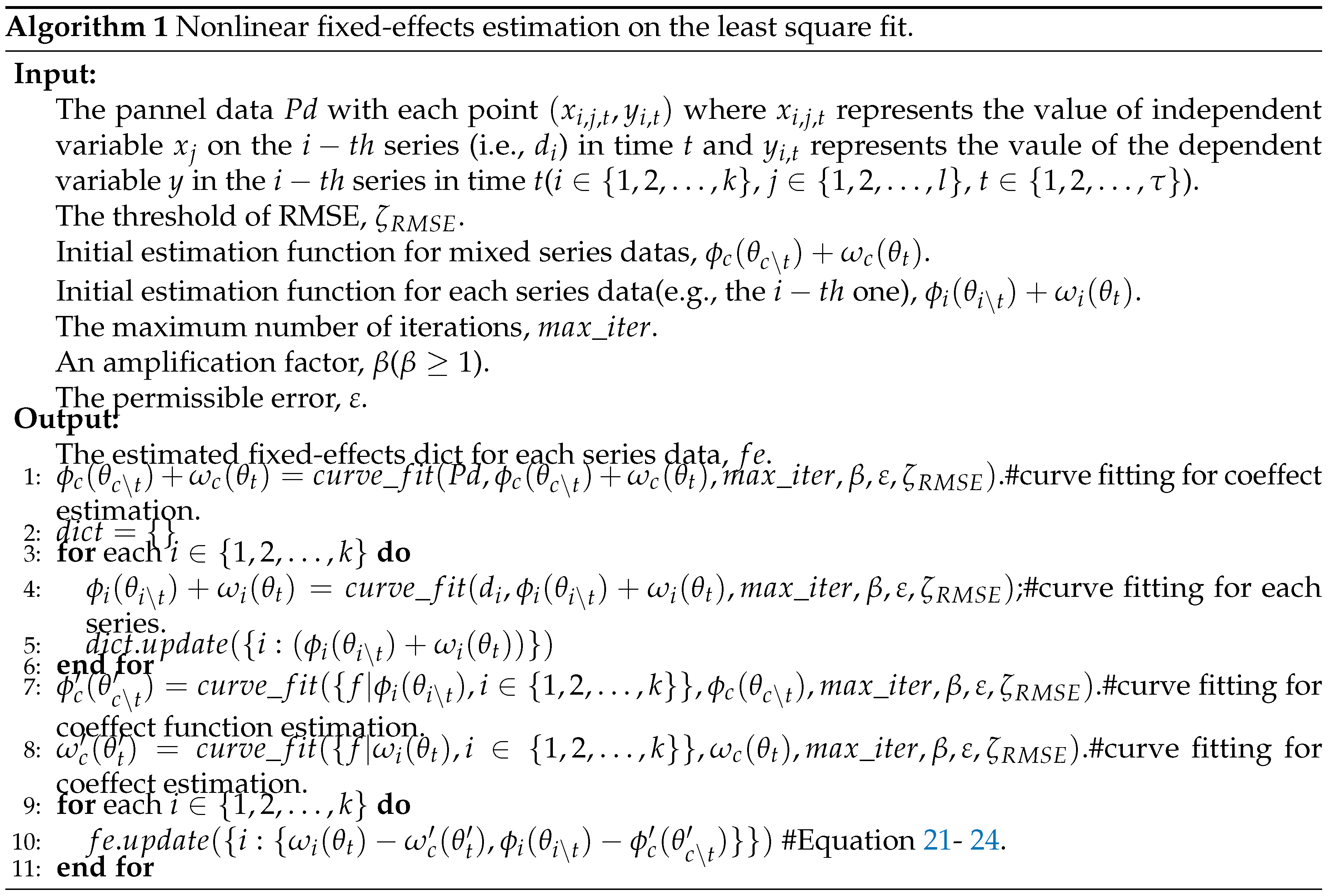
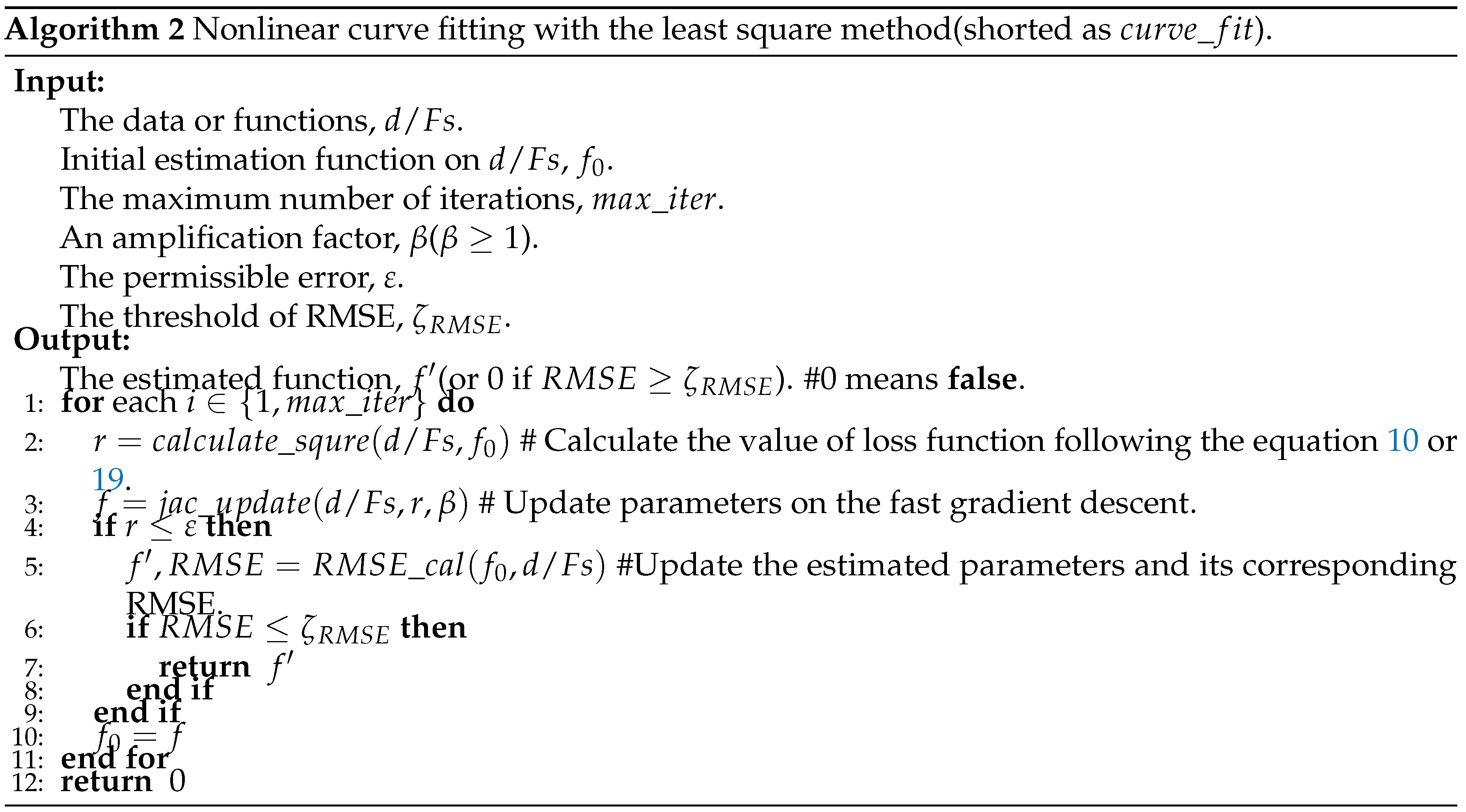
Based on the previous equations, this subsection gives the estimation algorithms (i.e., algorithm 1 and 2) of nonlinear fixed-effects. If there are time-effects or individual fixed-effects, their corresponding expressions are given, or not, false is given correspondingly. Preprints 110978 i001Preprints 110978 i002
Since each algorithm has been clearly commented, the detailed steps of the algorithm will not be explained separately in this section. If readers have any questions, please contact the corresponding author and request the corresponding codes.
Algorithm 1 fits each series data based on Algorithm 2 and returns the fitting results. If a fitting accepts, it returns the function; otherwise, it returns 0. According to time and other independent variables, the fitting functions are split to distinguish time-effects from individual fixed-effects. And then, the initial coeffect is fitted on the overall panel data. The fitting function of each series data takes the initial coeffect as the starting point and corrects the deviation of their coeffect functions. Finally, the individual fixed-effects and the time-effects are estimated as the differences between the series functions and the coeffect functions.

3. Experimental Results

In this section, to verify the validity of the proposed model, we generate synthetic data on the given functions and use the proposed model to verify the similarity between the estimated functions and the given functions.

3.1. Data Synthesis

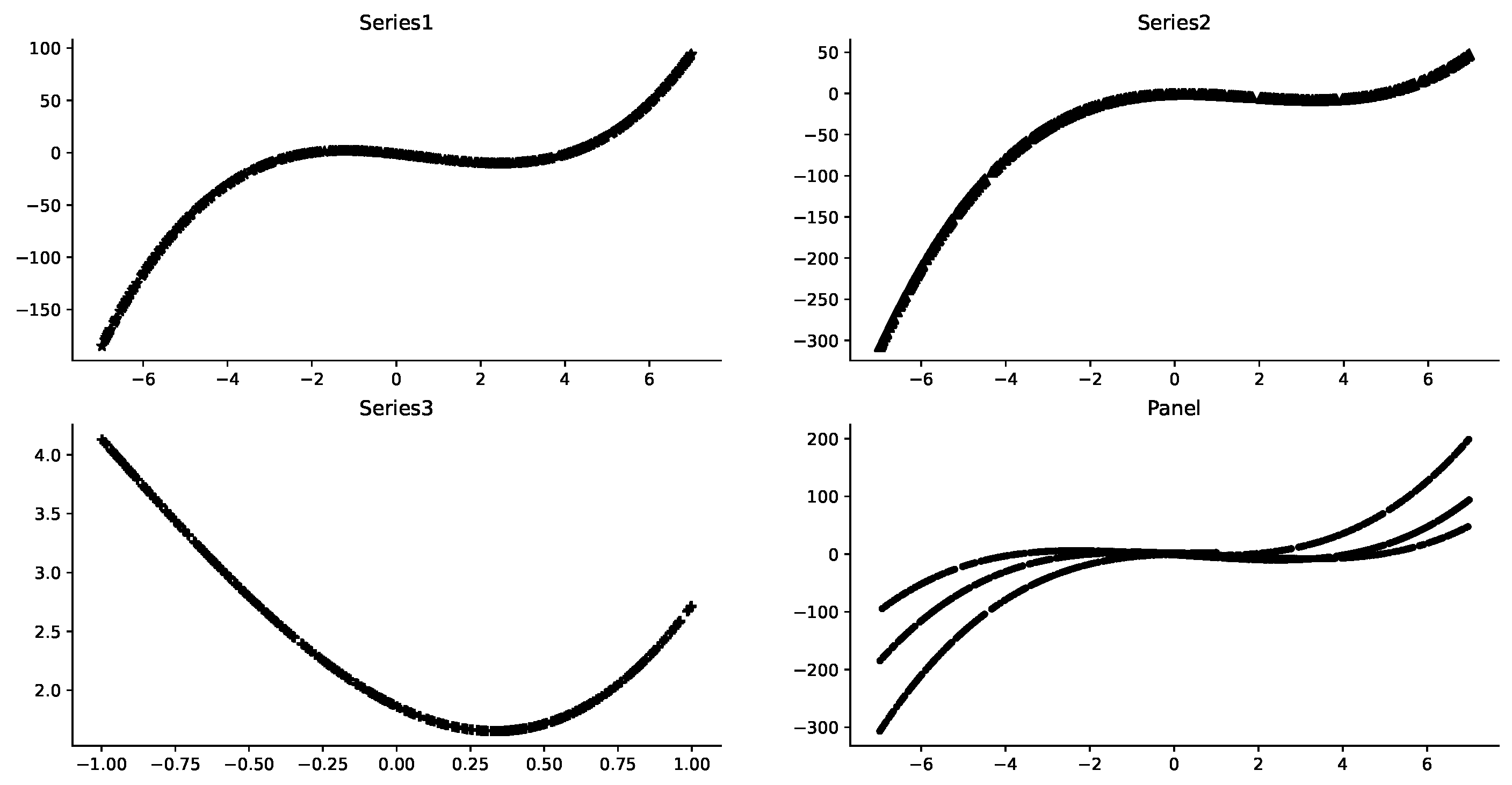
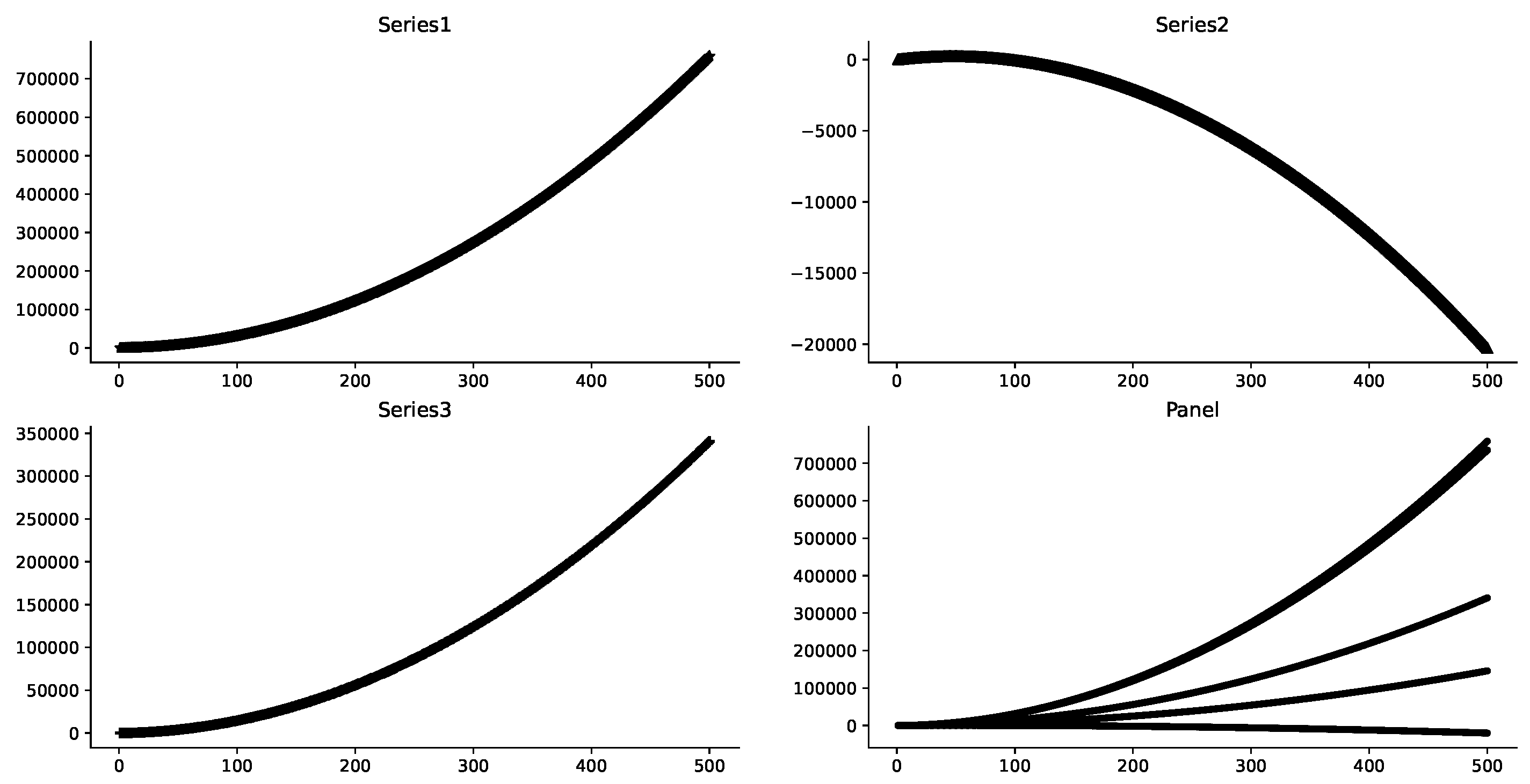
Following the equation 7, let f c ( X ) = 0.5 x 3 x 2 + 2 x 2 where the independent variable X is x( x [ γ , γ ] where γ is a random integer between 0 and 10 for each series data). Meanwhile, let g c ( t ) = 3 t 2 2 t + 7 where the time t is t( t { 1 , 2 , , 500 } ). Moreover, for each i t h ( i { 1 , 2 , 3 , 4 , 5 } , without loss of generality and easy to visualize, we use Series1, Series2, Series3, and Panel to correspondingly represent the fist, second, third and the whole panel datas.) series data, let f i ( X ) f c ( X ) = a x 2 + b x + c (i.e., the truth individual fixed-effect of the i t h series data on the panel data) and g i ( t ) g c ( t ) = d t 2 + e t + f (i.e., the truth time-effect of the i t h series data on the panel data) where a , b , c , d , e , f are random numbers in [-3,3],[-7,7],[-5,5],[-4,2],[11,19],[-3,6], correspondingly. Therefore, corresponding to the equation 4, for each i t h series data, f i ( X , t ) = 0.5 x 3 + ( a 1 ) x 2 + ( b + 2 ) x + ( 3 + d ) t 2 + ( e 2 ) t + c + f + 5 and f c ( X , t ) = 0.5 x 3 x 2 + 2 x + 3 t 2 2 t + 5 . In order to make the data closer to the real state of reality, random numbers between 0.00003 and 0.01 are added for perturbation to form the residuals of the fitted data. Thus, f i ( X , t ) = 0.5 x 3 + ( a 1 ) x 2 + ( b + 2 ) x + ( 3 + d ) t 2 + ( e 2 ) t + c + f + 5 + ε i , t where ε i , t is the random residual.
If fixed-effects are estimated using the classical model, the results are shown in Figure 1. It can be seen from Figure 1 that the classical model considers that there are both time-effect (Time) and individual fixed-effect (Entity) on a given data set. However, by observing its parameters, it can be seen that it is 832X+13210, which is far from the real value. Therefore, it can be argued that the existence of individual fixed-effects on a given data set should not be accepted.
It can be seen from Figure 2 that the representative series data show obvious characteristics of third-order polynomial distribution affected by x, as well as the overall data distribution. However, on the overall data, it is difficult to find a common third-order polynomial distribution function to fit them. Therefore, it is reasonable to assume that there are individual fixed-effects in each series data.
Similarly, it can be seen from Figure 3 that, affected by time t, the representative series data show obvious characteristics of second-order polynomial distribution, as well as the overall data distribution. However, on the overall data, it is difficult to find a common second-order polynomial distribution function to fit them. Therefore, it is reasonable to consider the existence of time-effect in each series data.

3.2. Data Distribution Observation

Figure 4 shows that it is difficult to observe how x alone affects the distribution of y when the effects of x and t on the data are mixed. In fact, it is equally difficult to observe the distributional impact of t on y. Similarly, in the subsequent results, it can also be found that it is very difficult to observe the influence of x and t on y at the same time.

3.3. Estimate Results

Fortunately, with the help of expert knowledge, it is assumed that x and y may satisfy a third-order polynomial distribution, and t and y may satisfy a second-order polynomial distribution, and they are independent of each other. Based on Algorithm 1, time-effects and individual fixed-effects are effectively estimated, and the results are shown in Table 1. At the same time, Table 1 also presents the estimation results based on the classical model. Obviously, the method in this paper is significantly better than the classical method.
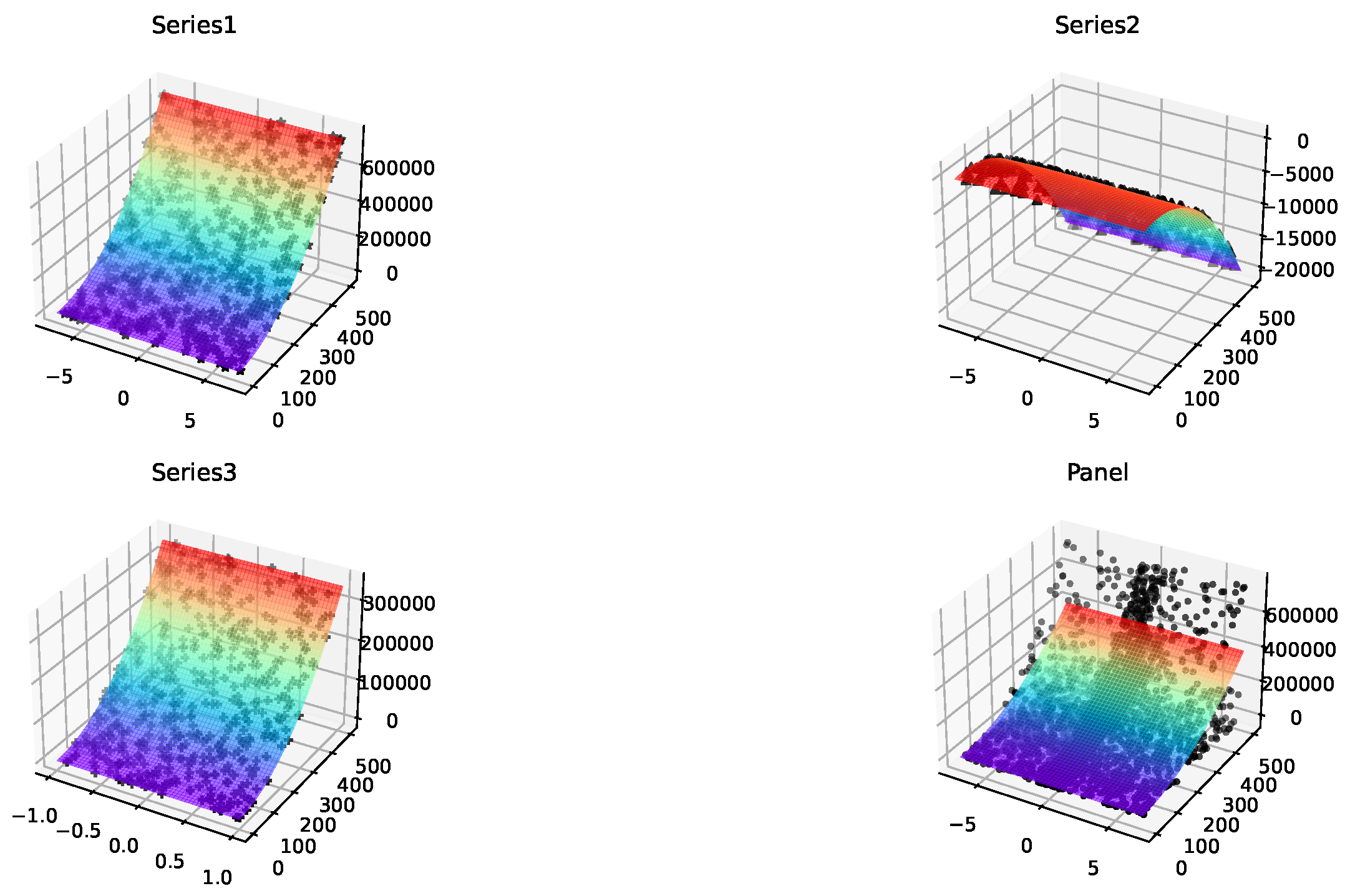
Perhaps the results given in Table 1 are not intuitive enough. Figure 5 shows the superiority of the method in this paper. It can be seen that the function fitting effects are particularly good on the three series datas, and the corresponding data points can be almost covered seamlessly. At the same time, the panel subfigure of Figure 5 shows that the estimated function can cover most of the data points, but not completely, which is the distribution adaptation with the synthetic data, precisely reflecting the heterogeneity among the serial datas.
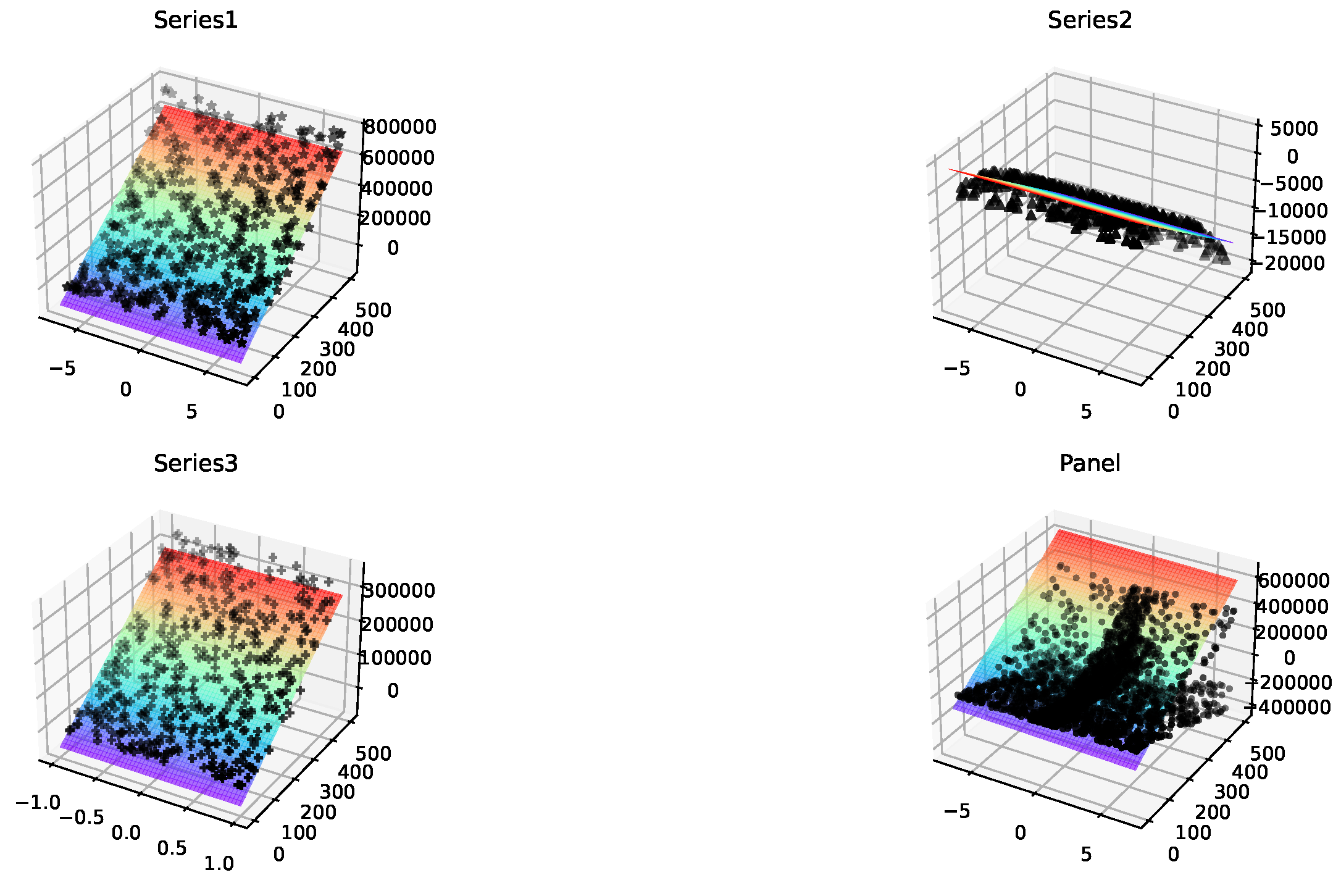
Figure 6 shows the fitting effects of the classical method on the three series data, showing that the fitting is not good and it is difficult to meet users’ expectations. Similarly, the fitting effect on the panel subgraph is not good. On the surface, heterogeneity among series data can be obtained. However, since the data fittings on the first three subgraphs are not effective, it is possible that this heterogeneity is caused by random distribution and should not be accepted.

4. Discussion and Conclusions

4.1. Discussion

Experiments show that, relying on expert knowledge and curve fitting, compared with the classical methods, the proposed method has better results in data fitting, and can better obtain the time-effects and individual fixed-effects on the synthetic data set, which is close to the real values. It can be seen that the result of fixed-effect verification depends on the accuracy of expert knowledge, and the higher the accuracy, the better the fitting effect. At the same time, the fitting algorithm also affects the results of verification, especially the new function fitting method can extend the data-based curve fitting to function fitting, and significantly improve the applicability of the algorithm. In addition, we also verify the results when the definition of fixed-effect is not met, and find that the classical method may incorrectly accept the existence of fixed-effect, while our method can better avoid this misjudgment.

4.2. Conclusions

In view of the fact that the classical models of fixed-effect analysis are mainly based on linear and logistic regression, without paying attention to the ubiquitous linear relationship, this paper proposes a nonlinear fixed-effect analysis model based on the least square method. Firstly, the model determines the type of data distribution (polynomial distribution or power distribution, etc.) based on expert knowledge, and gives the preliminary distribution function of each series data. Next, the parameters are effectively estimated by fitting the data based on the initial distribution function through the least squares method. Then, based on the loss function of least square method, the objective function of function fitting of multiple fitting functions is designed, and the fitted function is obtained. The differences between each series function and the fitted function are expressed as functions of the fixed-effects. If time and other independent variables are independent in the fitting function, then the fitting function is split according to time and other variables, and then the time-effect and individual fixed-effect are obtained by using similar methods. On the synthetic data set, the effect of our method is compared with that of the classical method. It is found that our method has significant advantages and can achieve the expected results. In addition, we found in the experiment that the fixed-effect can be rejected for the data that do not meet the fixed-effect.

4.3. Future Works

First of all, in the analysis of time-effect and individual fixed-effect, this paper assumes that time and other independent variables are independent of each other, while in reality they may be interdependent. Thus, relaxing this assumption is the focus of the future research. Secondly, there may be some problems in the judgment of complex data by expert knowledge. It is valueable to analyze how to minimize the unsatisfactory effect of data fitting in the case of lack of expert knowledge. Lastly, variable selection in nonlinear fixed-effect analysis and cross-period dynamic analysis are also directions for future consideration.

Author Contributions

Haitao Duan and Muquan Zou: Conceptualization, Investigation, Data Curation, Validation, Resources, Methodology, Formal analysis, Supervision, Writing - original draft, Writing - review. Jiankun Yang and Vanha Tran: Data Curation, Validation, Resources.

Funding

This work is supported by the Special Basic Cooperative Research Programs of Yunnan Provincial Undergraduate Universities Association (grant NO.202101BA070001-152,155), the National Natural Science Foundation of China (NSFC) (grant NO. 62066023, 62106024), the Humanities and Social Sciences Fund of the Ministry of Education of China (No. 23YJCZH262), the Caiyun Postdoctoral Program-Innovation Project of Yunnan Province, and the Scientific Research Project of Kunming University (No. XJZZ1706).

Institutional Review Board Statement

Not applicable.

Informed Consent Statement

Not applicable.

Data Availability Statement

For data, please contact the corresponding author.

Acknowledgments

Not applicable.

Conflicts of Interest

The authors declare no conflicts of interest.

References

  1. Balázsi, L.; Mátyás, L.; Wansbeek, T. , L., Ed.; Springer International Publishing: Cham, 2024; pp. 1–37. https://doi.org/10.1007/978-3-031-49849-7_1.Models. In The Econometrics of Multi-dimensional Panels: Theory and Applications; Matyas, L., Ed.; Springer International Publishing: Cham, 2024; Springer International Publishing: Cham, 2024; pp. 1–37. [Google Scholar] [CrossRef]
  2. Hill, T.D.; Davis, A.P.; Roos, J.M.; French, M.T. Limitations of Fixed-Effects Models for Panel Data. Sociological Perspectives 2020, 63, 357–369. [Google Scholar] [CrossRef]
  3. Broström, G.; Holmberg, H. Generalized linear models with clustered data: Fixed and random effects models. Computational Statistics and Data Analysis 2011, 55, 3123–3134. [Google Scholar] [CrossRef]
  4. Allison, P.D. Fixed effects regression models; SAGE publications, 2009.
  5. Lee, L.; Yu, J. Estimation of Spatial Panels; Foundations and trends in econometrics, Now, 2011.
  6. Craven, B.; Islam, S.M. Ordinary least-squares regression. The SAGE dictionary of quantitative management research.
  7. Correia, S.; Guimarães, P.; Zylkin, T. Fast Poisson estimation with high-dimensional fixed effects. The Stata Journal 2020, 20, 95–115. [Google Scholar] [CrossRef]
  8. Hui, F.; Nghiem, L. Sufficient dimension reduction for clustered data via finite mixture modelling. Australian & New Zealand Journal of Statistics 2022, 64, 133–157. [Google Scholar]
  9. Serghiou, S.; Goodman, S.N. Random-effects meta-analysis: summarizing evidence with caveats. Jama 2019, 321, 301–302. [Google Scholar] [CrossRef]
  10. Fernández-Val, I.; Weidner, M. Fixed effects estimation of large-T panel data models. Annual Review of Economics 2018, 10, 109–138. [Google Scholar] [CrossRef]
  11. Hsiao, C.; Pesaran, M.H.; Tahmiscioglu, A.K. Maximum likelihood estimation of fixed effects dynamic panel data models covering short time periods. Journal of econometrics 2002, 109, 107–150. [Google Scholar] [CrossRef]
  12. Oneal, J.R.; Russett, B. Clear and clean: The fixed effects of the liberal peace. International Organization 2001, 55, 469–485. [Google Scholar] [CrossRef]
  13. Gunasekara, F.I.; Richardson, K.; Carter, K.; Blakely, T. Fixed effects analysis of repeated measures data. International Journal of Epidemiology 2013, 43, 264–269. [Google Scholar] [CrossRef] [PubMed]
  14. Bai, J. Fixed-effects dynamic panel models, a factor analytical method. Econometrica 2013, 81, 285–314. [Google Scholar]
  15. Moon, H.R.; Weidner, M. Dynamic linear panel regression models with interactive fixed effects. Econometric Theory 2017, 33, 158–195. [Google Scholar] [CrossRef]
  16. Su, L.; Ju, G. Identifying latent grouped patterns in panel data models with interactive fixed effects. Journal of Econometrics 2018, 206, 554–573. [Google Scholar] [CrossRef]
  17. Berger, M.; Tutz, G. Tree-structured clustering in fixed effects models. Journal of computational and graphical statistics 2018, 27, 380–392. [Google Scholar] [CrossRef]
  18. Simchoni, G.; Rosset, S. Integrating random effects in deep neural networks. Journal of Machine Learning Research 2023, 24, 1–57. [Google Scholar]
  19. Golenvaux, N.; Alvarez, P.G.; Kiossou, H.S.; Schaus, P. An lstm approach to forecast migration using google trends. arXiv preprint arXiv:2005.09902, arXiv:2005.09902 2020.
  20. Marquart, L.; Haynes, M. Misspecification of multimodal random-effect distributions in logistic mixed models for panel survey data. Journal of the Royal Statistical Society Series A: Statistics in Society 2019, 182, 305–321. [Google Scholar] [CrossRef]
  21. Sadeghirad, B.; Foroutan, F.; Zoratti, M.J.; Busse, J.W.; Brignardello-Petersen, R.; Guyatt, G.; Thabane, L. Theory and practice of Bayesian and frequentist frameworks for network meta-analysis. BMJ Evidence-Based Medicine 2023, 28, 204–209. [Google Scholar] [CrossRef] [PubMed]
  22. Liao, Z.; Gu, Q.; Li, S.; Sun, Y. A knowledge transfer-based adaptive differential evolution for solving nonlinear equation systems. Knowledge-Based Systems 2023, 261, 110214. [Google Scholar] [CrossRef]
  23. Greene, W.H. The behavior of the fixed effects estimator in nonlinear models 2002. pp. 1–48.
  24. Charbonneau, K. Multiple fixed effects in nonlinear panel data models. Unpublished manuscript 2012. [Google Scholar]
  25. Botosaru, I.; Muris, C. Identification of time-varying counterfactual parameters in nonlinear panel models. Journal of Econometrics, 1056. [Google Scholar] [CrossRef]
  26. Xu, R. Measuring explained variation in linear mixed effects models. Statistics in medicine 2003, 22, 3527–3541. [Google Scholar] [CrossRef]
  27. Bell, A.; Jones, K. Explaining fixed effects: Random effects modeling of time-series cross-sectional and panel data. Political Science Research and Methods 2015, 3, 133–153. [Google Scholar] [CrossRef]
  28. Wu, Q.; Ying, Y.; Zhou, D.X. Learning Rates of Least-Square Regularized Regression. Foundations of Computational Mathematics 2006, 6, 171–192. [Google Scholar] [CrossRef]
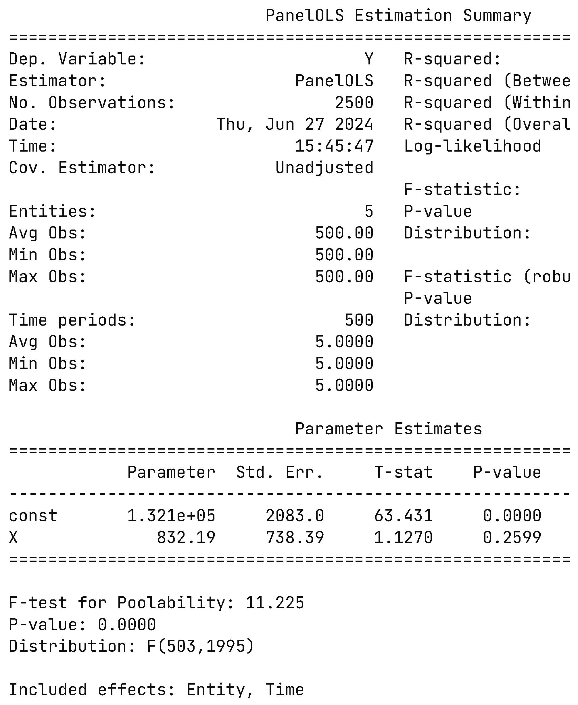
Figure 1. This is an example estimation summary on the panelOLS on the synthetic data. It shows that there are time-effects and individual fixed-effects. However, its parameter estimation results are far from the true parameter values.
Preprints 110978 g001
Figure 2. These are some data distributions of f i ( x ) = 0.5 x 3 + ( a 1 ) x 2 + ( b + 2 ) x + c 2 where the abscissas are x, and the ordinates are f i ( x ) . The values of a, b, c are random numbers(e.g., a = 0.085 in Series1).
Preprints 110978 g002
Figure 3. These are some data distributions of g i ( t ) = ( 3 + d ) t 2 + ( e 2 ) t + f + 7 where the abscissas are t, and the ordinates are g i ( t ) . The values of d, e, f are random numbers(e.g., e = 17.14 in Series1).
Preprints 110978 g003
Figure 4. These are some data distributions of f i ( X , t ) = 0.5 x 3 + ( a 1 ) x 2 + ( b + 2 ) x + ( 3 + d ) t 2 + ( e 2 ) t + c + f + 5 + ε i , t where the abscissas are x, and the ordinates are f i ( X , t ) . The values of a, b, c are random numbers(e.g., b = 0.95 in Series2)
Preprints 110978 g004
Figure 5. These are partial data set fit renderings of the proposed nonlinear model, where the left abscissas are x, the right abscissas are t, and the ordinates are f i ( X , t ) .
Preprints 110978 g005
Figure 6. These are partial data set fit renderings of the linear model, where the left abscissas are x, the right abscissas are t, and the ordinates are f i ( X , t ) .
Preprints 110978 g006
Table 1. This is a partial result of time-effects and individual fixed-effects on the synthetic data. Since it is difficult to distinguish whether the fitted intercepts belong to the time-effects or the individual fixed-effects, we attribute the intercepts to the time-effect in the proposed model, and to the individual fixed-effects in the classical model.
Fixed-effects Series data 1 Series data 2 Series data 3 Panel data(Coeffect)
]3*Time-effects 0.004 t 2 + 17.14 t + 2.85 3.10 t 2 + 11.59 t 2.20 1.66 t 2 + 14.07 t 2.71 3 t 2 2 t + 7
0.16 t 2 + 15.14 + 8.48 * 2.64 t 2 3.53 t + 4.15 * 0.20 t 2 1.05 t + 0.39 * 1.54 t 2 + 13.12 t + 5.76 *
61299.48 t ** 6880.90 t ** 8571.84 t ** 6.656 . 23 t **
]3*Individual fixed-effect 0.085 x 2 6.42 x + 0.63 1.64 x 2 0.95 x + 1.35 2.578 x 2 3.21 x + 3.868 0.5 x 3 x 2 + 2 x 2
0.08 x 2 2.95 x * 1.61 x 2 0.52 x * 2.54 x 2 + 0.36 x * 0.50 x 3 0.97 x 2 1.57 x *
21.9913 x + 1520.48 ** 2153.08 x 40.60 ** 3553.47 x + 682.47 ** 2155.12 x + 43.28 **
* The data is the result on the proposed nonlinear method.
Disclaimer/Publisher’s Note: The statements, opinions and data contained in all publications are solely those of the individual author(s) and contributor(s) and not of MDPI and/or the editor(s). MDPI and/or the editor(s) disclaim responsibility for any injury to people or property resulting from any ideas, methods, instructions or products referred to in the content.
Copyright: This open access article is published under a Creative Commons CC BY 4.0 license, which permit the free download, distribution, and reuse, provided that the author and preprint are cited in any reuse.
Prerpints.org logo

Preprints.org is a free preprint server supported by MDPI in Basel, Switzerland.

Subscribe

© 2024 MDPI (Basel, Switzerland) unless otherwise stated