Evaluating EEG-Based Parameters for Bipolar Disorder Diagnosis Using a Synthetic Dataset

1. Introduction

Electroencephalography (EEG) has a rich history dating back to the early 20th century when Dr. Hans Berger first demonstrated the presence of electrical activity in the human brain. Berger's discovery of "alpha waves" and "beta waves" laid the foundation for EEG as a critical tool in neuroscience and clinical diagnostics (Berger, 1929). Subsequently, significant advancements were made by researchers such as Dr. Wilder Penfield and Dr. Herbert Jasper, who mapped brain functions through direct electrical stimulation, enhancing the understanding of brain wave activities and their clinical implications (Penfield & Jasper, 1954); (Montgomery, R. M., 2024)

Recent studies have continued to build on this foundational work, exploring the applications of EEG in various neurological and psychiatric conditions. For instance, Montgomery et al. (2023) have discussed the evolution of EEG technology and its expanding role in neuropsychiatry, highlighting the improved sensitivity and versatility of modern EEG systems. Moreover, Montgomery's (2024*) review on advances in EEG technology emphasizes the importance of EEG's accessibility and cost-effectiveness in clinical practice, making it an ideal tool for widespread use in diagnosing conditions like bipolar disorder.

Section 1.1. Technological Advancements

EEG technology has evolved dramatically since its inception. Early EEG machines were limited by the technology of the time, offering low resolution and few electrodes. These systems were primarily used for diagnosing epilepsy due to their ability to detect the broad, distinctive electrical patterns associated with epileptic seizures. However, modern EEG systems have benefited from advancements in digital signal processing, electrode technology, and computational power. Today's EEG systems can capture high-resolution data from up to 256 channels, significantly improving spatial resolution and the ability to detect nuanced brain activity patterns (Niedermeyer & da Silva, 2004).

Section 1.2 Transition to Psychiatry

The enhanced capabilities of modern EEG have led to its expanded use in neuropsychiatry. Improved sensitivity, affordability, and unparalleled temporal resolution make EEG a valuable tool for diagnosing a variety of psychiatric conditions, such as schizophrenia, depression, ADHD, and bipolar disorder. EEG's real-time monitoring capabilities provide insights into the functional abnormalities underlying these disorders (Nuwer, 1997). Montgomery (2023) further explores the use of EEG in autism spectrum disorder, demonstrating how altered neural connectivity can be effectively studied using advanced EEG techniques.

Comparatively, functional Magnetic Resonance Imaging (fMRI) offers excellent spatial resolution but lacks the temporal precision of EEG. While fMRI can pinpoint where brain activity occurs, it cannot accurately capture the timing of neural events. This is akin to the police arriving at a crime scene five days after the event, whereas EEG provides a real-time account, capturing the immediate electrical activity of the brain as it happens (Pfurtscheller & da Silva, 1999). We have to be careful and fear the temptation to adopt Neo-Phrenology practices.

2. Methodology

2.1. Data Generation and Parameters

In this study, we generated a synthetic EEG dataset to evaluate the effectiveness of EEG-based parameters for diagnosing bipolar disorder. The dataset included both correctly diagnosed and misdiagnosed cases to simulate realistic clinical conditions. The following EEG parameters were used, as they are the most common and widely recognized in the literature:

Theta-Alpha Mean and Standard Deviation: Captures the average and variability in the voltage of theta and alpha waves.

Frontal Alpha Asymmetry Mean and Standard Deviation: Measures the differences in alpha wave activity between the left and right frontal lobes.

Beta Band Mean and Standard Deviation: Represents the average and variability in beta wave activity.

Event-Related Potentials (ERP) Mean and Standard Deviation: Measures the voltage changes in response to specific stimuli.

Coherence Mean and Standard Deviation: Assesses the synchronization between different brain regions.

Microstates Mean and Standard Deviation: Captures the temporal dynamics of brief, stable states of brain activity.

Nonlinear Dynamics Mean and Standard Deviation: Represents the complexity and variability in brain activity patterns.

These parameters were selected due to their widespread use in EEG research and their relevance in identifying neuropsychiatric conditions. The dataset was generated using a standard EEG configuration with 19 channels, based on the 10-20 system, which is commonly used in clinical practice.

Number of EEGs and Mixing

For this study, we generated a total of 200 synthetic EEG recordings, comprising both non-bipolar and bipolar cases to simulate realistic clinical conditions. The dataset was divided as follows:

• Non-Bipolar Cases:

Correctly Diagnosed: 90 EEGs generated with parameters typical for non-bipolar individuals.

Misdiagnosed as Bipolar: 10 EEGs generated with parameters typical for bipolar individuals but labeled (at a virtual anamnesis) as non-bipolar to simulate false positives.

2.

Bipolar Cases:

Correctly Diagnosed: 90 EEGs generated with parameters typical for bipolar individuals.

Misdiagnosed as Non-Bipolar: 10 EEGs generated with parameters typical for non-bipolar individuals but labeled as bipolar to simulate false negatives.

Data Preparation and Model Training

Dataframe Creation:

Combined the non-bipolar and bipolar EEG recordings into a single dataframe.

Assigned labels: 0 for non-bipolar and 1 for bipolar.

Data Splitting:

Split the combined dataset into training (80%) and testing (20%) sets using stratified sampling to maintain the class distribution.

Standardization:

Standardized the features using StandardScaler to ensure each feature had a mean of 0 and a standard deviation of 1.

Model Architecture:

Constructed a multi-layer perceptron (MLP) model with the following architecture:

Input layer with 128 neurons and ReLU activation.

Hidden layers with 64, 32, 16, 8, and 4 neurons, each using ReLU activation.

Output layer with a single neuron and sigmoid activation for binary classification.

Model Compilation and Training:

Compile the model using the Adam optimizer, binary cross-entropy loss, and accuracy as the metric.

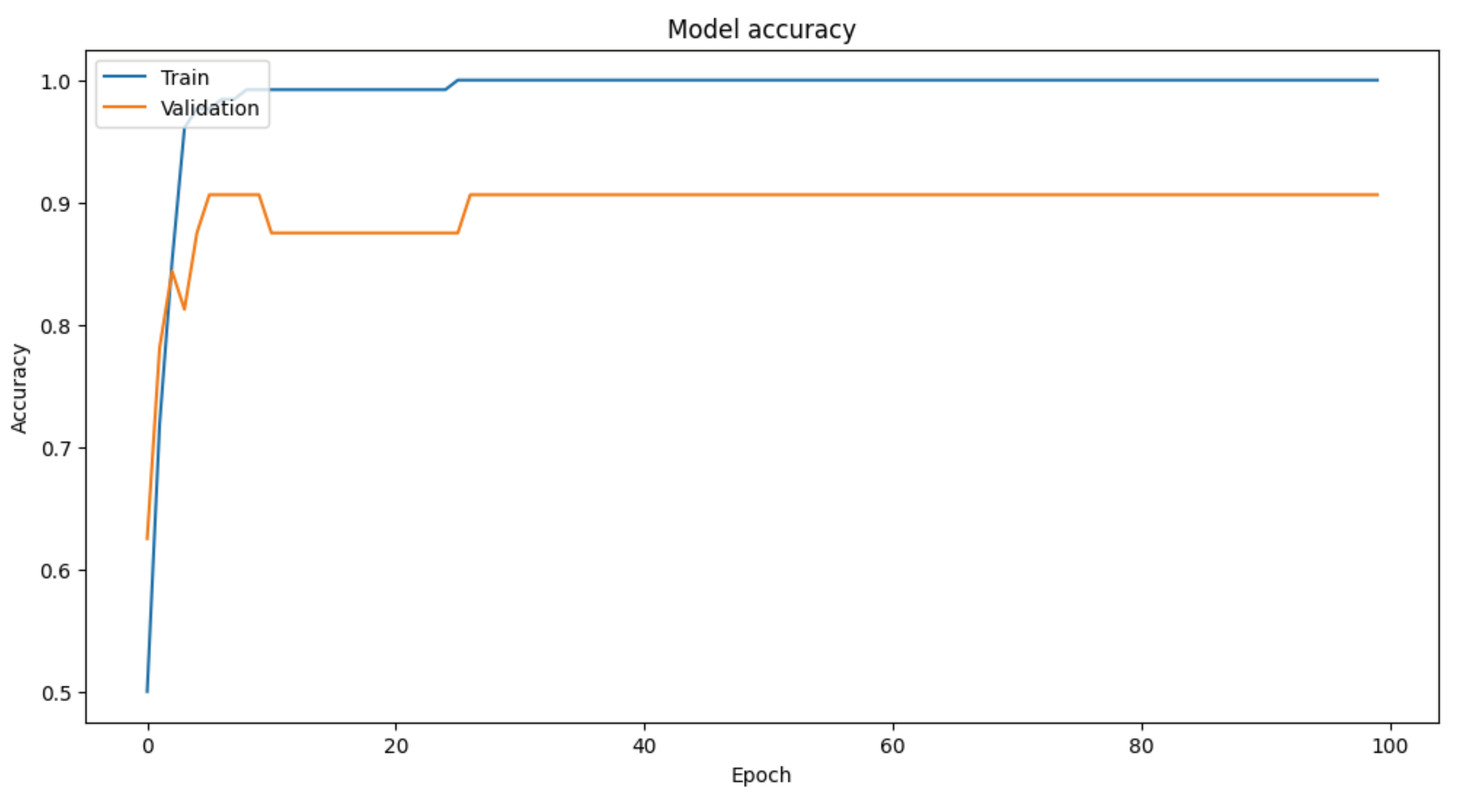
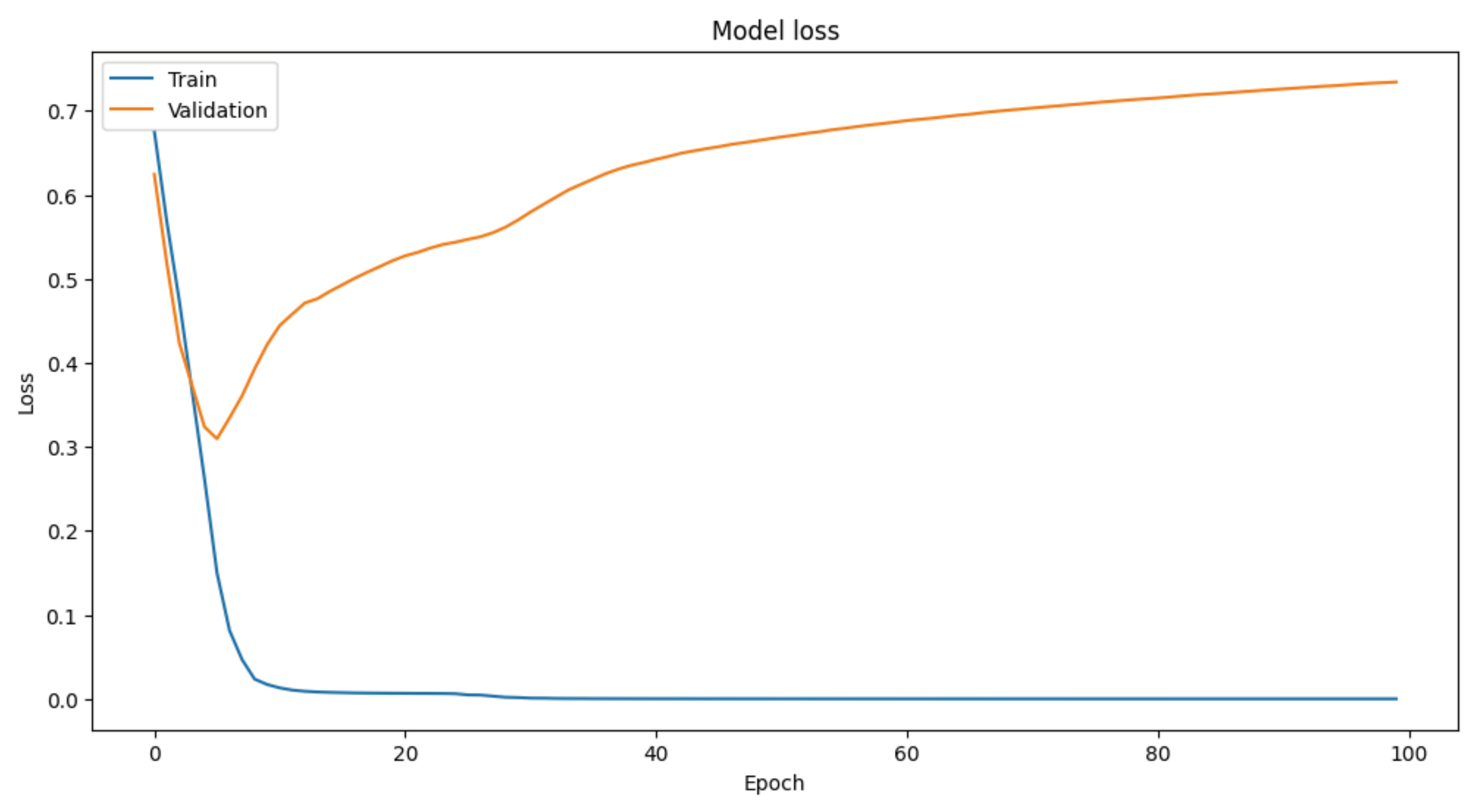
Trained the model for 100 epochs with a batch size of 16 and a validation split of 20%.

2.2. Model Evaluation

Evaluated the model's performance on the test set, achieving a test accuracy of 92%.

This methodology demonstrates the feasibility of using synthetic EEG data to train machine learning models for diagnosing bipolar disorder. The selected EEG parameters, combined with robust data preparation and model training techniques, yielded high diagnostic accuracy, underscoring the potential of EEG-based diagnostics in neuropsychiatry. Of course, and a sine qua non condition, further research with real-world data and diverse clinical settings is needed to validate these findings and enhance their applicability.

2.3. Mathematical Formulas

The mathematical representation of each parameter is as follows:

• Theta-Alpha Mean:

$${\mu }_{\theta \alpha }={\displaystyle \frac{1}{N}}\sum _{i=1}^N V_{\theta {\alpha }_i}$$

2.

Theta-Alpha Standard Deviation:

$${\sigma }_{\theta \alpha }=\sqrt{{\displaystyle \frac{1}{N}}\sum _{i=1}^N {\left(V_{\theta {\alpha }_i}-{\mu }_{\theta \alpha }\right)}^2}$$

3.

Frontal Alpha Asymmetry Mean:

$${\mu }_{\mathrm{F}\mathrm{A}}={\displaystyle \frac{1}{N}}\sum _{i=1}^N \left(V_{{\alpha }_{{\mathrm{left}}_i}}-V_{{\alpha }_{{\mathrm{right}}_i}}\right)$$

4.

Frontal Alpha Asymmetry Standard Deviation:

$${\sigma }_{\mathrm{F}\mathrm{A}}=\sqrt{{\displaystyle \frac{1}{N}}\sum _{i=1}^N {\left(\left(V_{{\alpha }_{{\mathrm{lef}}_i}}-V_{{\alpha }_{{\mathrm{right}}_i}}\right)-{\mu }_{\mathrm{F}\mathrm{A}}\right)}^2}$$

5.

Beta Band Mean:

$${\mu }_{\beta }={\displaystyle \frac{1}{N}}\sum _{i=1}^N V_{{\beta }_i}$$

6.

Beta Band Standard Deviation:

$${\sigma }_{\beta }=\sqrt{{\displaystyle \frac{1}{N}}\sum _{i=1}^N {\left(V_{{\beta }_i}-{\mu }_{\beta }\right)}^2}$$

7.

ERP Mean:

$${\mu }_{\mathrm{E}\mathrm{R}\mathrm{P}}={\displaystyle \frac{1}{N}}\sum _{i=1}^N V_{{\mathrm{E}\mathrm{R}\mathrm{P}}_i}$$

8.

ERP Standard Deviation:

$${\sigma }_{\mathrm{E}\mathrm{R}\mathrm{P}}=\sqrt{{\displaystyle \frac{1}{N}}\sum _{i=1}^N {\left(V_{{\mathrm{E}\mathrm{R}\mathrm{P}}_i}-{\mu }_{\mathrm{E}\mathrm{R}\mathrm{P}}\right)}^2}$$

9.

Coherence Mean:

$${\mu }_{\mathrm{Coherence}}={\displaystyle \frac{1}{N}}\sum _{i=1}^N C_i$$

10.

Coherence Standard Deviation:

$${\sigma }_{\mathrm{Coherence}}=\sqrt{{\displaystyle \frac{1}{N}}\sum _{i=1}^N {\left(C_i-{\mu }_{\mathrm{Coherence}}\right)}^2}$$

11.

Microstates Mean:

$${\mu }_{\mathrm{Microstates}}={\displaystyle \frac{1}{N}}\sum _{i=1}^N M_i$$

11.

Microstates Mean:

$${\mu }_{\mathrm{Microstates}}={\displaystyle \frac{1}{N}}\sum _{i=1}^N M_i$$

12.

Microstates Standard Deviation:

$${\sigma }_{\mathrm{Microstates}}=\sqrt{{\displaystyle \frac{1}{N}}\sum _{i=1}^N {\left(M_i-{\mu }_{\mathrm{Microstates}}\right)}^2}$$

13.

Nonlinear Dynamics Mean:

$${\mu }_{\mathrm{Nonlinear}}={\displaystyle \frac{1}{N}}\sum _{i=1}^N D_i$$

14.

Nonlinear Dynamics Standard Deviation:

      

These parameters and formulas provide a comprehensive representation of EEG signals, enabling the analysis and diagnosis of bipolar disorder using machine learning models.

3. Results

Accuracy Graph Analysis

Figure 1. The accuracy graph demonstrates the model's performance over 100 epochs.

Figure 1. The accuracy graph demonstrates the model's performance over 100 epochs.

Training Accuracy:

The training accuracy (blue line) rapidly increases and stabilizes near 100% within the first 20 epochs.

This indicates the model has learned the training data very well, almost perfectly.

Validation Accuracy:

The validation accuracy (orange line) also increases quickly, stabilizing around 92%.

The relatively stable validation accuracy indicates good generalization to unseen data.

Loss Graph Analysis

Figure 2. Model Loss Graph: Observe the divergence at approximately epoch 10.

Figure 2. Model Loss Graph: Observe the divergence at approximately epoch 10.

The loss graph provides further insights into the model's learning process:

Training Loss:

The training loss (blue line) decreases sharply and approaches zero within the first 20 epochs, remaining low throughout the remaining epochs.

This sharp decline and stabilization suggest that the model is fitting the training data extremely well.

Validation Loss:

The validation loss (orange line) decreases initially but starts to increase after the first 20 epochs, indicating potential overfitting.

The increase in validation loss, despite stable validation accuracy, suggests that while the model's predictions remain correct, the confidence in those predictions may be decreasing over time.

Summary

The MLP model achieved high training and validation accuracy, indicating it effectively distinguishes between bipolar and non-bipolar EEG patterns. However, the increasing validation loss suggests some overfitting. Further refinement, such as regularization techniques or additional data, could improve the model's generalizability and robustness.

4. Discussion

Findings and Implications

The results of this study indicate that a multi-layer perceptron (MLP) model trained on EEG-based parameters can effectively distinguish between bipolar and non-bipolar individuals, achieving high training and validation accuracy. The use of standard 19-electrode EEG systems in this study highlights the potential for widespread application in various medical settings, including hospitals and clinics. This standard configuration ensures that the findings are broadly applicable, allowing for easy integration into existing clinical workflows without the need for specialized equipment.

Section 4.1. The Importance of Finding Psychiatric Disease Biomarkers

Alleviating Suffering and Stigma

Identifying reliable biomarkers for psychiatric diseases is crucial for several reasons, primarily to alleviate the long-standing suffering of psychiatric patients who live without objective validation of their conditions. The absence of clear, objective biomarkers often leads to misdiagnosis or delayed diagnosis, causing prolonged distress and ineffective treatment. This lack of objective measurement can result in patients feeling misunderstood and delegitimized, further exacerbating their mental health issues (Montgomery, 2023*; Niedermeyer & da Silva, 2004).

Objective Legitimation and Rights Recognition

Psychiatric patients often face societal stigma and a lack of recognition for their conditions. Without objective biomarkers, these individuals are frequently denied the validation of their suffering, leading to a lack of entitlement to their rights and recognition by society. This scenario not only affects their mental health but also their social and legal standing. Reliable biomarkers would provide the necessary objective evidence to legitimize their conditions, facilitating better access to healthcare, social services, and legal protections (Nuwer et al., 1998; Berger, 1929).

Enhancing Treatment and Outcomes

Biomarkers play a pivotal role in enhancing the precision of psychiatric diagnoses, leading to more personalized and effective treatment plans. With accurate biomarkers, clinicians can tailor interventions to the specific needs of each patient, improving treatment outcomes and quality of life. Moreover, the identification of biomarkers can spur the development of new medications and therapies, offering hope for more effective treatment options in the future (Montgomery, 2024).

Reducing Stigma

The recognition of psychiatric conditions as legitimate medical disorders through biomarkers can significantly reduce stigma. When these conditions are validated by objective scientific measures, it becomes easier for the public to understand and accept them as real and serious health issues, rather than as a result of personal failings or character flaws. This shift in perception is essential for improving the social integration and acceptance of individuals with psychiatric disorders.

Practical Application in Medical Settings

The high accuracy of our model demonstrates its potential as a valuable diagnostic tool in clinical practice. For patients, this means more accurate and timely diagnoses of bipolar disorder, leading to better-targeted treatments and improved outcomes. For hospitals and clinics, particularly those with limited resources, the ability to use standard EEG systems to achieve reliable diagnoses is a significant advantage. This accessibility ensures that high-quality diagnostic capabilities are not restricted to specialized centers but are available to a broader population.

Equipment Considerations

We deliberately chose to use a standard 19-electrode EEG system instead of more sophisticated machines with 32 or 64 electrodes. While higher-density EEG systems offer finer spatial resolution and may capture more detailed brain activity, they are not commonly available in many clinical settings due to their higher cost and complexity. Using a standard EEG setup ensures that our findings are relevant and practical for a wider range of healthcare providers, aligning with the goal of making advanced diagnostic tools accessible to all.

Cultural and Contextual Comparison

This approach can be likened to comparing dietary needs in different populations, such as the Swedish and fairly distant Yanomami, when subjected to the same diet. Just as it would be impractical to base dietary recommendations solely on studies from one population without considering cultural and environmental differences, it is crucial to use diagnostic tools and methods that are adaptable to the local context. By using a standard EEG system, we ensure that the diagnostic method is appropriate and effective across diverse clinical environments, much like ensuring dietary studies are relevant to different cultural contexts.

6. Conclusion

The successful application of our EEG-based diagnostic model using standard equipment underscores the feasibility and practicality of implementing such tools in a wide range of medical settings. This democratization of advanced diagnostic capabilities can significantly enhance the quality of mental health care, ensuring that more patients receive accurate and timely diagnoses. Further research with real-world data and diverse populations will and have to continue to refine and validate these findings, ultimately improving the standard of care for bipolar disorder and other neuropsychiatric conditions.

7. Attachment

Python Code

import numpy as np

import pandas as pd

from sklearn.model_selection import train_test_split

from sklearn.preprocessing import StandardScaler

from tensorflow.keras.models import Sequential

from tensorflow.keras.layers import Dense

from tensorflow.keras.optimizers import Adam

from tensorflow.keras.losses import BinaryCrossentropy

import matplotlib.pyplot as plt

# Set random seed for reproducibility

np.random.seed(42)

# Create a fictitious dataset

data_size = 200

channels = 19 # Number of EEG channels

# Generating random EEG voltage parameters for multiple channels

def generate_eeg_data(size, channels, bipolar=False):

base_mean = 50 if not bipolar else 60 # Adjust mean for bipolar

base_std = 10 if not bipolar else 15 # Adjust standard deviation for bipolar

return {

f'Channel_{i}_Theta_Alpha_Mean': np.random.normal(loc=base_mean, scale=base_std, size=size) for i in range(channels)

} | {

f'Channel_{i}_Theta_Alpha_Std': np.random.normal(loc=5, scale=1 if not bipolar else 2, size=size) for i in range(channels)

} | {

f'Channel_{i}_Frontal_Alpha_Asymmetry_Mean': np.random.normal(loc=40 if not bipolar else 50, scale=10, size=size) for i in range(channels)

} | {

f'Channel_{i}_Frontal_Alpha_Asymmetry_Std': np.random.normal(loc=4, scale=1 if not bipolar else 2, size=size) for i in range(channels)

} | {

f'Channel_{i}_Beta_Band_Mean': np.random.normal(loc=30 if not bipolar else 40, scale=8, size=size) for i in range(channels)

} | {

f'Channel_{i}_Beta_Band_Std': np.random.normal(loc=3, scale=0.8 if not bipolar else 1.5, size=size) for i in range(channels)

} | {

f'Channel_{i}_ERP_Mean': np.random.normal(loc=60, scale=15, size=size) for i in range(channels)

} | {

f'Channel_{i}_ERP_Std': np.random.normal(loc=6, scale=1.5 if not bipolar else 2.5, size=size) for i in range(channels)

} | {

f'Channel_{i}_Coherence_Mean': np.random.normal(loc=55, scale=12 if not bipolar else 18, size=size) for i in range(channels)

} | {

f'Channel_{i}_Coherence_Std': np.random.normal(loc=5.5, scale=1.2 if not bipolar else 2.2, size=size) for i in range(channels)

} | {

f'Channel_{i}_Microstates_Mean': np.random.normal(loc=35 if not bipolar else 45, scale=7, size=size) for i in range(channels)

} | {

f'Channel_{i}_Microstates_Std': np.random.normal(loc=3.5, scale=0.7 if not bipolar else 1.2, size=size) for i in range(channels)

} | {

f'Channel_{i}_Nonlinear_Dynamics_Mean': np.random.normal(loc=45, scale=9, size=size) for i in range(channels)

} | {

f'Channel_{i}_Nonlinear_Dynamics_Std': np.random.normal(loc=4.5, scale=0.9 if not bipolar else 1.5, size=size) for i in range(channels)

}

# Generating data

eeg_data_non_bipolar = generate_eeg_data(90, channels, bipolar=False)

eeg_data_misdiagnosed_bipolar = generate_eeg_data(10, channels, bipolar=True) # 10% misdiagnosed as bipolar in non-bipolar group

eeg_data_bipolar = generate_eeg_data(90, channels, bipolar=True)

eeg_data_misdiagnosed_non_bipolar = generate_eeg_data(10, channels, bipolar=False) # 10% misdiagnosed as non-bipolar in bipolar group

# Creating DataFrame

df_non_bipolar = pd.DataFrame(eeg_data_non_bipolar)

df_non_bipolar['Label'] = 0 # Non-bipolar label

df_misdiagnosed_bipolar = pd.DataFrame(eeg_data_misdiagnosed_bipolar)

df_misdiagnosed_bipolar['Label'] = 0 # Misdiagnosed as non-bipolar

df_bipolar = pd.DataFrame(eeg_data_bipolar)

df_bipolar['Label'] = 1 # Bipolar label

df_misdiagnosed_non_bipolar = pd.DataFrame(eeg_data_misdiagnosed_non_bipolar)

df_misdiagnosed_non_bipolar['Label'] = 1 # Misdiagnosed as bipolar

# Combining both datasets

df = pd.concat([df_non_bipolar, df_misdiagnosed_bipolar, df_bipolar, df_misdiagnosed_non_bipolar], ignore_index=True)

# Check label distribution

print("Combined Dataset Label Distribution:")

print(df['Label'].value_counts())

# Splitting the data into features and labels

X = df.drop('Label', axis=1)

y = df['Label']

# Split the data into training and testing sets

X_train, X_test, y_train, y_test = train_test_split(X, y, test_size=0.2, random_state=42, stratify=y)

# Standardize the features

scaler = StandardScaler()

X_train = scaler.fit_transform(X_train)

X_test = scaler.transform(X_test)

# Define the model

model = Sequential([

Dense(128, input_dim=X_train.shape(1), activation='relu'),

Dense(64, activation='relu'),

Dense(32, activation='relu'),

Dense(16, activation='relu'),

Dense(8, activation='relu'),

Dense(4, activation='relu'),

Dense(1, activation='sigmoid')

])

# Compile the model

model.compile(optimizer=Adam(learning_rate=0.001),

loss=BinaryCrossentropy(),

metrics=['accuracy'])

# Train the model

history = model.fit(X_train, y_train, epochs=100, batch_size=16, validation_split=0.2)

# Evaluate the model on the test set

loss, accuracy = model.evaluate(X_test, y_test)

print(f'Test Accuracy: {accuracy * 100:.2f}%')

# Plot training & validation accuracy values

plt.figure(figsize=(12, 6))

plt.plot(history.history['accuracy'])

plt.plot(history.history['val_accuracy'])

plt.title('Model accuracy')

plt.ylabel('Accuracy')

plt.xlabel('Epoch')

plt.legend(['Train', 'Validation'], loc='upper left')

plt.show()

# Plot training & validation loss values

plt.figure(figsize=(12, 6))

plt.plot(history.history['loss'])

plt.plot(history.history['val_loss'])

plt.title('Model loss')

plt.ylabel('Loss')

plt.xlabel('Epoch')

plt.legend(['Train', 'Validation'], loc='upper left')

plt.show()