1. Introduction
The fast growth of satellite technology has resulted in a surge of high-resolution remote sensing (RS) images [
1,
2]. Integrating data from many satellites into time series has increased the identification of particular occurrences and trends, increasing our understanding of global climate patterns and ecological changes [
3,
4]. Satellites such as Landsat, Sentinel, MODIS, and Gaofen are now among the most significant in Earth observation, with uses ranging from monitoring deforestation to tracking atmospheric conditions. To monitor vegetation, crop yields, and forest disturbances, for instance, developing sun-synchronous polar orbiting satellites has been essential [
5].[
6]. Deep learning models used in those cases have shown significant results in a variety of applications, including environmental monitoring, item detection, and land cover categorization [
7,
8]. Advanced image processing and analysis were made possible by the early active application of deep learning techniques in the RS area.
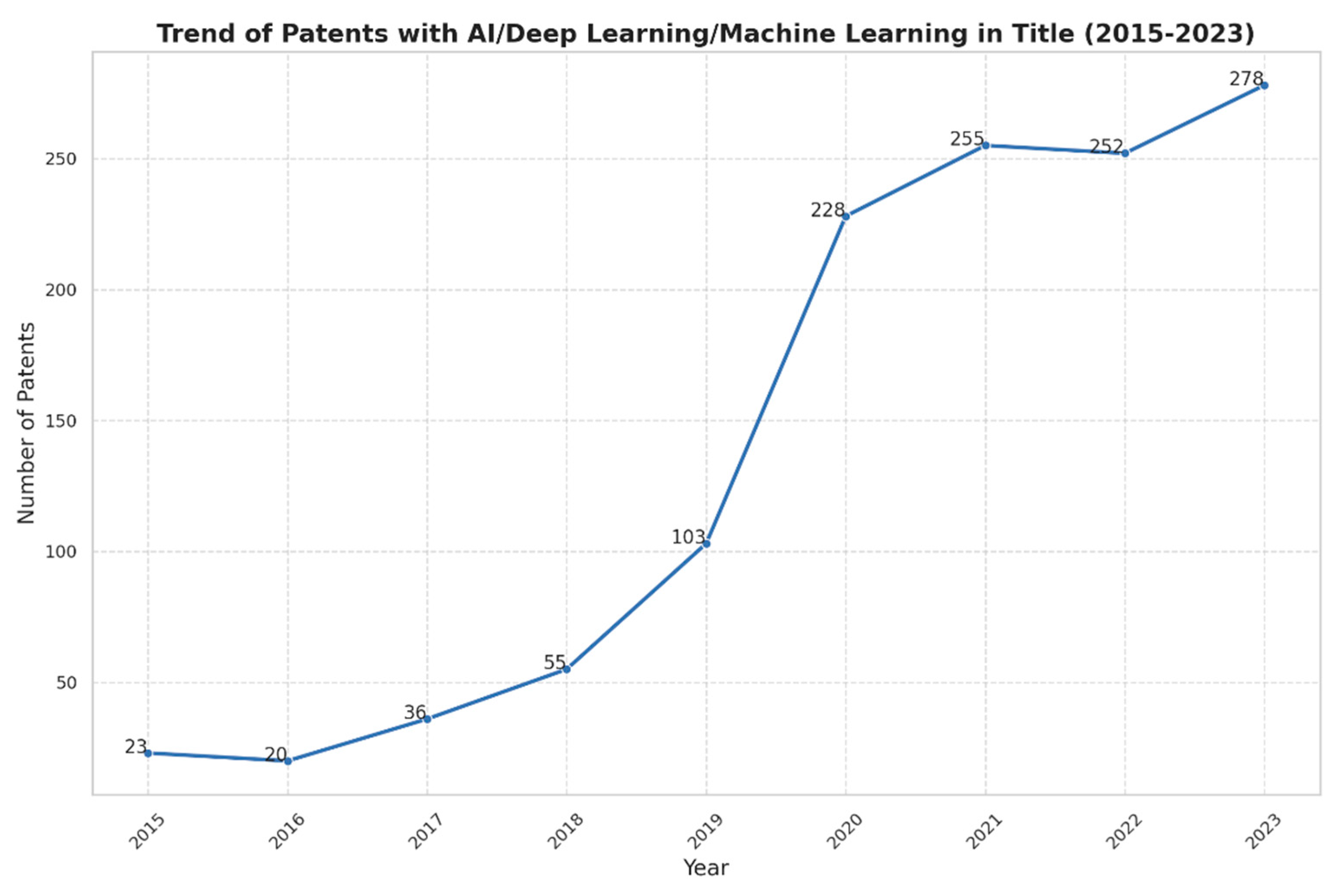
To gain a better knowledge of the usage of deep learning (DL) and machine learning (ML) techniques in remote sensing, we examined patent titles that contained terminology of this kind. As
Figure 1 shows, from 23 in 2015 to 278 in 2023, there was a significant increase in the quantity of these patents, which increased steadily between 2015 and 2023. This tendency suggests that while these technologies will continue to be employed in remote sensing, more advanced deep learning technologies will be necessary to manage more complex and vast remote sensing data and applications [
9].
However, applying deep learning to high-resolution datasets raises major obstacles. The vast number of parameters required for deep neural networks, particularly for high-resolution images, can result in higher processing costs and memory needs, rendering the training process inefficient and potentially infeasible with standard hardware resources. Furthermore, over-parameterization can lead to longer training durations and perhaps overfitting, in which the model memorizes the training data rather than generalizing from it, limiting its usefulness in real-world applications [
10]. To address these difficulties, novel ways for successful training are needed, and while reducing the number of parameters the model should retain its performance. Model pruning and quantization are representative solutions and have been widely used, but each method has its own set of benefits and downsides [
11,
12]. Therefore, in this paper, we introduce a novel network, which is the Kolmogorov-Arnold Network (KAN). The KAN's characteristic could provide a more efficient learning framework [
13]. The main contributions of this paper can be summarized below.
By replacing standard Multi-Layer Perceptrons (MLPs) with KAN, we hope to improve the efficiency and performance of remote sensing applications. Our strategy includes using and comparing different pre-trained Convolutional Neural Networks (CNNs) and Vision Transformer (ViT) models to determine the best KAN pairings, resulting in optimum performance.
Based on the above result, we presented and evaluated our suggested model, KonvNeXt, on four different remote sensing datasets to compare its performance to existing results. This experiment allowed us to scrutinize KonvNeXt's performance in remote sensing fields.
In addition, we applied Explainable AI (XAI) approaches to our model for its interpretability. This process is significant for understanding the decision-making processes of deep learning models, leading to transparency in AI-driven remote sensing applications
2. Related Works
First, we introduce the related research that applied deep learning technologies to the remote sensing datasets. Han and Basalamah showed the effectiveness of a multi-branch system combining pre-trained models for local and global feature extraction in satellite image classification and achieving superior accuracy across three datasets [
14]. By maximizing the performance of small neural networks, Chen et al. used knowledge distillation to increase accuracy on a variety of remote sensing datasets [
15]. Broni-Bediako et al. used automated neural architecture search to develop efficient CNNs for scene classification, which outperformed more traditional models with fewer parameters, such as EuroSAT and BigEarthNet [
16]. Temenos et al. also applied an interpretable deep learning framework to land use classification using SHAP for both high accuracy and enhanced interpretability [
17]. Yadav et al. enhanced classification on the EuroSAT dataset by using pre-trained CNNs and advanced preprocessing techniques, and GoogleNet showed the best performance [
18]. These studies highlight advancements in model accuracy, efficiency, and interpretability for remote sensing image classification.
Then, we introduce the research that utilized KAN for classification or regression. In satellite traffic forecasting, Vaca-Rubio et al. showed that KANs performed better with fewer parameters than traditional MLPs while yielding greater accuracy. The substantial influence of KAN-specific factors was demonstrated by that research, which highlighted their potential for adaptive forecasting models [
19]. Bozorgasl and Chen addressed diverse data distribution across clients by developing Wavelet Kolmogorov-Arnold Networks (Wav-KAN) for hybrid learning. Extensive trials on datasets including MNIST, CIFAR10, and CelebA validated their improvements, which were substantially increased by their incorporation of wavelet-based activation functions [
20]. Using KANs, Abueidda and Pantidis created DeepONets to develop efficient substitutes for mechanics problems. Their approach required fewer learnable parameters than traditional MLP-based models, and it was validated in computational solid mechanics. This demonstrates notable computational speedups and efficiency, making it suitable for high-dimensional and complex engineering applications [
21].
While previous research has utilized pre-trained models, knowledge distillation, NAS, and interpretability frameworks to enhance performance on remote sensing datasets, our technique focuses on determining the possibility of applying KAN to the RS dataset. Our suggested methodology makes sense with the current trends of KAN, which provide a new way for optimization in remote sensing applications. Our integration of KAN with ConvNeXt indicates its capacity to handle remote sensing datasets effectively, unlike other approaches that rely on complex multi-branch frameworks or preprocessing procedures, offering a viable alternative for future study in this sector.
3. Materials and Methods
3.1. Dataset Description and processing
Four different datasets, including EuroSAT, Optimal-31, AID, and Merced were used in this experiment. The EuroSAT dataset proposed by Helber et al. is used to categorize land cover and land use. This collection has 27,000 photographs from 34 different places in Europe, divided into ten categories: annual crop, forest, herbaceous vegetation, highway, industrial, pasture, permanent crop, residential, river, and sea lake [
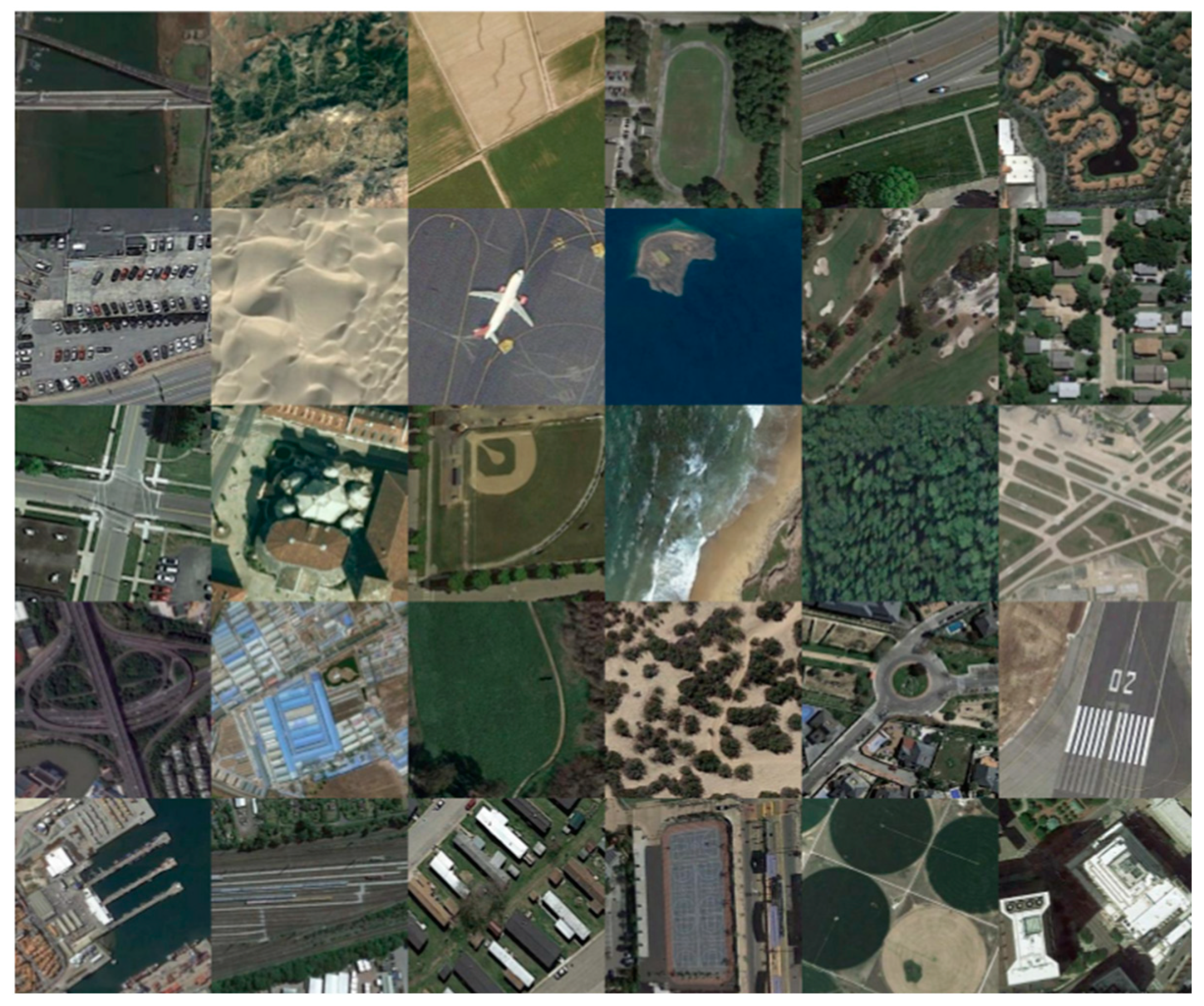
22]. The OPTIMAL-31 dataset consists of 1860 aerial images sourced from Wang et al. This dataset includes 31 different land use types, with each type represented by 60 images of 256×256 pixels, boasting a spatial resolution of 0.3 meters [
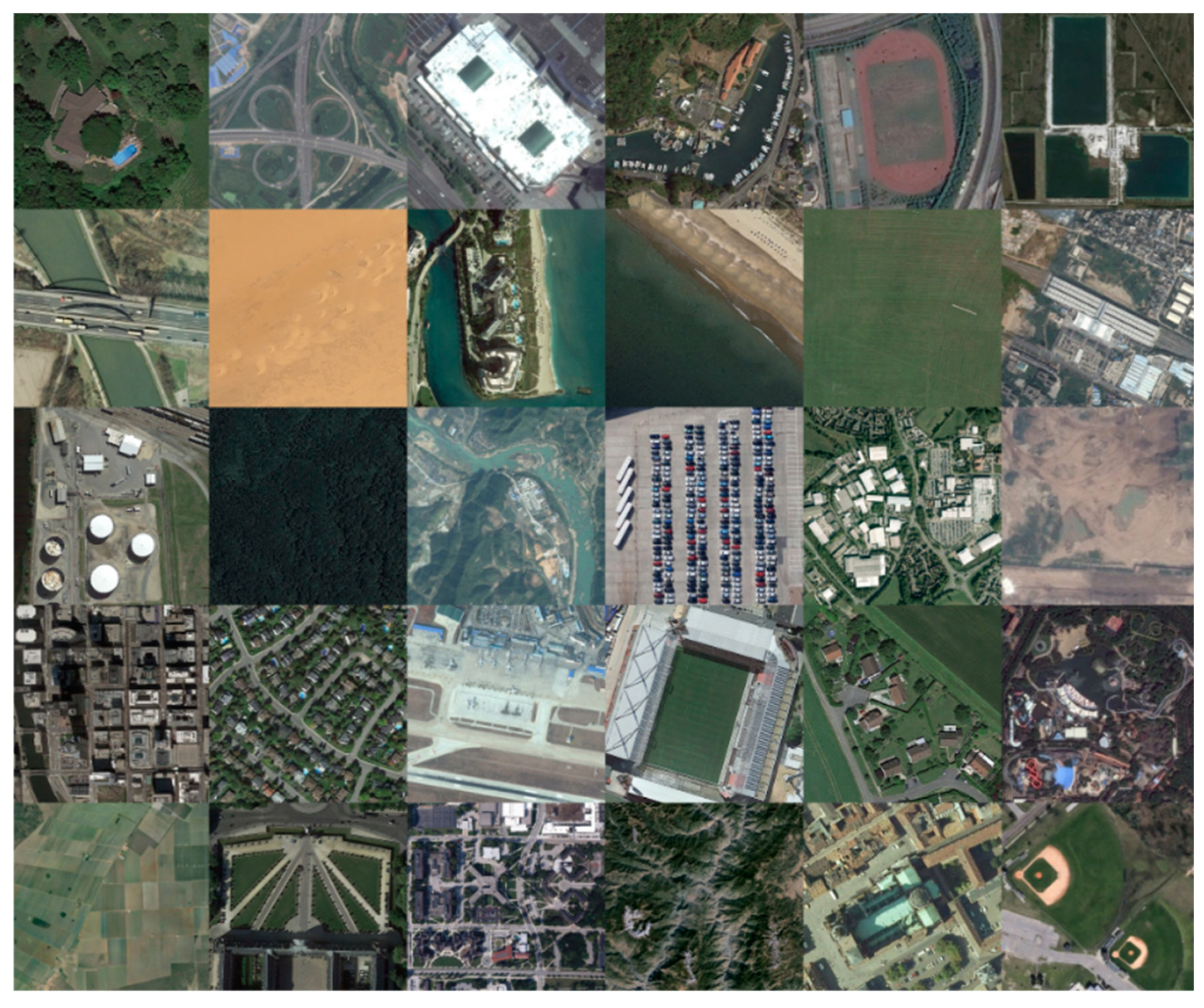
23]. AID is a large-scale aerial image dataset sourced from Google Earth, 600 × 600 pixels, containing 10,000 images across 30 scene types such as airport, forest, and residential areas. Despite post-processing, these images are proven comparable to real optical aerial images for land use and cover mapping [
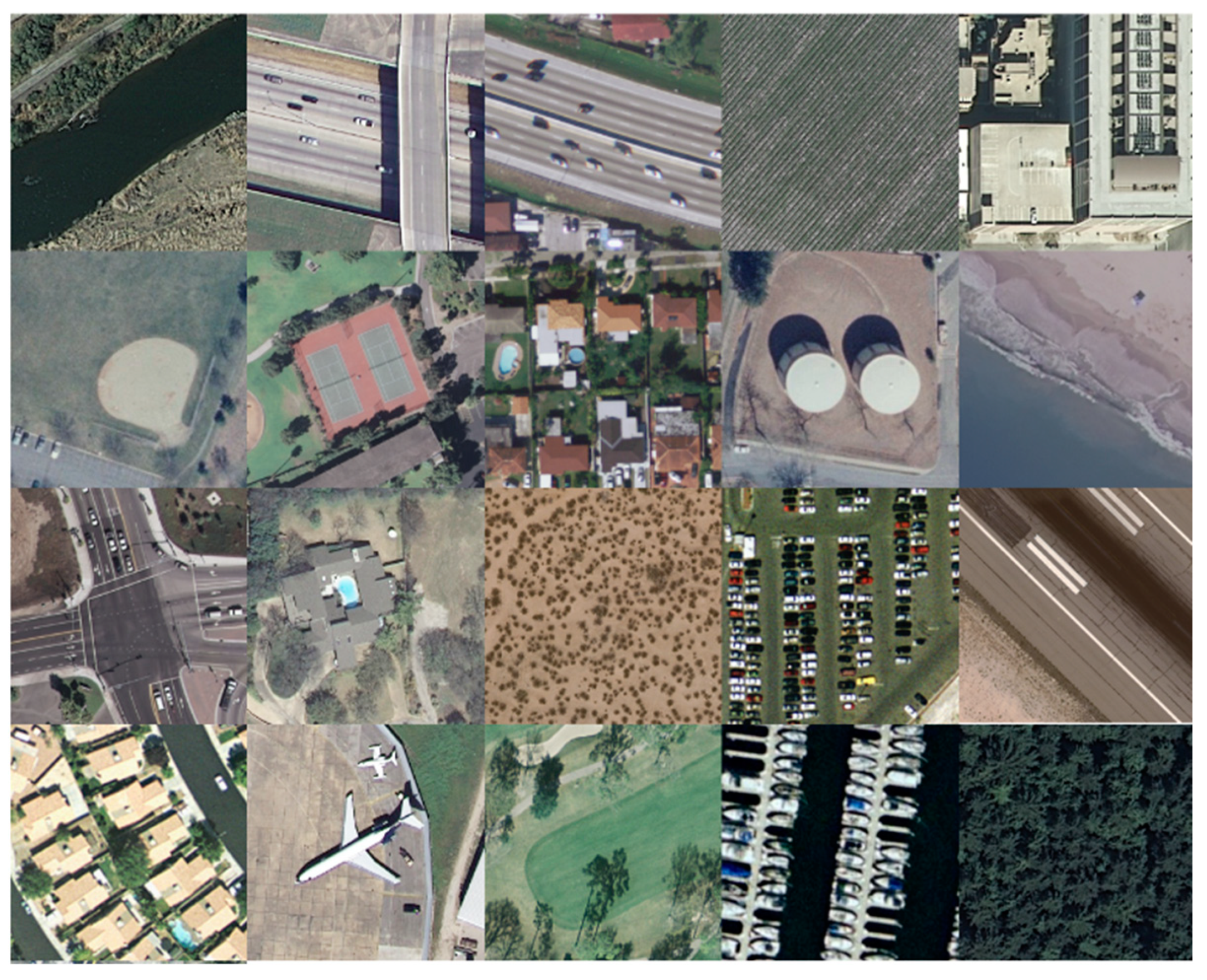
24]. Merced consists of 21 land use classes, with 100 images per class, each measuring 256x256 pixels. The images were manually extracted from the USGS National Map Urban Area Imagery collection, featuring a pixel resolution of 1 foot [
25].
Figure 2,
Figure 3,
Figure 4 and
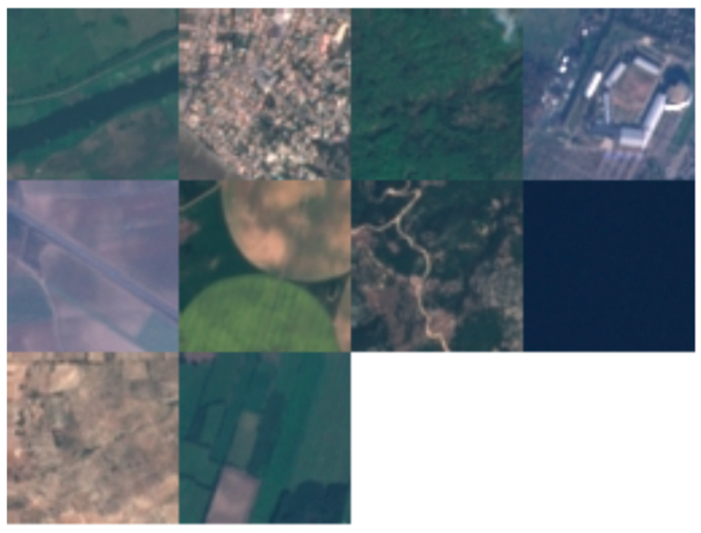
Figure 5 describe examples from each dataset.
The dataset has been divided into three sections for experimentation: approximately 70% of the data is allocated for training, 15% for validation, and 15% for testing. As part of the preparation of the dataset, images are resized to 224 × 224 pixels and normalized using the mean and standard deviation values of ImageNet (mean = [0.485, 0.456, 0.406] and std = [0.229, 0.224, 0.225]). The transformations applied to the data include normalization, conversion to tensors, random horizontal and vertical flips, and random resizing of the cropped images.
3.2. ConvNeXt
Based on conventional ConvNet methods, the ConvNeXt algorithm explicitly modernizes the ResNet model by integrating several Vision Transformers (VIT) design features. As
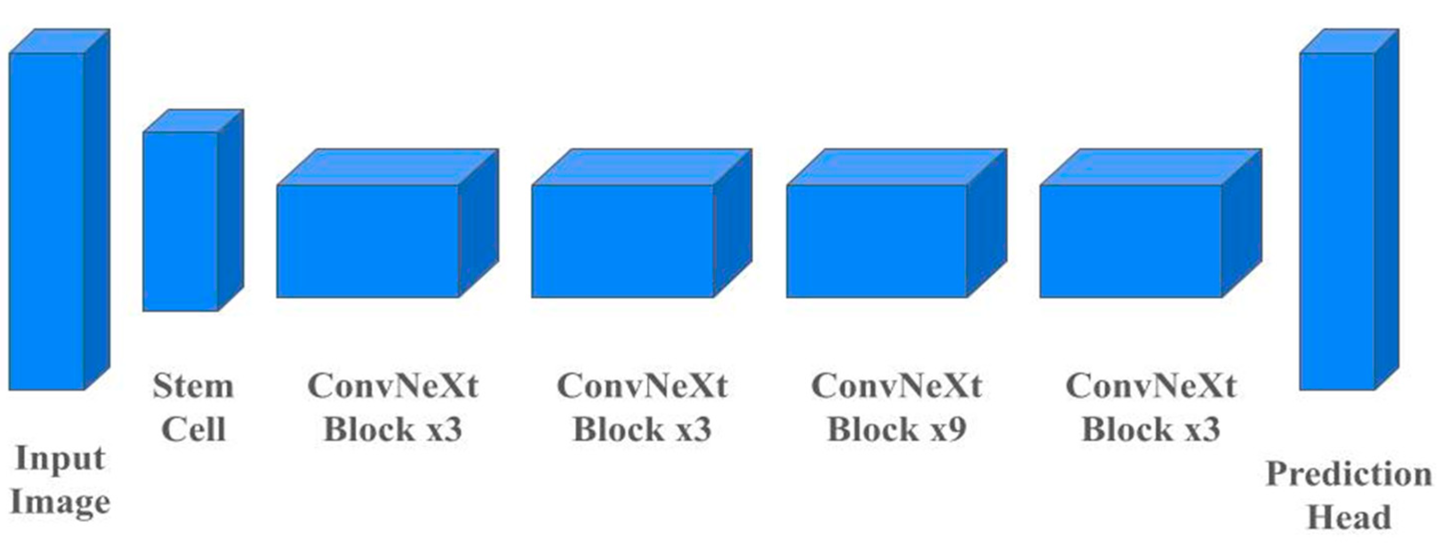
Figure 6 describes, the main structural changes include converting the stem cell to a patchify layer, which divides the input picture into smaller, non-overlapping patches and treats each as a sequence token for additional processing. The algorithm adopts an inverted bottleneck block, used by MobileNetV2, to expand the number of channels before reducing them, capturing spatial and channel-wise features with reduced computational cost. Depthwise convolutions with larger network widths process each input channel separately, which could reduce computational complexity, while pointwise convolutions (1x1 convolution) combine information across channels. Moreover, ConvNeXt applies big kernel sizes for convolutions, Gaussian Error Linear Unit (GELU) activation functions, and LayerNorm which is also the main strategy of the vision transformer. With these modifications, the ConvNeXt could achieve better accuracy than VIT models. Furthermore, by adjusting the hidden dimension sizes, there are several versions such as ConvNeXt-tiny, and ConvNeXt-large [
26,
27].
3.3. Kolmogorov Arnold Network
Inspired by the Kolmogorov-Arnold representation theorem, Kolmogorov-Arnold Networks (KANs) is a sophisticated kind of neural network with learnable activation functions on edges as opposed to fixed activations on nodes in conventional Multi-Layer Perceptrons (MLPs). B-splines, piecewise polynomial functions defined by control points and knots, parameterize these activation functions. Spline-parameterized functions
change each input feature
, aggregate the results into intermediate values for each q, and then pass the values through functions
. The total of these converted values is the final output f(x) which enables the network to effectively and flexibly capture complex data patterns. The activation functions in KANs are a combination of a Basis Function and a Spline, with the Basis Function often being the Sigmoid Linear Unit (SiLU), defined as
. The spline component
uses B-spline basis functions Bi(x) and coefficients ci, which are learned during training and
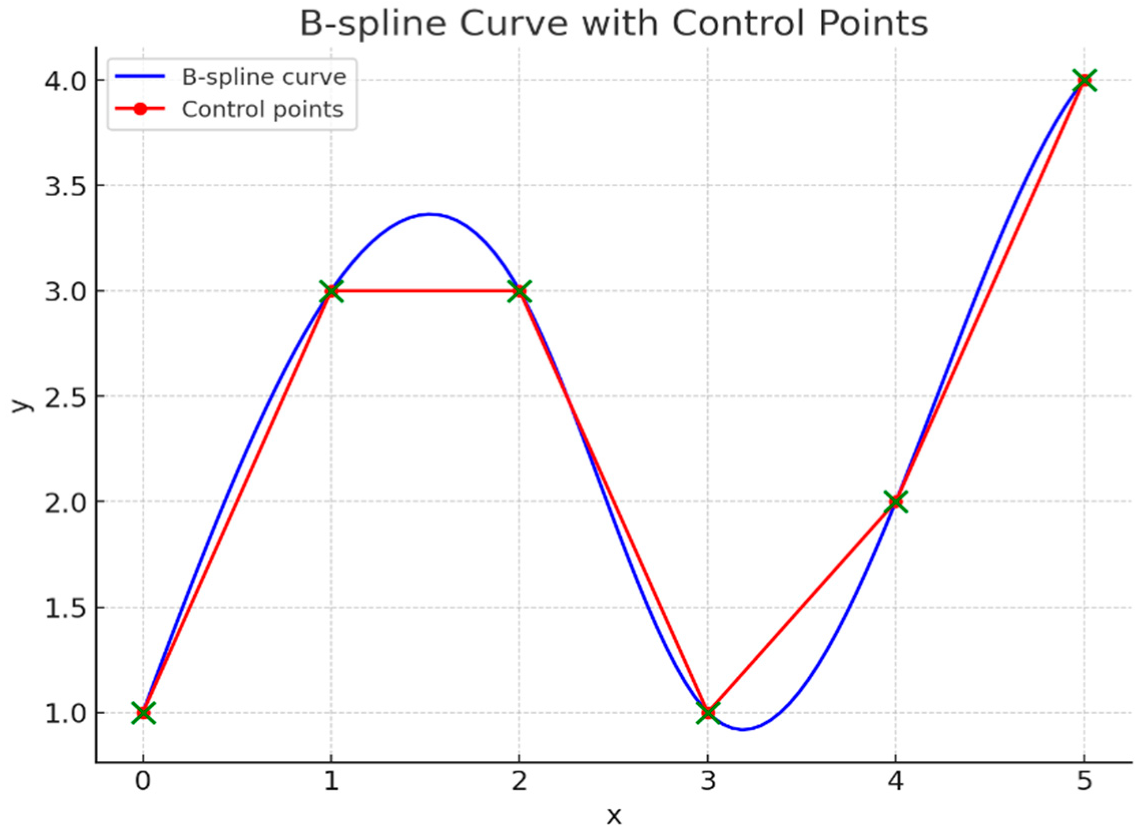
Figure 7 depicts the plot. These coefficients determine the final shape of the activation functions, replacing the need for traditional linear transformation parameters W and b in MLPs.
There are also multiple neurons in the KAN which is similar to that of the MLP. Each hidden layer contains nodes that aggregate the inputs from the previous layer. The output of each node is determined by the spline-parameterized functions of the incoming edges. As data flows through the network, each input to a node is transformed by the B-spline functions on the edges. The transformed inputs are then aggregated (usually by summation) at the node. This aggregation forms the input to the next layer. The training process in KANs involves adjusting the control points and knots of the B-splines to minimize the loss function, and there are three key steps. The first is to compute the output by passing inputs through the network and applying spline transformations at each edge. Backpropagation computes gradients of the loss concerning the control points and knots. These gradients are utilized to update the parameters using optimization algorithms like gradient descent. KANs exhibit various advantages over MLPs, including better accuracy and interpretability with fewer parameters. They achieve this by having smaller architectures that can perform comparably or better than larger MLPs in tasks such as data fitting and partial differential equation (PDE) solving. Since KANs can be depicted, they help discover mathematical and physical laws in scientific applications. Moreover, KANs can aid in preventing catastrophic forgetting, a neural network problem when the learning of new information causes the loss of previously learned information. One notable drawback of KANs over MLPs is their slower training pace, which optimization can address [
13,
28].
The formula for the Kolmogorov-Arnold Network (KAN) is given by:
The function f (x) in a KAN, where
are spline functions and Φq are transformations.
φ(x) denotes the activation function, w is the weight, b(x) is the basis function, and spline(x) is the spline function.
b(x) is the basis function, implemented as silu(x) (Sigmoid Linear Unit).
3.4. ConvNeXt Kolmogorov-Arnold Networks: KonvNeXt
The proposed approach combines KAN and the ConvNeXt architecture to improve a pre-trained ConvNeXt model's learning capacity. To enhance feature-extracting performance, we adopted the models that were trained with the Imagenet datasets. The model adds two KANLinear layers instead of the conventional MLP classifier. Unlike typical neural networks, which use fixed activation functions on the nodes, KANLinear layers use learnable activation functions on the edges. More stability and flexibility are provided by the use of B-splines to describe these activation functions. By substituting these spline functions for linear weights in the KANLinear layer, the model is better able to execute the model efficiently because the KAN layer does not consume much memory compared to the original layers. This approach is not only applicable to ConvNeXt, which means it could replace neural net layers in various deep learning models.
4. Results
First, we applied various CNN-based models that were pre-trained on the ImageNet dataset to figure out the most optimal one on the EuroSAT dataset. Typically, these pre-trained networks utilize MLP layers for classification or regression tasks. However, since our research aimed to demonstrate the potential of replacing MLP with KAN, we substituted the MLP with KAN in these models. We evaluated several models, including VGG16, MobileNetV2, EfficientNet, ConvNeXt, ResNet101, and ViT [
29,
30,
31,
26,
32,
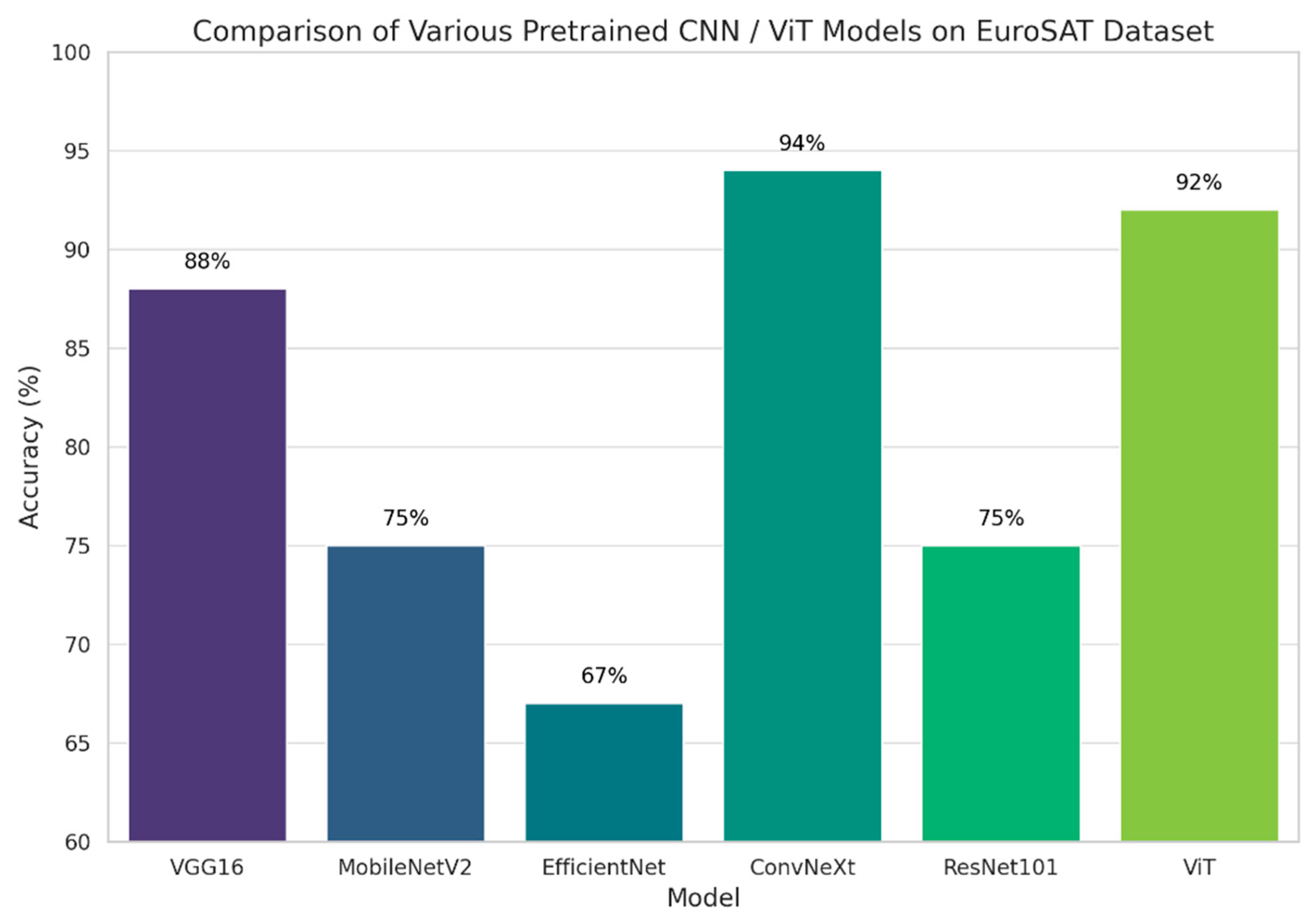
33]. The observed accuracies for these models were 88%, 75%, 67%, 94%, 75%, and 92%, respectively, as shown in
Figure 8. To demonstrate the efficiency of KAN, we initially configured each KAN layer with 256 nodes and subsequently reduced the nodes to 32 for comparison. The results revealed identical performance between both configurations. Both setups achieved an accuracy of 94% in the first epoch, which increased to 96% in the second epoch, maintaining this accuracy in the subsequent epochs. This experiment indicates that KAN layers can achieve high accuracy with fewer training epochs, even when the number of nodes is significantly reduced and this proved the efficiency of the KAN layer. From the proposed approach of integrating ConvNeXt with KAN, we figured out interesting results in terms of classification accuracy per epoch. The model achieved an accuracy of 94% in the first epoch, which increased to 96% in the second epoch. This accuracy of 96% was maintained consistently through the fifth epoch. These results suggest that even with one or two epochs, sufficient training of KAN-based networks can be achieved. Despite the drawback that KAN is ten times slower than traditional MLPs, the reduced number of necessary training epochs effectively overcomes this downside [
34].
Then, with our KonvNeXt model, we tested three more popular datasets in remote sensing fields, including Optimal-31, AID, and Merced. We chose these datasets since there already exists a paper that utilized VIT for remote sensing datasets [
35]. As
Table 1 describes, with 25 epochs, our proposed model achieved 90.59% for Optimal-31, 94.1% for AID, and 98.1% for Merced. Since Bazi et al.’s VIT model yielded 92.76% for Optimal-31, 91.76% for AID, and 92.76% for Merced datasets, this result implied that our proposed approach resulted in better performance than the VIT models. This result is meaningful since the proposed model did not demand long training time. For instance, it took 107.14 seconds for the Optimal-31 dataset, 545.91 seconds for the AID dataset, and Merced for 107.63 seconds. Since Bazi et al.’s model took an average of 30 minutes to train those datasets, these results proved that our approach not only achieved high performance but also a fast speed which could overcome the original downsides of the KAN models [
35].
In another experiment, we compared the performance of our proposed model to that of the original ConvNeXt models. The ConvNeXt achieved accuracy rates of 84.68%, 94.6%, and 97.8% on the three datasets as depicted in
Table 2. These results indicate that substituting the neural network's linear layers with the KAN layers can be effective in terms of performance and memory efficiency. Interestingly, by using only two layers for comparison, the speed gap between the models was small. This result suggests that the ConvNeXt model with the KAN layer is efficient enough for these remote sensing datasets, even with fewer linear layers.
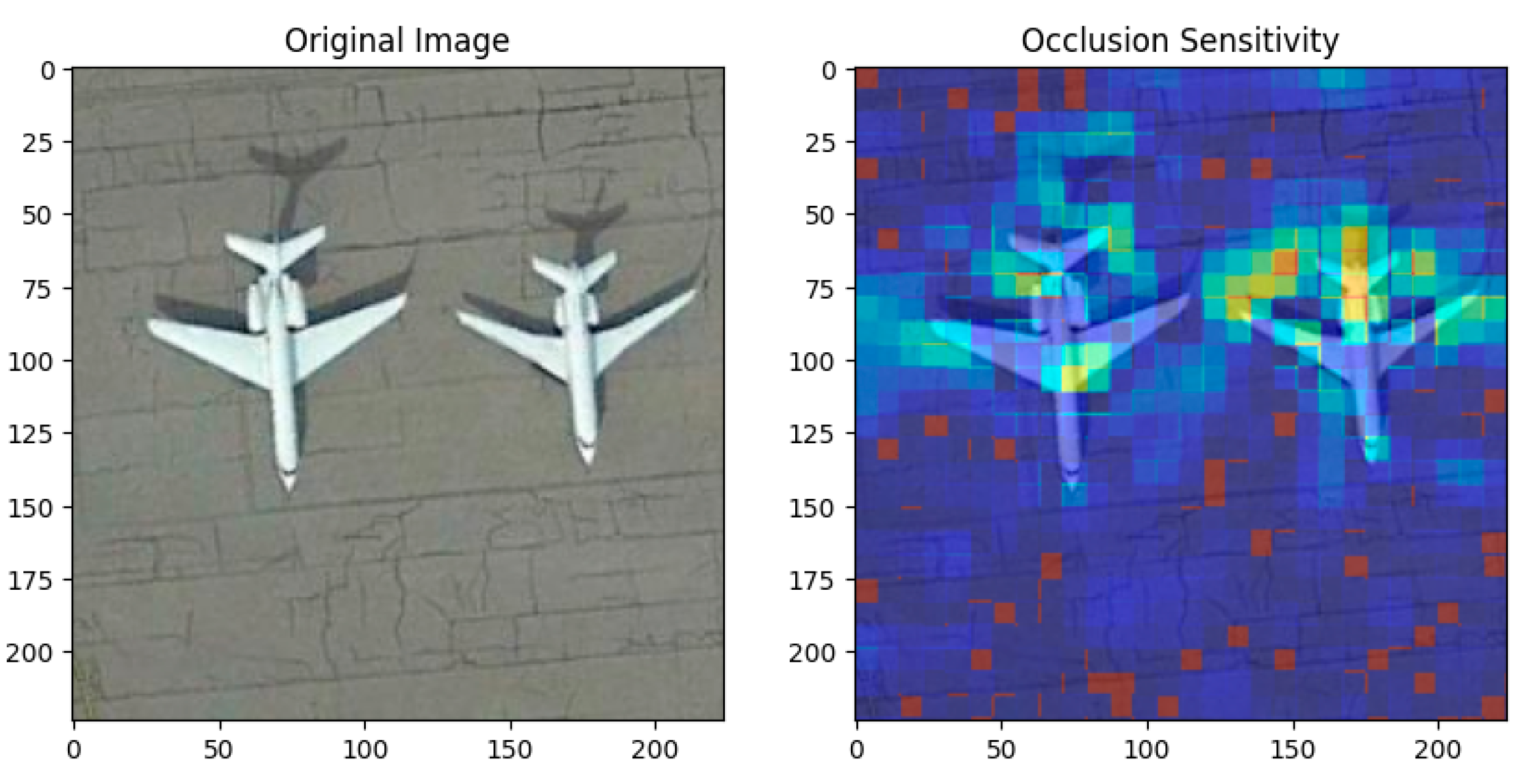
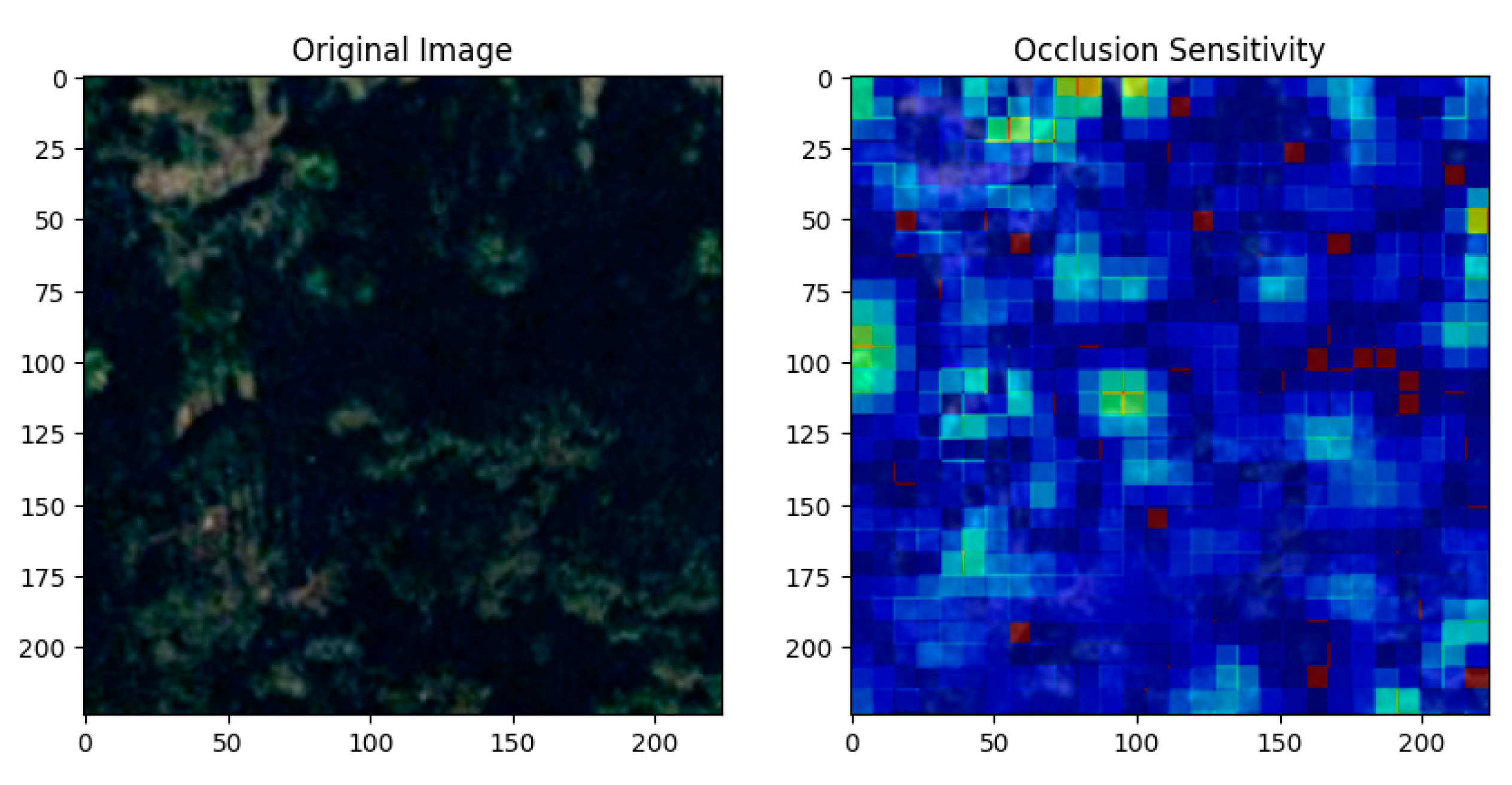
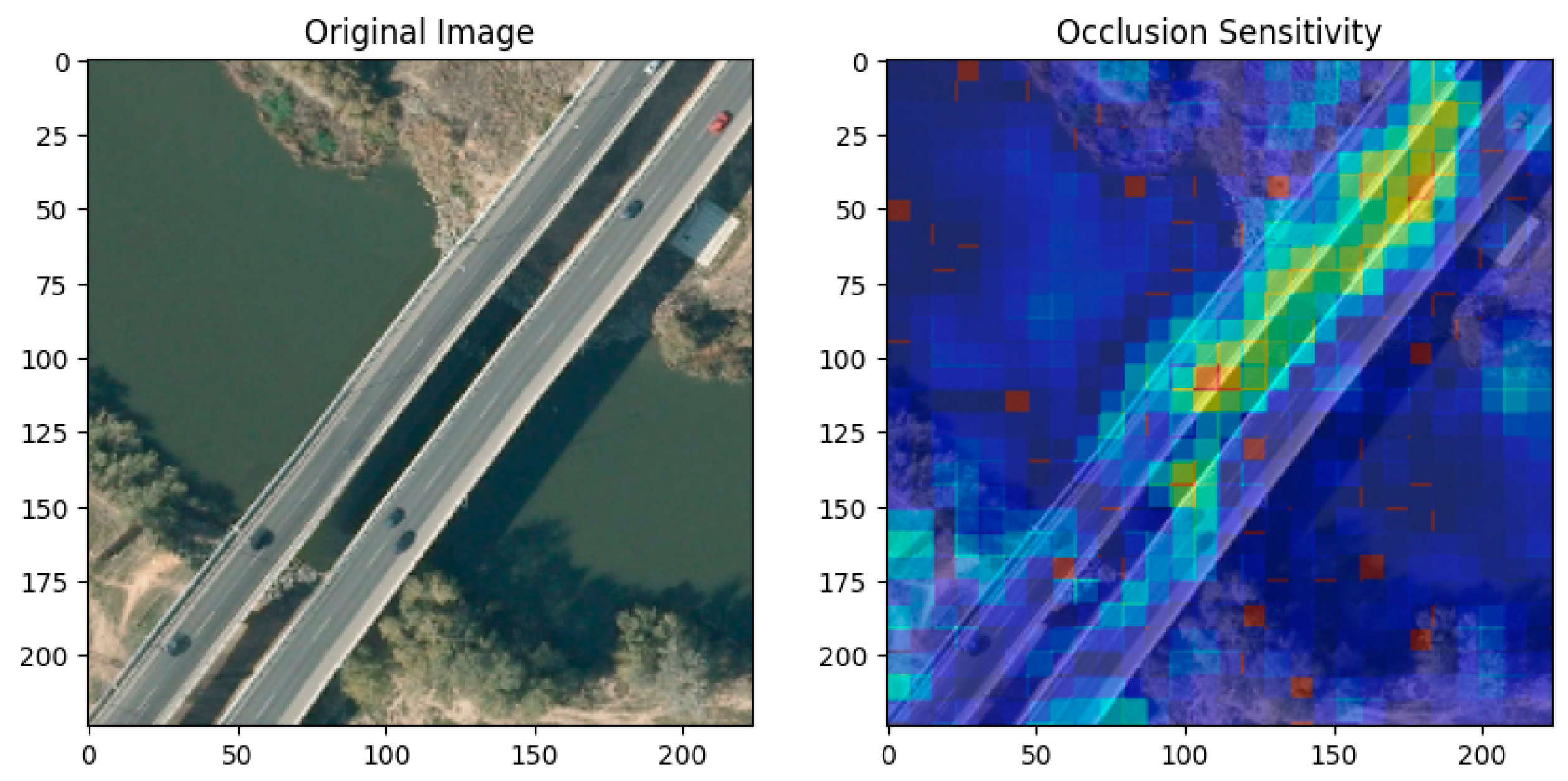
Since our proposed approach utilizes ConvNeXt to capture features from images, XAI methods can be applied to our model. For instance, we applied Occlusion Sensitivity in the above experiments. Occlusion sensitivity is a technique used in explainable AI to identify which regions of an image most influence a model's predictions by systematically occluding parts of the image and observing changes in the output. The heatmap overlay in the right image highlights these influential regions, with red/yellow areas indicating high sensitivity and blue areas indicating low sensitivity, and each results are shown in
Figure 9,
Figure 10 and
Figure 11. The results demonstrated that the proposed model classified the target with reasonable decision-making. Furthermore, this result also shows the potential for applying this model to diverse datasets, where interpreting deep learning is crucial, such as in weather prediction or medical diagnosis [
36].
5. Discussion
This paper introduces the application of Kernel Attention Networks (KAN) to remote sensing datasets by integrating them with the ConvNeXt algorithm. Given that KAN is in its early stages of development and has primarily been tested on MNIST, CIFAR-10, CIFAR-100, and ImageNet datasets, its suitability for specific tasks was previously uncertain. Therefore our work is pioneering in this field, since we evaluated the efficacy of our proposed model, KonvNeXt, by testing it on four different representative remote sensing classification datasets. The experiments demonstrated that KonvNeXt has significant potential for application across various datasets. Additionally, our approach may offer more applicability because many existing deep learning models utilize neural network layers that demand substantial GPU memory based on their parameters. In this context, the KAN layer could serve as a substitute, extending beyond computer vision tasks to include natural language processing (NLP) tasks, even in large language model (LLM) tasks. For future work, we will explore models that consist solely of KAN layers, following the current trend, without merging them with any CNN models, and apply them to remote sensing datasets to compare the performance of KAN to the existing CNN models [
37,
38].
5. Conclusions
The objective of this paper is to introduce the KAN model to the field of remote sensing. To validate the applicability of that model, we conducted several experiments. First, with the EuroSAT dataset, we combined the KAN layer with multiple pretrained CNN models to discover the best fit. We found that ConvNeXt with KAN reached the optimal performance, so we named it the KonvNeXt. For broader validation of the model in the remote sensing fields, the model was tested on three different datasets—Optimal-31, AID, and Merced—and it achieved high performance on both accuracy and speed. Specifically, the model achieved an accuracy of 90.59% on the Optimal-31 dataset, 94.1% on the AID dataset, and 98.1% on the Merced dataset. In terms of processing speed, the model exhibited notable efficiency. For the speed, It processed the Optimal-31 and Merced datasets in 107.63 seconds each, demonstrating a consistent performance. However, the AID dataset, being more complex and larger in scale, took 545.91 seconds to process. These experiments proved that the KonvNeXt could be suitably applied to the remote sensing classification tasks. Furthermore, by utilizing Occlusion Sensitivity, we also demonstrated that the various existing XAI methods could apply to the KonvNeXt, which provided a possibility of its versatilities in various fields, such as medical fields or weather forecasting [
39,
40,
41]. In conclusion, this paper is meaningful as it represents the first approach to applying KAN in remote sensing classification and shows a possibility.
Author Contributions
Conceptualization, C.M.; Methodology, M.C.; Visualization, M.C.; Supervision, C.M.; Project administration, C.M.; Funding acquisition, C.M. All authors have read and agreed to the published version of the manuscript.
Funding
This work was supported by the Ministry of Education of the Republic of Korea and the National Research Foundation of Korea (NRF-2023S1A5A8078960)
Data Availability Statement
Acknowledgments
We would like to express our gratitude to the providers of the datasets used in this study. Our sincere thanks go to Jonathan Roberts for making the Optimal-31 dataset available via Hugging Face, Patrick Helber and contributors for providing the EuroSAT dataset on GitHub, the UC Merced team for making the Merced dataset accessible, and the Captain WHU team for their work on the AID dataset. Their contributions help the advancement of our research.
Conflicts of Interest
The authors declare no conflicts of interest.
References
- Yang, C. High Resolution Satellite Imaging Sensors for Precision Agriculture. Frontiers of Agricultural Science and Engineering 2018. [CrossRef]
- Ma, Y.; Wu, H.; Wang, L.; Huang, B.; Ranjan, R.; Zomaya, A.; Jie, W. Remote Sensing Big Data Computing: Challenges and Opportunities. Future Generation Computer Systems 2015, 51, 47–60. [Google Scholar] [CrossRef]
- Xu, H.; Wang, Y.; Guan, H.; Shi, T.; Hu, X. Detecting Ecological Changes with a Remote Sensing Based Ecological Index (RSEI) Produced Time Series and Change Vector Analysis. Remote Sensing 2019, 11, 2345. [Google Scholar] [CrossRef]
- Milesi, C.; Churkina, G. Measuring and Monitoring Urban Impacts on Climate Change from Space. Remote Sensing 2020, 12, 3494. [Google Scholar] [CrossRef]
- Ustin, S.L.; Middleton, E.M. Current and Near-Term Advances in Earth Observation for Ecological Applications. Ecological Processes 2021, 10. [Google Scholar] [CrossRef] [PubMed]
- Leblois, A.; Damette, O.; Wolfersberger, J. What Has Driven Deforestation in Developing Countries Since the 2000s? Evidence from New Remote-Sensing Data. World Development 2017, 92, 82–102. [Google Scholar] [CrossRef]
- Shafique, A.; Cao, G.; Khan, Z.; Asad, M.; Aslam, M. Deep Learning-Based Change Detection in Remote Sensing Images: A Review. Remote Sensing 2022, 14, 871. [Google Scholar] [CrossRef]
- Adegun, A.A.; Viriri, S.; Tapamo, J.-R. Review of Deep Learning Methods for Remote Sensing Satellite Images Classification: Experimental Survey and Comparative Analysis. Journal of Big Data 2023, 10. [Google Scholar] [CrossRef]
- Google Patents Available online: https://patents.google.com/.
- Liu, S.; Yin, L.; Mocanu, D.C.; Pechenizkiy, M. Do We Actually Need Dense Over-Parameterization? In-Time Over-Parameterization in Sparse Training. Arxiv 2021. [CrossRef]
- Hoefler, T.; Alistarh, D.; Ben-Nun, T.; Dryden, N.; Peste, A. Sparsity in Deep Learning: Pruning and Growth for Efficient Inference and Training in Neural Networks. Journal of Machine Learning Research 2021, 22, 1–124. [Google Scholar]
- Vadera, S.; Ameen, S. Methods for Pruning Deep Neural Networks. IEEE Access 2022, 10, 63280–63300. [Google Scholar] [CrossRef]
- Liu, Z.; Wang, Y.; Vaidya, S.; Ruehle, F.; Halverson, J.; Soljačić, M.; Hou, T.Y.; Tegmark, M. KAN: Kolmogorov-Arnold Networks. arXiv 2024. [CrossRef]
- Khan, S.D.; Basalamah, S. Multi-Branch Deep Learning Framework for Land Scene Classification in Satellite Imagery. Remote Sensing 2023, 15, 3408. [Google Scholar] [CrossRef]
- Chen, G.; Zhang, X.; Tan, X.; Cheng, Y.; Dai, F.; Zhu, K.; Gong, Y.; Wang, Q. Training Small Networks for Scene Classification of Remote Sensing Images via Knowledge Distillation. Remote Sensing 2018, 10, 719. [Google Scholar] [CrossRef]
- Broni-Bediako, C.; Murata, Y.; Mormille, L.H.B.; Atsumi, M. Searching for CNN Architectures for Remote Sensing Scene Classification. IEEE Transactions on Geoscience and Remote Sensing 2022, 60, 1–13. [Google Scholar] [CrossRef]
- Temenos, A.; Temenos, N.; Kaselimi, M.; Doulamis, A.; Doulamis, N. Interpretable Deep Learning Framework for Land Use and Land Cover Classification in Remote Sensing Using SHAP. IEEE Geoscience and Remote Sensing Letters 2023, 20, 1–5. [Google Scholar] [CrossRef]
- Yadav, D.; Kapoor, K.; Yadav, A.K.; Kumar, M.; Jain, A.; Morato, J. Satellite Image Classification Using Deep Learning Approach. Earth Science Informatics 2024, 17, 2495–2508. [Google Scholar] [CrossRef]
- Vaca-Rubio, C.J.; Blanco, L.; Pereira, R.; Caus, M. Kolmogorov-Arnold Networks (KANs) for Time Series Analysis. arXiv 2024. [CrossRef]
- Bozorgasl, Z.; Chen, H. WAV-KAN: Wavelet Kolmogorov-Arnold Networks. Social Science Research Network 2024. [CrossRef]
- Abueidda, D.W.; Pantidis, P.; Mobasher, M.E. DeepOKAN: Deep Operator Network Based on Kolmogorov Arnold Networks for Mechanics Problems. arXiv 2024. [CrossRef]
- Helber, P.; Bischke, B.; Dengel, A.; Borth, D. EuroSAT: A Novel Dataset and Deep Learning Benchmark for Land Use and Land Cover Classification. arXiv 2017. [CrossRef]
- Wang, Q.; Liu, S.; Chanussot, J.; Li, X. Scene Classification with Recurrent Attention of VHR Remote Sensing Images. IEEE Transactions on Geoscience and Remote Sensing 2019, 57, 1155–1167. [Google Scholar] [CrossRef]
- Xia, G.-S.; Hu, J.; Hu, F.; Shi, B.; Bai, X.; Zhong, Y.; Zhang, L.; Lu, X. AID: A Benchmark Data Set for Performance Evaluation of Aerial Scene Classification. IEEE Transactions on Geoscience and Remote Sensing 2017, 55, 3965–3981. [Google Scholar] [CrossRef]
- Yang, Y.; Newsam, S. Bag-of-Visual-Words and Spatial Extensions for Land-Use Classification. 2010. [Google Scholar]
- Liu, Z.; Mao, H.; Wu, C.-Y.; Feichtenhofer, C.; Darrell, T.; Xie, S. A ConvNet for the 2020s. arXiv 2022. [CrossRef]
- Cheon, M.; Choi, Y.-H.; Kang, S.-Y.; Choi, Y.; Lee, J.-G.; Kang, D. KARINA: An Efficient Deep Learning Model for Global Weather Forecast. arXiv 2024. [CrossRef]
- Schmidt-Hieber, J. The Kolmogorov–Arnold Representation Theorem Revisited. Neural Networks 2021, 137, 119–126. [Google Scholar] [CrossRef]
- Simonyan, K.; Zisserman, A. Very Deep Convolutional Networks for Large-Scale Image Recognition. Computer Vision and Pattern Recognition 2014.
- Sandler, M.; Howard, A.; Zhu, M.; Zhmoginov, A.; Chen, L.-C. MobileNetV2: Inverted Residuals and Linear Bottlenecks. Arxiv 2018. [CrossRef]
- Tan, M.; Le, Q., V. EfficientNet: Rethinking Model Scaling for Convolutional Neural Networks. arXiv 2019. [CrossRef]
- He, K.; Zhang, X.; Ren, S.; Sun, J. Deep Residual Learning for Image Recognition. 2016. [Google Scholar]
- Dosovitskiy, A.; Beyer, L.; Kolesnikov, A.; Weissenborn, D.; Zhai, X.; Unterthiner, T.; Dehghani, M.; Minderer, M.; Heigold, G.; Gelly, S.; et al. An Image Is Worth 16x16 Words: Transformers for Image Recognition at Scale. International Conference on Learning Representations 2021.
- Cheon, M. Kolmogorov-Arnold Network for Satellite Image Classification in Remote Sensing. arXiv 2024. [CrossRef]
- Bazi, Y.; Bashmal, L.; Rahhal, M.M.A.; Dayil, R.A.; Ajlan, N.A. Vision Transformers for Remote Sensing Image Classification. Remote Sensing 2021, 13, 516. [Google Scholar] [CrossRef]
- Zeiler, M.D.; Fergus, R. Visualizing and Understanding Convolutional Networks. arXiv 2013. [CrossRef]
- Cheon, M. Demonstrating the Efficacy of Kolmogorov-Arnold Networks in Vision Tasks. arXiv 2024. [CrossRef]
- Drokin, I. Kolmogorov-Arnold Convolutions: Design Principles and Empirical Studies. arXiv 2024. [CrossRef]
- Ham, Y.-G.; Kim, J.-H.; Luo, J.-J. Deep Learning for Multi-Year ENSO Forecasts. Nature 2019, 573, 568–572. [Google Scholar] [CrossRef] [PubMed]
- Mun, C.; Ha, H.; Lee, O.; Cheon, M. Enhancing AI-CDSS with U-AnoGAN: Tackling Data Imbalance. Computer Methods and Programs in Biomedicine 2024, 244, 107954. [Google Scholar] [CrossRef]
- Cheon, M. SR-ANoGAN: You Never Detect Alone. Super Resolution in Anomaly Detection (Student Abstract). Proceedings of the AAAI Conference on Artificial Intelligence 2023, 37, 16194–16195. [Google Scholar] [CrossRef]
Figure 1.
Annual Trends in AI/Deep Learning/Machine Learning Patents (2015-2023).
Figure 1.
Annual Trends in AI/Deep Learning/Machine Learning Patents (2015-2023).
Figure 2.
Example images of AID datasets used in the experiment.
Figure 2.
Example images of AID datasets used in the experiment.
Figure 3.
Example images of Optimal-31 datasets used in the experiment.
Figure 3.
Example images of Optimal-31 datasets used in the experiment.
Figure 4.
Example images of Merced datasets used in the experiment.
Figure 4.
Example images of Merced datasets used in the experiment.
Figure 5.
Example images of EuroSAT datasets used in the experiment.
Figure 5.
Example images of EuroSAT datasets used in the experiment.
Figure 6.
An overall architecture of the ConvNeXt model was used as the backbone model in the experiment. It begins with an input image, followed by a stem cell, and then sequentially passes through multiple ConvNeXt blocks (with repetitions as indicated: 3, 3, 9, 3). The final stage is the prediction head, which outputs the model's predictions.
Figure 7.
An example of a B-spline Curve with Control Points which shows a B-spline curve (blue) with its control points (red) and connecting lines.
Figure 7.
An example of a B-spline Curve with Control Points which shows a B-spline curve (blue) with its control points (red) and connecting lines.
Figure 8.
: Comparison of Various pretrained CNN / ViT Models on the EuroSAT Dataset.
Figure 8.
: Comparison of Various pretrained CNN / ViT Models on the EuroSAT Dataset.
Figure 9.
: Occlusion Sensitivity Example When using the Optimal-31 dataset with the KonvNeXt model: The original aerial view of an aircraft that served as the KonvNeXt model's input is seen in the left picture.
Figure 9.
: Occlusion Sensitivity Example When using the Optimal-31 dataset with the KonvNeXt model: The original aerial view of an aircraft that served as the KonvNeXt model's input is seen in the left picture.
Figure 10.
: An Illustration of Occlusion Sensitivity When using the Merced dataset with the KonvNeXt model: The original aerial photograph of a forest that served as the KonvNeXt model's input is seen in the left picture.
Figure 10.
: An Illustration of Occlusion Sensitivity When using the Merced dataset with the KonvNeXt model: The original aerial photograph of a forest that served as the KonvNeXt model's input is seen in the left picture.
Figure 11.
Example of Occlusion Sensitivity Applied to the KonvNeXt model with AID dataset: The left image shows the original aerial view of a bridge used as input for the KonvNeXt model.
Figure 11.
Example of Occlusion Sensitivity Applied to the KonvNeXt model with AID dataset: The left image shows the original aerial view of a bridge used as input for the KonvNeXt model.
Table 1.
Summary of accuracy and speed when applying KonvNeXt on three different datasets: Optimal-31, AID, and Merced.
Table 1.
Summary of accuracy and speed when applying KonvNeXt on three different datasets: Optimal-31, AID, and Merced.
| accuracy/speed |
Optimal-31 |
AID |
Merced |
| accuracy |
90.59% |
94.1% |
98.1% |
| speed |
107.63 sec |
545.91 sec |
107.63 sec |
Table 2.
Summary of accuracy and speed when applying ConvNeXt on three different datasets: Optimal-31, AID, and Merced.
Table 2.
Summary of accuracy and speed when applying ConvNeXt on three different datasets: Optimal-31, AID, and Merced.
| accuracy/speed |
Optimal-31 |
AID |
Merced |
| accuracy |
84.68% |
94.6% |
97.8% |
| speed |
106.63 sec |
549.3 sec |
106.64 sec |
|
Disclaimer/Publisher’s Note: The statements, opinions and data contained in all publications are solely those of the individual author(s) and contributor(s) and not of MDPI and/or the editor(s). MDPI and/or the editor(s) disclaim responsibility for any injury to people or property resulting from any ideas, methods, instructions or products referred to in the content. |
© 2024 by the authors. Licensee MDPI, Basel, Switzerland. This article is an open access article distributed under the terms and conditions of the Creative Commons Attribution (CC BY) license (https://creativecommons.org/licenses/by/4.0/).
