Submitted:
08 July 2024
Posted:
09 July 2024
You are already at the latest version
Abstract
Keywords:
1. Introduction
2. Literature Review
2.1. Weather and Milk Productivity
2.2. Econometric Analysis of Climate Effects on Agricultural Production
3. Materials and Methods
3.1. Model Specification
3.2. Data
4. Results
4.1. Results without Spatial Interactions
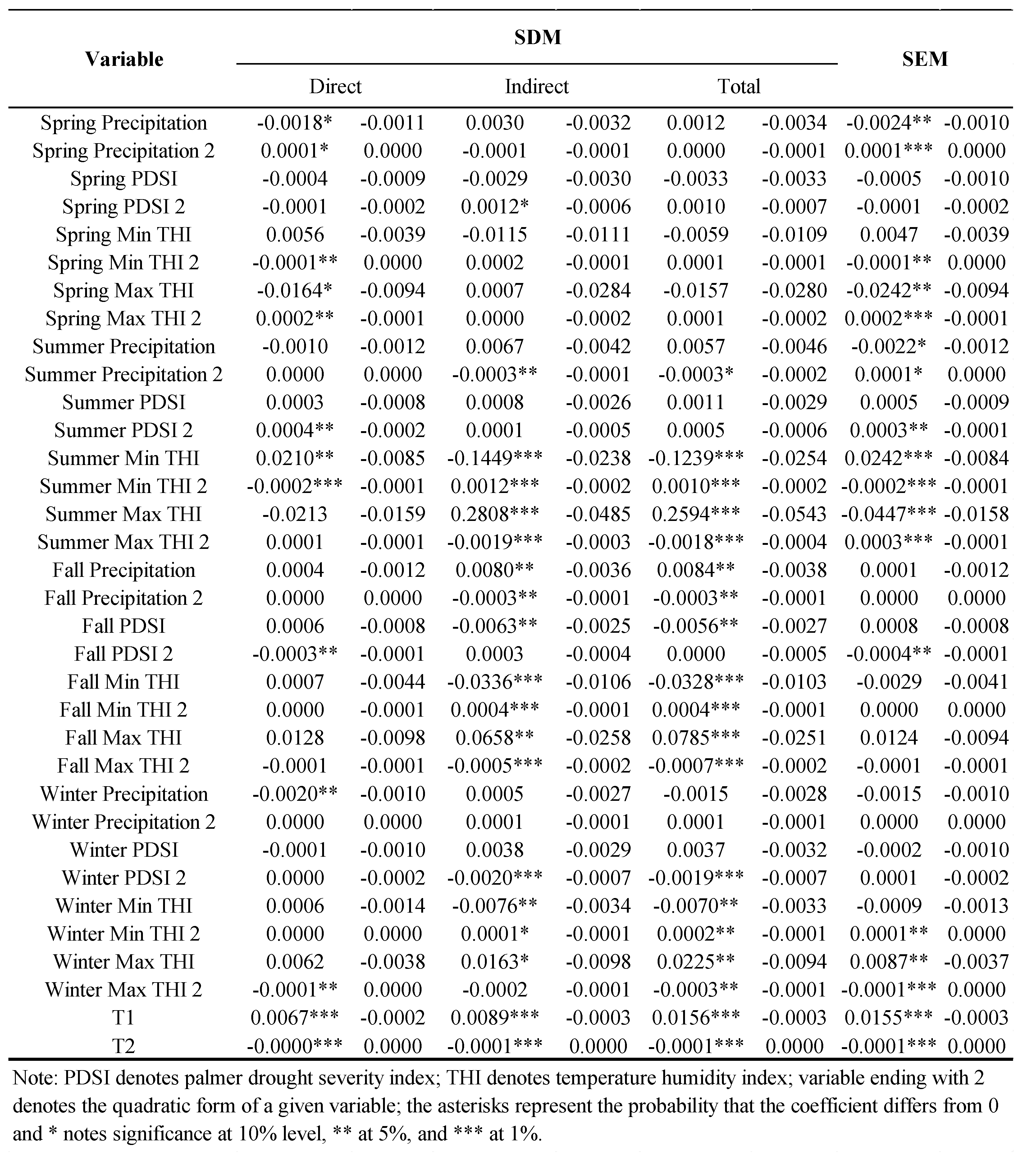
4.2. Spatial Panel Model Results
4.3. Model Comparison
5. Conclusions and Discussion
Author Contributions
Funding
Data Availability Statement
Conflicts of Interest
| 1 | Please refer to https://quickstats.nass.usda.gov/
|
References
- IPCC. Climate Change 2022: Impacts, Adaptation, and Vulnerability. Contribution of Working Group II to the Sixth Assessment Report of the Intergovernmental Panel on Climate Change (H.-O. Pörtner, D.C. Roberts, M. Tignor, E.S. Poloczanska, K. Mintenbeck, A. Alegría, M. Craig, S. Langsdorf, S. Löschke, V. Möller, A. Okem, B. Rama, Eds.). Cambridge University Press. Cambridge University Press, Cambridge, UK and New York, NY, USA, 2022, 3056 pp.. [CrossRef]
- Hristov, A.N.; Degaetano, A.T.; Rotz, C.A.; Hoberg, E.; Skinner, R.; Felix, T.; Li, H.; Patterson, P.H.; Roth, G.; Hall, M.; et al. Climate Change Effects on Livestock in the Northeast US and Strategies for Adaptation. Clim. Change 2018, 146, 33–45. [CrossRef]
- Thornton, P.K.; Van de Steeg, J.; Notenbaert, A.; Herrero, M. The Impacts of Climate Change on Livestock and Livestock Systems in Developing Countries: A Review of What We Know and What We Need to Know. Agric. Syst. 2009, 101, 113–127. [CrossRef]
- Mauger, G.; Bauman, Y.; Nennich, T.; Salathé, E. Impacts of Climate Change on Milk Production in the United States. The Prof. Geogr. 2015, 67, 121–131. [CrossRef]
- Blanc, E.; Schlenker, W. The Use of Panel Models in Assessments of Climate Impacts on Agriculture. Rev. Environ. Econ. Policy 2017, 11, 258–279. [CrossRef]
- Wooldridge, J.M. Econometric Analysis of Cross Section and Panel Data; MIT press, 2010.
- Mur, J.; Angulo, A. A Closer Look at the Spatial Durbin Model; ERSA conference papers; European Regional Science Association, 2005;
- Fingleton, B.; López-Bazo, E. Empirical Growth Models with Spatial Effects. Pap. Reg. Sci. 2006, 85, 177–198. [CrossRef]
- Schlenker, W.; Hanemann, W.M.; Fisher, A.C. The Impact of Global Warming on U.S. Agriculture: An Econometric Analysis of Optimal Growing Conditions. The Rev. Econ. Stat. 2006, 88, 113–125. [CrossRef]
- Ortiz-Bobea, A. The Impacts of Climate Change on US Agriculture: Accounting for Omitted Spatial Dependence in the Hedonic Approach. 2015. Available at: https://www.aeaweb.org/conference/2016/retrieve.php?pdfid=361 (accessed on 05/06/2020).
- National Research Council A Guide to Environmental Research on Animals; National Academies, 1971;
- Klinedinst, P.L.; Wilhite, D.A.; Hahn, G.L.; Hubbard, K.G. The Potential Effects of Climate Change on Summer Season Dairy Cattle Milk Production and Reproduction. Clim. Change 1993, 23, 21–36. [CrossRef]
- West, J.W. Effects of Heat-Stress on Production in Dairy Cattle. J. Dairy Sci. 2003, 86, 2131–2144. [CrossRef]
- Lacetera, N.; Bernabucci, U.; Ronchi, B.; Nardone, A. Physiological and Productive Consequences of Heat Stress. The Case of Dairy Ruminants. In Proceedings of the Proceedings of the Symposium on interaction between Climate and Animal Production: EAAP Technical Series; 2003; Vol. 7, pp. 45–60.
- Ravagnolo, O.; Misztal, I.; Hoogenboom, G. Genetic Component of Heat Stress in Dairy Cattle, Development of Heat Index Function. J. Dairy Sci. 2000, 83, 2120–2125. [CrossRef]
- Bohmanova, J.; Misztal, I.; Cole, J.B. Temperature-Humidity Indices as Indicators of Milk Production Losses Due to Heat Stress. J. Dairy Sci. 2007, 90, 1947–1956. [CrossRef]
- Mader, T.L.; Davis, M.S.; Brown-Brandl, T. Environmental Factors Influencing Heat Stress in Feedlot Cattle. J. Anim. Sci. 2006, 84, 712–719. [CrossRef]
- Gantner, V.; Mijić, P.; Jovanovac, S.; Raguž, N.; Bobić, T.; Kuterovac, K. Influence of Temperature-Humidity Index (THI) on Daily Production of Dairy Cows in Mediterranean Region in Croatia. In Animal farming and environmental interactions in the Mediterranean region; Wageningen Academic, 2011; pp. 71–78.
- Igono, M.O.; Bjotvedt, G.; Sanford-Crane, H.T. Environmental Profile and Critical Temperature Effects on Milk Production of Holstein Cows in Desert Climate. Int. J. Biometeorol. 1992, 36, 77–87. [CrossRef]
- Mayer, D.G.; Davison, T.; McGowan, M.R.; Young, B.A.; Matschoss, A.L.; Hall, A.B.; Goodwin, P.J.; Jonsson, N.N.; Gaughan, J.B. Extent and Economic Effect of Heat Loads on Dairy Cattle Production in Australia. Aust. Vet. J. 1999, 77, 804–808. [CrossRef]
- Mader, T. l.; Johnson, L.J.; Gaughan, J.B. A Comprehensive Index for Assessing Environmental Stress in Animals. J. Anim. Sci. 2010, 88, 2153–2165. [CrossRef]
- Amundson, J.L.; Mader, T.L.; Rasby, R.J.; Hu, Q.S. Environmental Effects on Pregnancy Rate in Beef Cattle. J. Anim. Sci. 2006, 84, 3415–3420. [CrossRef]
- Hammami, H.; Bormann, J.; M’hamdi, N.; Montaldo, H.H.; Gengler, N. Evaluation of Heat Stress Effects on Production Traits and Somatic Cell Score of Holsteins in a Temperate Environment. J. Dairy Sci. 2013, 96, 1844–1855. [CrossRef]
- Schlenker, W.; Roberts, M.J. Nonlinear Temperature Effects Indicate Severe Damages to U.S. Crop Yields under Climate Change. PNAS 2009, 106, 15594–15598. [CrossRef]
- Deschênes, O.; Greenstone, M. The Economic Impacts of Climate Change: Evidence from Agricultural Output and Random Fluctuations in Weather: Reply. Am. Econ. Rev. 2012, 102, 3761–3773. [CrossRef]
- Miao, R.; Khanna, M.; Huang, H. Responsiveness of Crop Yield and Acreage to Prices and Climate. Am. J. Agric. Econ. 2016, 98, 191–211. [CrossRef]
- Mukherjee, D.; Bravo-Ureta, B.E.; De Vries, A. Dairy Productivity and Climatic Conditions: Econometric Evidence from Southeastern United States. Aust. J. Agric. Econ. 2013, 57, 123–140. [CrossRef]
- Qi, L.; Bravo-Ureta, B.E.; Cabrera, V.E. From Cold to Hot: Climatic Effects and Productivity in Wisconsin Dairy Farms. J. Dairy Sci. 2015, 98, 8664–8677. [CrossRef]
- Perez-Mendez, J.A.; Roibas, D.; Wall, A. The Influence of Weather Conditions on Dairy Production. Agric. Econ. 2019, 50, 165–175. [CrossRef]
- Key, N.; Sneeringer, S. Potential Effects of Climate Change on the Productivity of U.S. Dairies. Am. J. Agric. Econ. 2014, 96, 1136–1156. [CrossRef]
- Schlenker, W.; Hanemann, W.M.; Fisher, A.C. Will U.S. Agriculture Really Benefit from Global Warming? Accounting for Irrigation in the Hedonic Approach. Am. Econ. Rev. 2005, 95, 395–406. [CrossRef]
- Hsiang, S.M.; Narita, D. Adaptation to Cyclone Risk: Evidence from the Global Cross-Section. Clim. Change Econ. 2012, 3, 1250011. [CrossRef]
- Zhang, P.; Zhang, J.; Chen, M. Economic Impacts of Climate Change on Agriculture: The Importance of Additional Climatic Variables Other than Temperature and Precipitation. J. Environ. Econ. Manag. 2017, 83, 8–31. [CrossRef]
- Auffhammer, M.; Schlenker, W. Empirical Studies on Agricultural Impacts and Adaptation. Energy Econ. 2014, 46, 555–561. [CrossRef]
- Auffhammer, M.; Hsiang, S.M.; Schlenker, W.; Sobel, A. Using Weather Data and Climate Model Output in Economic Analyses of Climate Change. Rev. Environ. Econ. Policy 2013, 7, 181–198. [CrossRef]
- Bramati, M.C.; Croux, C. Robust Estimators for the Fixed Effects Panel Data Model. The Econom. J. 2007, 10, 521–540. [CrossRef]
- Sarker, M.A.R.; Alam, K.; Gow, J. Assessing the Effects of Climate Change on Rice Yields: An Econometric Investigation Using Bangladeshi Panel Data. Econ. Anal. and Policy 2014, 44, 405–416. [CrossRef]
- LeSage, J.P. An Introduction to Spatial Econometrics. Revue D’économie Industrielle 2008, 19–44. [CrossRef]
- Cook, S.J.; Hays, J.C.; Franzese, R.J. Chapter 39: Model Specification and Spatial Interdependence. In Book The SAGE Handbook of Research Methods in Political Science and International Relations; Luigi Curini and Robert Franzese, Eds;. SAGE, London 2020; pp. 730-747. [CrossRef]
- Belotti, F.; Hughes, G.; Piano Mortari, A. Xsmle: A Stata Command for Spatial Panel-Data Models Estimation; Stata Users Group, 2013.
- Fischer, M.M.; Getis, A. Handbook of Applied Spatial Analysis: Software Tools, Methods and Applications; Springer Berlin Heidelberg: Berlin, Heidelberg, 2010; ISBN 978-3-642-03646-0.
- Taha, R.; Dietrich, J.; Dehnhardt, A.; Hirschfeld, J. Scaling Effects in Spatial Multi-Criteria Decision Aggregation in Integrated River Basin Management. Water 2019, 11, 355. [CrossRef]
- National Oceanic Atmospheric Administration Archive of Weather Data.; 2018;
- St-Pierre, N.R.; Cobanov, B.; Schnitkey, G. Economic Losses from Heat Stress by US Livestock Industries. J. Dairy Sci. 2003, 86, E52–E77.
- Bernabucci, U.; Biffani, S.; Buggiotti, L.; Vitali, A.; Lacetera, N.; Nardone, A. The Effects of Heat Stress in Italian Holstein Dairy Cattle. J. Dairy Sci. 2014, 97, 471–486. [CrossRef]
- Shakoor, U.; Saboor, A.; Ali, I.; Mohsin, A.Q. Impact of Climate Change on Agriculture: Empirical Evidence from Arid Region. Pak. J. Agri. Sci 2011, 48, 327–333.
- Lee, J.; Nadolnyak, D.A.; Hartarska, V.M. Impact of Climate Change on Agricultural Production in Asian countries: Evidence from Panel Study. In Proceedings of the Southern Agricultural Economics Association 2012 Annual Meeting, Birmingham, AL, USA, 4–7 February 2012. [CrossRef]
- Lagat, P.; Nyangena, J. The Effects of Climate Variability on Livestock Production in Kenya. J. Agric. Policy 2018, 1, 58–79.
- Mauldon, R.G. An Econometric Analysis of the Supply of Livestock Products and Demand for Feed Grains. PhD Thesis, Department of Economics, Iowa State University, 1962.
- Mosheim, R. A Quarterly Econometric Model for Short-Term Forecasting of the US Dairy Industry; Economic Research Service, United States Department of Agriculture, 2012.
- Lütkepohl, H.; Xu, F. The Role of the Log Transformation in Forecasting Economic Variables. Empir. Econ. 2012, 42, 619–638. [CrossRef]
- Renaudeau, D.; Collin, A.; Yahav, S.; De Basilio, V.; Gourdine, J.L.; Collier, R.J. Adaptation to Hot Climate and Strategies to Alleviate Heat Stress in Livestock Production. Animal 2012, 6, 707–728. [CrossRef]
- Pesaran, M.H. Testing Weak Cross-Sectional Dependence in Large Panels. Econom. Rev. 2015, 34, 1089–1117. [CrossRef]
- Pesaran, M.H. General Diagnostic Tests for Cross-Sectional Dependence in Panels. Empir. Econ. 2021, 60, 13–50. [CrossRef]
- Sheng, M.; Sharp, B. Influence of Urban Forms on Transit Behaviour in the Auckland Region: A Spatial Durbin Analysis. In Proceedings of the The 54th Annual Conference of New Zealand Association of Economists; 2013.
- LeSage, J.P.; Dominguez, M. The Importance of Modeling Spatial Spillovers in Public Choice Analysis. Public Choice 2012, 150, 525–545. [CrossRef]
- Sarrias, M. Class Notes and Slides of Spatial Econometrics 2017.
- Du Preez, J.H.; Hattingh, P.J.; Giesecke, W.H.; Eisenberg, B.E. Heat Stress in Dairy Cattle and Other Livestock under Southern African Conditions. III. Monthly Temperature-Humidity Index·Mean Values and Their Significance in the Performance of Dairy Cattle. Onderstepoort J. vet. Res. 1990, 57, 243-248.
- Correa-Calderon, A.; Armstrong, D.; Ray, D.; DeNise, S.; Enns, M.; Howison, C. Thermoregulatory Responses of Holstein and Brown Swiss Heat-Stressed Dairy Cows to Two Different Cooling Systems. Int. J. Biometeorol. 2004, 48, 142–148. [CrossRef]
- Arrebola, F.A.; Abecia, J.A.; Forcada, F.; Garcia, A.; Martí, R.A.; Mesa, O. Effects of Annual Rainfall and Farm on Lamb Production after Treatment with Melatonin Implants in Merino Sheep: A 4-Year Study. N. Zeal. Vet. J. 2009, 57, 141–145. [CrossRef]
- Abecia, J.A.; Garcia, A.; Castillo, L.; Palacios, C. The Effects of Weather on Milk Production in Dairy Sheep Vary by Month of Lambing and Lactation Phase. J. Anim. Behav. Biometeorol. 2017, 5, 56–63. [CrossRef]
- Blanc, É. The Impact of Climate Change on Crop Production in Sub-Saharan Africa. PhD Thesis, University of Otago, 2011.
- Popoola, O.P.; Dawodu, O.O.; Yusuf, O.O. Quadratic Regression and Factorial Analysis on the Effect of Climatic Elements on Global Food Production and Land Nutrients in Africa. Annals. Comput. Sci. Series 2018, 16.
- Chai, T.; Kim, H.-C.; Lee, P.; Tong, D.; Pan, L.; Tang, Y.; Huang, J.; McQueen, J.; Tsidulko, M.; Stajner, I. Evaluation of the United States National Air Quality Forecast Capability Experimental Real-Time Predictions in 2010 Using Air Quality System Ozone and NO 2 Measurements. Geosci. Model Dev. 2013, 6, 1831-1850. [CrossRef]
- Tashman, L.J. Out-of-Sample Tests of Forecasting Accuracy: An Analysis and Review. Int. J. Forecast. 2000, 16, 437–450. [CrossRef]
- Mur, J.; Angulo, A. Model Selection Strategies in a Spatial Setting: Some Additional Results. Reg. Sci. Urban Econ. 2009, 39, 200–213. [CrossRef]
| Model | In-sample RMSE | Out-of-sample RMSE |
| (1950-2014) | (2015-2022) | |
| Pooled OLS Model | 0.051 | 0.060 |
| Fixed Effects Model | 0.068 | 0.067 |
| SEM | 0.039 | 0.048 |
| SDM | 0.037 | 0.051 |
Disclaimer/Publisher’s Note: The statements, opinions and data contained in all publications are solely those of the individual author(s) and contributor(s) and not of MDPI and/or the editor(s). MDPI and/or the editor(s) disclaim responsibility for any injury to people or property resulting from any ideas, methods, instructions or products referred to in the content. |
© 2024 by the authors. Licensee MDPI, Basel, Switzerland. This article is an open access article distributed under the terms and conditions of the Creative Commons Attribution (CC BY) license (http://creativecommons.org/licenses/by/4.0/).


