1. Introduction
Genomic selection (GS) is a method of facilitating the rapid selection of superior genotypes using dense genomic markers, which has the advantages of no need to detect major genes, efficient capture of genomic genetic variation, and greatly shortened breeding cycle, especially for low-level heritability traits and difficult-to-measure complex traits [
1]. The basic assumption of GS theory is that at least one SNP among the dense genomic markers is in direct linkage with the quantitative trait locus, which affects the target trait. GS mainly consists of two steps [
2]: first, the GS prediction model is constructed based on the genotypic data and phenotypic data of the reference population; second, the model is used to estimate the genomic-estimated breeding value (GEBV) of the candidate population and early selection is performed.
GS was first applied to livestock breeding [
3]. Subsequently, this tool was introduced into crops, such as maize [
4] and rice [
5], improving the predictive ability of complex phenotypic traits. Compared with livestock and crops, the GS research on forest trees is still in the initial stage due to factors such as long breeding cycle, complex genetic structure of traits, and weak research foundation. At present, GS researches in forest trees are mostly on commercial timber species, such as eucalyptus, pine, and spruce, such as
Eucalyptus grandis ×
E. urophylla [
6],
E. grandis [
7],
E. robusta [
8],
E. nitens [
9],
Pinus taeda [
10],
P. pinaster [
11],
Picea glauca [
12],
Norway spruce [
13], and
Pseudotsuga menziesii [
14], focusing on the growth and wood traits. There are relatively few GS studies on economic forest tree species, such as
Elaeis guineensis [
15],
Hevea brasiliensis [
16], and
Macadamia integrifolia [
17], mainly focusing on yield-related traits. Overall, the GS research on forest trees is only reported in a few traditional commercial timber tree species, and most of them are concentrated in theoretical research [
18]. There are still few cases of GS breeding practices on forest trees, especially precious tree species.
Castanopsis hystrix, an evergreen tree mainly distributed in southern China, is one of the important native broad-leaved tree species and precious timber afforestation tree species, as well as an important tree species for long-term large-diameter timber forests in the 14th Five-Year Plan [
19]. Due to the advantages of straight trunk, strong corrosion resistance and excellent beautiful heartwood, it is widely used in wooden furniture, interior decoration, and other industrial productions [
20]. So far,
C. hystrix mainly focused on the conventional genetic variation analysis of growth and wood traits [
20,
21,
22,
23] and genetic diversity analysis [
24,
25]. Although these studies are helpful to the mining and utilization of the germplasm resources of
C. hystrix, there are still some problems such as long breeding cycle, time consuming and low efficiency. Compared with traditional commercial tree species, GS studies on precious tree species, including
C. hystrix, are still not reported. Therefore, it is of great significance to carry out genome selection for the rapid breeding of new varieties in
C. hystrix.
In this study, 226 clones in the whole distribution area of C. hystrix were used as the GS reference population and 479 offspring covering 23 half-sib families were used as the candidate population. Genotyping datasets were obtained by high-throughput re-sequencing technology, and GS studies were conducted on the growth (tree height (H), diameter at breast (DBH)) and wood (wood density (WD), fiber length (FL), and fiber length-width ratio (LWR)) traits. The effects of 13 different numbers of SNPs and 5 different GS models on heritability estimation and GS prediction accuracy were assessed using 5-fold cross-validation. Then, the candidates’ genomic estimated breeding values (GEBVs) were predicted based on the GS model, and early selection of superior progeny individuals was implemented by Brekin’s multi-trait evaluation method.
2. Materials and Methods
2.1. Experimental Materials
A total of 226 clones were selected as the reference population in the
C. hystrix gene bank [
25] located at the Longyandong Forest Farm in Guangdong Province. The gene bank material was collected in 2001 from six provinces in southern China. The branches of the excellent trees were planted in the gene bank in January 2003 after grafting, using a completely random design with 5 plots per clone. In January 2020, the seeds of the above gene bank were collected for seedling culture, and planted in the Yangjiang Forest Farm, Yunyong Forest Farm and Yunfu Forest Farm in Guangdong Province in April 2021. A total of 479 2-year-old disease-free offspring from 23 families were selected as the candidate population from April to May 2022.
2.2. Phenotypic Trait Determination and Descriptive Statistics
At the end of 2018, 226 clones of the reference population were measured for tree height (H) and diameter at breast height (DBH), and each clone measured 3 sample trees. Wood density was measured from the reference population using two increment cores extracted at breast height. One core was used for wood density determination and the other one was used for fiber trait determination. Wood density was determined using the conventional water replacement method [
26]. The other core wood sample was segregated with 1:1 hydrogen peroxide:glacial acetic acid, heated until the wood core turned white and soft, and washed with water more than 5 times until the samples had no obvious smell. After the specimen has been broken up with a fiber decomposition breaker, the average fiber length (mm) and average fiber width (μm) are automatically measured using a Valmet fiber image analyzer (Valmet FS5). The fiber length-width ratio (LWR) was obtained using the ratio between fiber length and fiber width. All five phenotypic traits were analyzed by R package psych.
2.3. Genotyping and Quality Control
Leaf DNA samples from 226 clones and 479 progenies of the candidate population were extracted, and used for genotyping through resequencing at Novogene (China). A total of 86 031 588 SNPs were obtained for genotyping in each sample, and VCFTools software [
27] was used for quality control. The quality control criteria were: 1) SNP missing rate less than 20%; 2) minor allele frequency greater than 0.01); and 3) Hardy-Weinberg equilibrium
P value less than 0.0001. The missing genotypes were then imputated using Beagle 5.0 software [
28], and 790,877 SNPs per individual were finally obtained for subsequent GS analysis.
2.4. Statistical Models for Genomic Prediction
Statistical models are one of the key factors affecting the accuracy of genomic selection. Herein, five statistical models, including the GBLUP model and four Bayes models, were used to analyze the effect of the GS model on the accuracy of genomic prediction.
2.4.1. GBLUP Model
GBLUP method [
3] was carried out by the following model:
where
y is the vector of phenotypic values,
b is the fixed effect vector,
u is the random genetic effect vector,
X and
Z are the incidence matrices of
b and
u, respectively, and
e is the random residual effect. GBLUP method directly estimated the individual GEBVs through the genomic relationship matrix G constructed from the SNP markers. The GBLUP model was analyzed using the R package AFEchidna 1.68 [
29].
2.4.2. Bayesian Models
Four Bayesian methods [
2] were analyzed with the following model:
where
y is the vector of phenotypic values,
b is the fixed effect vector,
X is the incidence matrix of
b,
W is the matrix of numeric genotypes for each SNP marker,
is the random marker effect, and
e is the residual effect.
Bayes A model assumes that each SNP marker (j) has an effect with a normal distribution
, and the variance of each effect
is different with a scaled inverted chi-square distribution
with two hyperpriors: degrees of freedom (v) and scale (S). Based on the Bayes A model, Bayes B assumes that only a few SNPs are effective and that the proportion of effective SNPs
is 1-π (π usually takes a value of 0.95). Bayes C model assumes that all the effective markers have a common variance, and solves the π as an unknown parameter through the model. The BRR model assumes the same random effects across markers, similar to the GBLUP model. The above Bayes model analyses were performed using the R-package BGLR [
30].
2.5. The Effect of Different SNP Numbers on Genomic Prediction Accuracy
In order to explore the effect of different numbers of SNP markers on genomic prediction accuracy, different SNPs were randomly selected according to the 50Kb window on each chromosome, and a total of 13 marker numbers were set as follows: all available markers were 791K (100%), 633K (80%), 475K (60%), 316K (40%), 158K (20%), 79K (10%), 40K (5%), 16K (2%), 5K, 3K, 2K, 1K and 0.5K SNPs, K is 1000. The Bayes C model was implemented, and the 5-fold cross-validation method was used to evaluate the accuracy of genome prediction.
2.6. Genomic Prediction Accuracy Assessment
Genomic prediction accuracy (PA) was assessed using a 5-fold cross-validation method, in which the reference population was randomly divided into five subsets, four of which were used as the training population and the remaining one as the validation population were used to evaluate the prediction accuracy [
2]. Model prediction accuracy (PA) is defined as the Pearson correlation coefficient between the GEBV and its true phenotypic value (y) in a validation population divided by the square root of heritability [
31], as follows:
where PA is the prediction accuracy of GS, cor(GEBV,y) is the Pearson correlation coefficient between the GEBV and the phenotypic value (y) of the validation population, and
is the trait heritability.
The 5-fold cross-validation was repeated 20 times, averaging a total of 100 values as prediction accuracy.
2.7. Heritability Estimate
The GBLUP model was used to estimate the broad-sense heritability as follows:
where
is the broad-sense heritability,
is the genetic variance and
is the residual variance. The generalized heritability of traits was estimated by the GBLUP model using the R package AFEchidna 1.68 [
29]
2.8. Early Selection of Superior Progeny Individuals in the Candidate Population
Based on the genomic prediction model of the reference population of 226 clones, the individual GEBVs of 479 progenies in the candidate population were predicted with genotypic data. The Brekin’s multi-trait assessment method [
32] was used to comprehensively evaluate the GEBV of the candidate population with the following formula:
where
is the comprehensive evaluation value of individual
i,
j is the trait
j,
n is the number of traits,
is the GEBV value of trait
j of individual
i, and
is the maximum GEBV value of trait
j.
Genetic gain (∆G) of selected superior progenies for each trait was calculated with the following formula:
where
is the Genetic gain,
is the broad-sense heritability,
is the mean GEBVs of the selected superior progeny individuals,
is the mean phenotypic values of the reference population.
3. Results
3.1. Descriptive Statistics of Growth and Wood Traits of C. hystrix
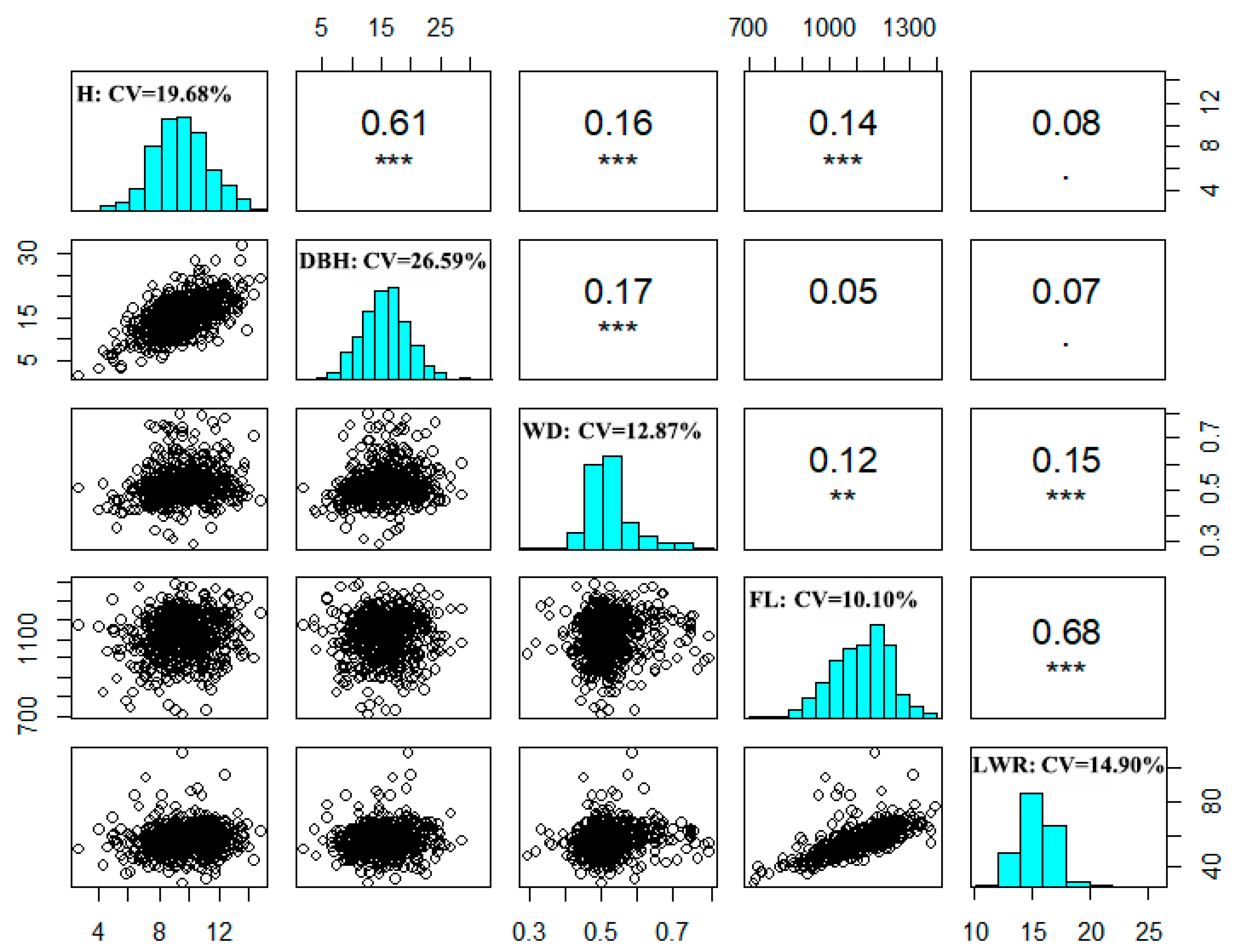
The descriptive statistical results of growth and wood traits of 226 clones in the reference population are shown in
Figure 1, the diagonal histogram plots indicated that all five traits nearly obeyed a normal distribution. The coefficients of variation of growth traits were higher than those of wood traits, among them, the coefficient of variation of DBH was highest (26.59%), and the coefficient of variation of FW was lowest (10.10%). Moreover, the Pearson correlation coefficients between the five traits were almost significantly positive, among them, the highest one was between FL and LWR ( r=0.68,
P<0.001). Interestingly, there is significantly positive correlated between WD and growth traits, indicating that we may improve WD and growth traits simultaneously.
3.2. Statistics of Genotyping Data
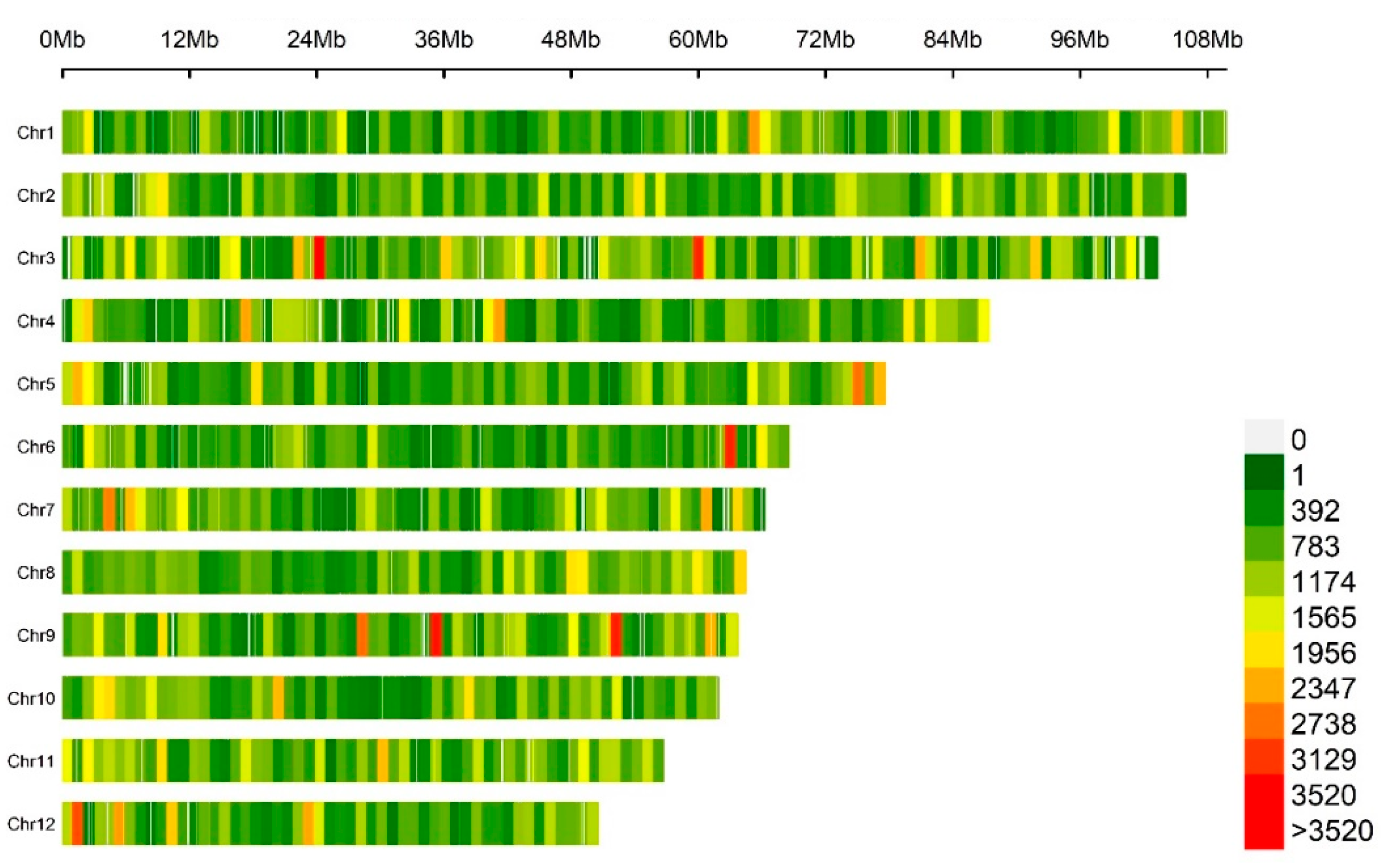
After quality control, the distribution of SNPs on the
C. hystrix genome was relatively uniform (
Figure 2), and two regions in both Chr3 and Chr9 and one region in Chr6, had a large marker density, greater than 3500 SNP•Mb
-1. As shown in
Table 1, Chr1 was the longest with a length of about 110 Mb and had a marker density of 760 SNP•Mb
-1, while Chr12 was the shortest with a length of about 51 Mb and a marker density was 904 SNP•Mb
-1. The marker density of all chromosomes ranged from 760 to 954 SNP•Mb
-1, the highest was Chr9 (954.18 SNP•Mb
-1), the lowest was Chr1 (760.13 SNP•Mb
-1), and the average marker density was about 870 SNP•Mb
-1.
3.3. Effect of Varying the Number of SNPs on the Estimates of Heritability
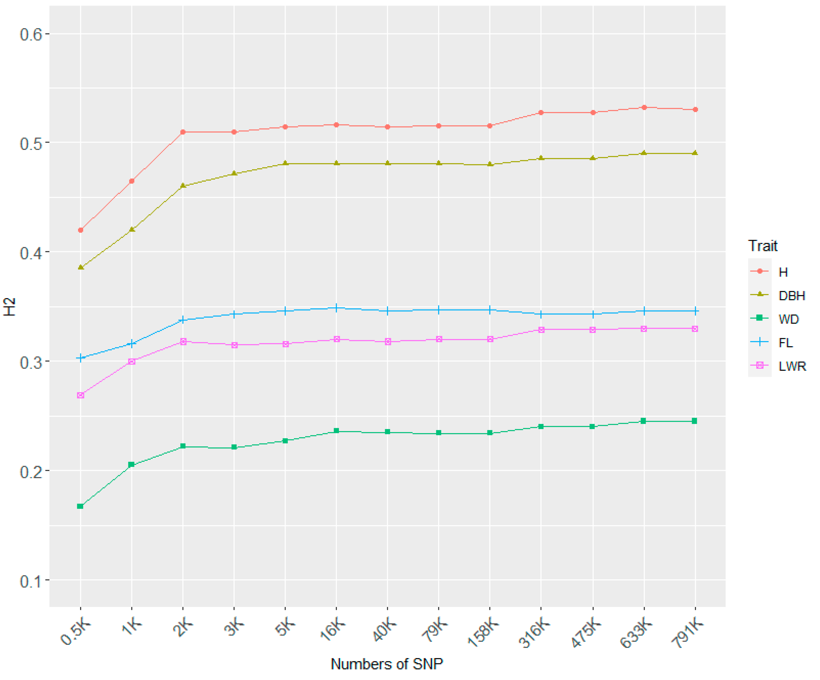
To evaluate the impact of varying the number of SNPs on the estimates of heritability, we used the GBLUP model, the results showed that the 13 different numbers of SNPs had little effect on broad-sense heritability (
Figure 3). Heritabilities increased slightly and reached a plateau around 5K SNPs for all traits. The highest heritability was H (around 0.5), followed by DBH (around 0.48), and the lowest one was WD (around 0.25). The broad-sense heritabilities of growth traits were higher than those of wood quality traits.
3.4. Effect of Varying Number of SNPs on the GS Prediction Accuracy
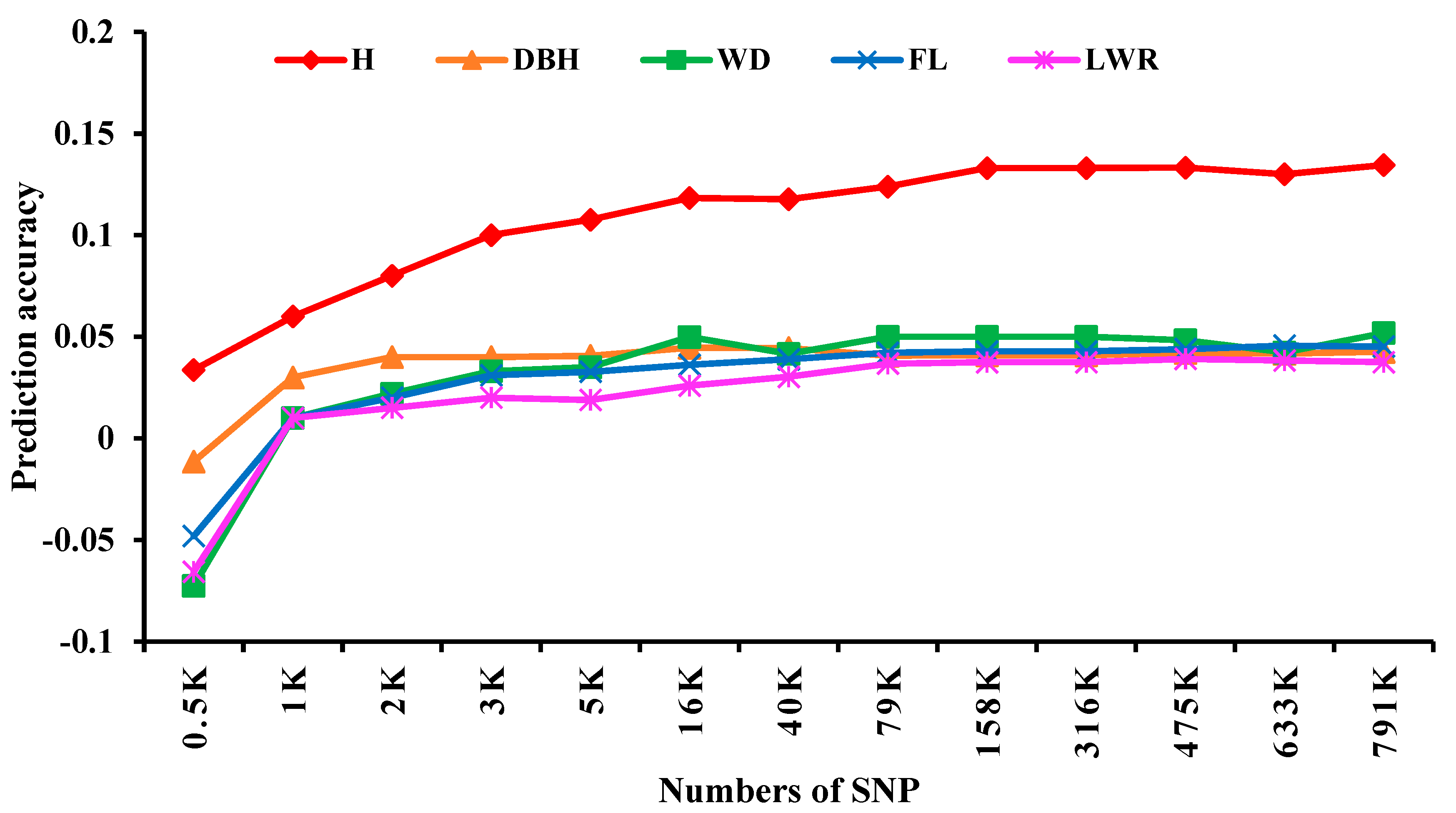
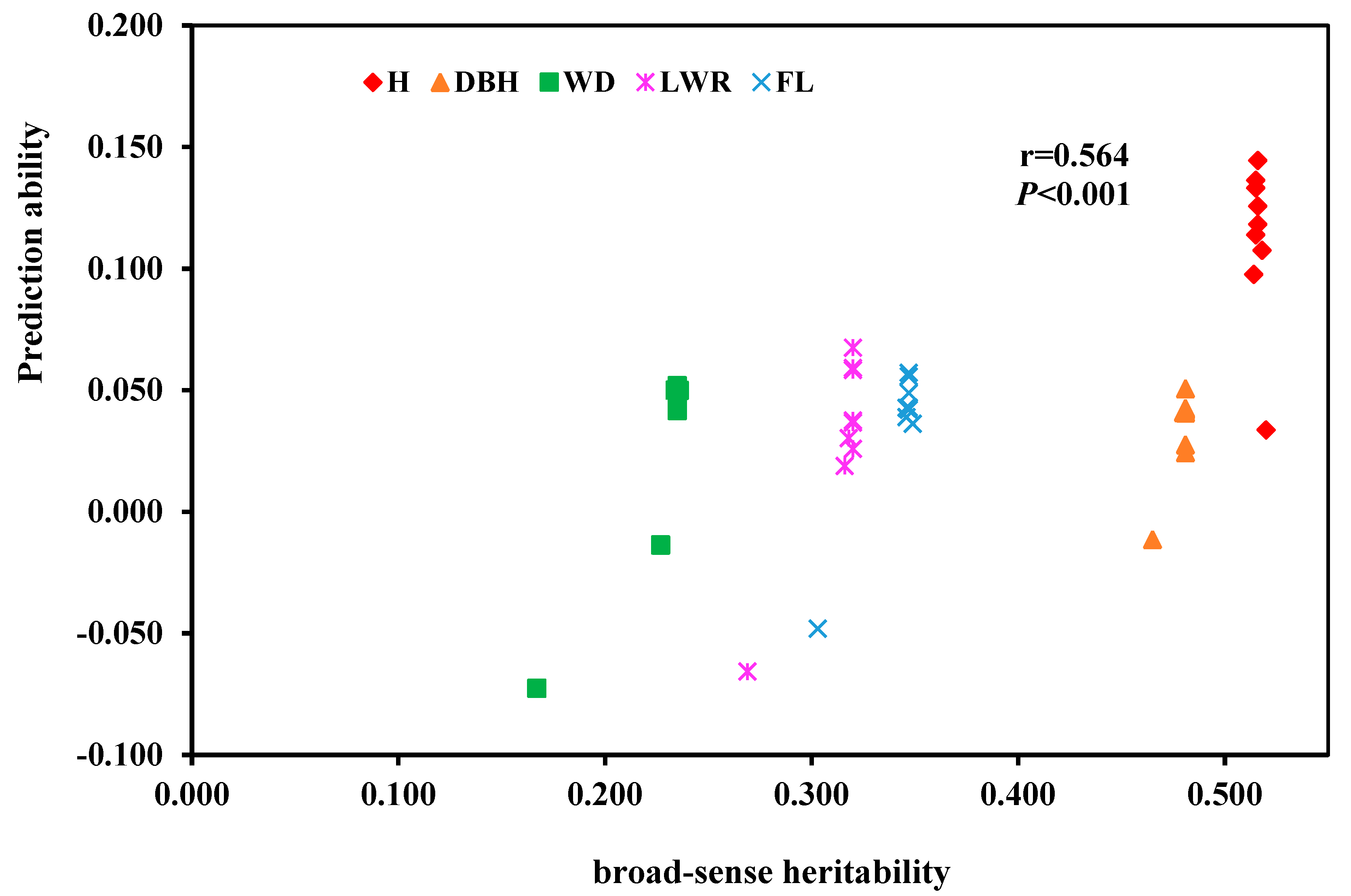
The effect of different SNP numbers on GS prediction accuracy was studied with the Bayes C model, the results showed that PA first increased and then reached a plateau around 3K SNPs for all traits (
Figure 4). Further comparison of prediction accuracy showed that the PA of H was higher than those of the other four traits and that the other four traits had similar GS prediction accuracy. The results of Pearson correlation analysis (
Figure 5) showed that there was a significant positive correlation (r=0.564,
P<0.001) between the broad-sense heritability of these five traits and their GS predictive ability.
3.5. Effect of Varying Statistics Models on the GS Prediction Accuracy
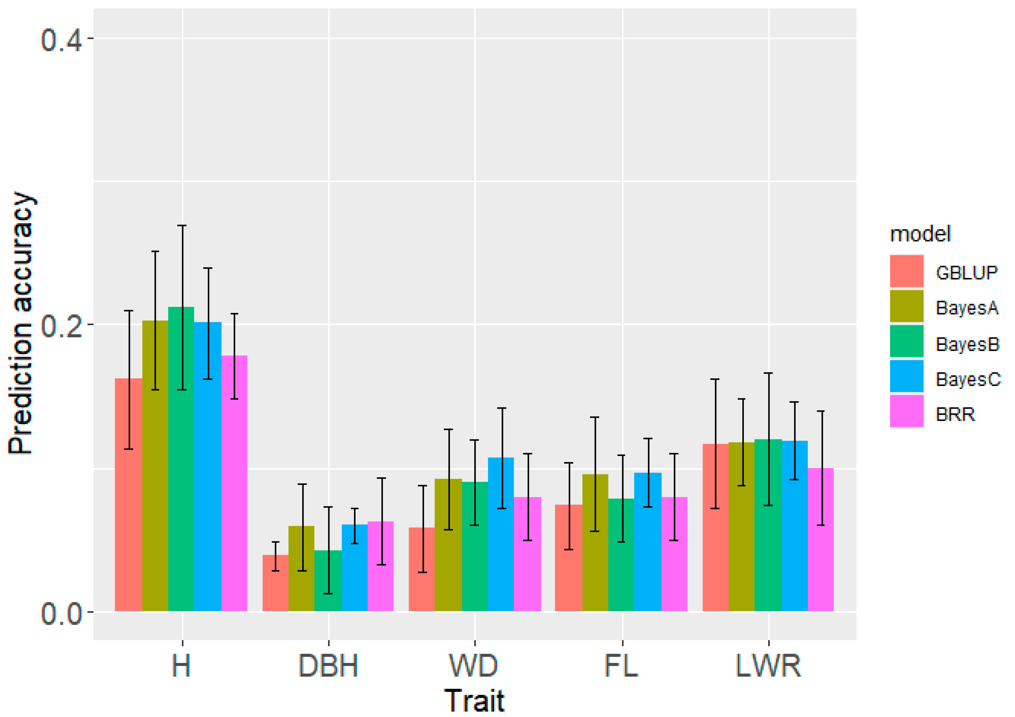
As shown in
Figure 6, the prediction accuracy of four Bayesian models was better than that of GBLUP. However, there was little difference between the Bayesian models, and the Bayes C model was the highest and relatively robust. GS of H had the highest PA, followed by wood quality traits, and their PA was close.
3.6. Early Selection of Superior Progeny Individuals in the Candidate Population
Based on the above comparison results of the different SNP numbers on the broad-sense heritability estimation and the prediction accuracy of GS, 5K SNPs were selected for the comprehensive selection of superior offspring. The top 15 superior progeny individuals were selected with a 3% selection rate. As shown in
Table 2, the Q
i value of these 15 selected progeny individuals ranged from 2.195 to 2.213, belonging to 7 families, of which F5 was the most, accounting for 26.7%, followed by F6 and F11, accounting for 20%, respectively. The mean GEBVs of the selected individuals almost exceeded the mean phenotypic values of the reference population, and their genetic gain ranged from 0.319% to 2.671%.
4. Discussion
4.1. Effect of Trait Heritability on GS Prediction Ability
Some studies have shown a positive correlation between trait heritability and GS predictive ability [
10,
15,
33]. For example, Estopa et al. declared that the heritability of carbohydrate content was the highest and its GS predictive ability was also the highest in
E. benthamii, while the heritability of volume was relatively tiny and its predictive ability of GS was also weak [
33]. In this study, there was a significant positive correlation between the generalized heritability of tree height and DBH traits and their GS predictive ability (r=0.859,
P<0.001). However, Cao et al. reported that there was no significant correlation between the heritability of traits and their GS predictive ability in peach [
34]. Therefore, the effect of trait heritability on its GS predictive ability may be related to species and trait types. In addition, the number of SNP markers in the range of 3K~791K had little effect on the broad-sense heritability of the five traits, similar to the results of
E. benthamii [
33], indicating that when the number of SNPs reached a certain number, the number of SNPs had little effect on the heritability estimation.
4.2. Effect of Varying Number of SNPs on the GS Prediction Accuracy
Many studies have shown that the prediction accuracy of GS increases with the increase of the number of SNP markers, but when reaching a certain number, the prediction accuracy of GS tends to stabilize and reaches a plateau [
13,
33]. Nsibi et al. found that when the number of SNPs was less than 6,103 (10% of the total markers), the prediction accuracy continued to increase, and then the increase in the number of SNPs had little effect on the prediction accuracy [
35]. Estopa et al. reported that the GS predictive ability of all traits in
E. benthamii reached a plateau after the number of SNPs reached 3K [
33]. Herein, the GS prediction accuracy was lowest when the number of SNPs was 0.5K, and the reason may be due to the lower SNP density reducing the degree of linkage between SNP markers and QTLs, thus resulting in decreasing the GS prediction accuracy. However, it has also been reported that increased SNP labeling density can sometimes cause some noise that affects the accuracy of GEBV estimation [
36]. The reasons may be: (1) the increase in SNP marker density adds a large number of markers that are not related to the target trait, which interferes with the estimation of GEBV, and then affects the prediction accuracy of GEBV to some extent; (2) the number of markers is much larger than the sample size, which may lead to model overfitting.
4.3. Effect of Varying Statistics Models on the GS Prediction Accuracy
Different traits have different genetic structures, and different statistical models should be used to evaluate the prediction efficiency [
37]. Isik et al. observed similar GS prediction abilities of GBLUP, BRR, and Bayes LASSO (BL) in growth and trunk straightness traits in maritime pine, while when using the BL model, the prediction ability was higher, but the prediction bias was also larger [
11]. In another study of maritime pine, the prediction accuracy of ABLUP was higher than that of GBLUP or BL [
28]. In
E. benthamii, the prediction ability of the six GS models for all target traits was similar, but all of them were better than the ABLUP model [
33]. Our results show that the prediction accuracy of the Bayesian models for the same trait is very close, but it is higher than that of the GBLUP model, indicating that the assumptions of the Bayes models have little effect on the GS prediction. Nevertheless, when more complex external environmental factors are considered, such as the statistics model accounting for external spatial effects and competitive effects, GBLUP model may present its advantages for complex models [
38].
4.4. The Efficiency of GS Early Selection
One significant advantage of GS is that it can greatly shorten the breeding cycle [
18]. For example, in dairy cows [
39], GS shortened the breeding cycle from 7 years to 1 year and increased genetic gain by 35%, while in rice [
40], GS increased rice yield by 16% compared to the traditional cross-breeding. In this study, the genetic gain of the five traits of the 15 selected individuals ranged from 0.319% to 2.671%, compared with the reference population, regardless of the selection period. Assuming that the selection period is shortened from 16 years to 2 years, the genetic gain will increase by 7 times. However, the prediction accuracy of GS in this study was still not high, which was lower than the average prediction accuracy (0.45) in the reported GS studies of forest trees [
18]. The reasons may be as follows: (1) The reference population is tiny. Bartholome et al. suggested that the reference population should be greater than 2000 trees [
28]. (2) The relationship between individuals in the reference population is weak. Isik reported that the GS prediction accuracy of full-sib family was significantly higher than that of half-sib family [
18]. Our reference population in this study came from six provenances, and their genomic relationship matrix values were generally small. Therefore, in the future, half-sib and full-sib families should be added to the reference population and the GS prediction should be re-evaluated.
5. Conclusions
In this study, GS prediction model for growth and wood traits in C. hystrix was established, and the effects of different SNP numbers and statistical models on the prediction accuracy of GS were also analyzed. The Bayes models had better prediction accuracy than the GBLUP model, and the number of SNPs had a limited effect on the GS prediction accuracy, consistent with the results of GS studies in other forest trees. Meanwhile, the early selection of superior individuals was carried out according to the GEBVs of growth and wood traits of the candidate population, which laid a technical and material foundation for the rapid breeding of excellent new varieties of C. hystrix. In addition, the prediction accuracy of GS in our research was not high, therefore the reference population should be enlarged and re-evaluated in the future.
Author Contributions
Conceptualization, writing—review and editing, Y.L.; methodology, W.Z.; software, R.W.; supervision, Y.L. and W.Z.; formal analysis, R.W. and W.Z.; visualization, R.W. All authors have read and agreed to the published version of the manuscript.
Funding
This research was funded by the Key-Area Research and Development Program of Guangdong Province, with project numbers 2020B020215002.
Data Availability Statement
The data presented in this study are available on request from the corresponding author.
Conflicts of Interest
The authors declare no conflicts of interest.
References
- Meuwissen, T.; Hayes, B.; Goddard, M. Prediction of total genetic value using genome-wide dense marker maps. Genetics 2001, 157, 1819–1829. [Google Scholar] [CrossRef] [PubMed]
- Isik, F.; Holland, J.; Maltecca, C. Genetic data analysis for plant and animal breeding. Springer International Publishing: Switzerland, 2017.
- VanRaden, P. Efficient methods to compute genomic predictions. J. Dairy Sci. 2008, 91, 4414–4423. [Google Scholar] [CrossRef] [PubMed]
- Beyene, Y.; Semagn, K.; Mugo, S.; Tarekegne, A.; Babu, R.; Meisel, B.; Sehabiague, P.; Makumbi, D.; Magorokosho, C.; Oikeh, S. Genetic gains in grain yield through genomic selection in eight bi-parental maize populations under drought stress. Crop Sci. 2015, 55, 154–163. [Google Scholar] [CrossRef]
- Spindel, J.; Begum, H.; Akdemir, D.; Virk, P.; Collard, B.; Redoña, E.; Atlin, G.; Jannink, J.; McCouch, S. Genomic selection and association mapping in rice (Oryza sativa): effect of trait genetic architecture, training population composition, marker number and statistical model on accuracy of rice genomic selection in elite, tropical rice breeding lines. PLOS Genetics 2015, 11, e1004982. [Google Scholar]
- Resende, M.; Resende, M.; Sansaloni, C.; Petroli, C.; Missiaggia, A.; Aguiar, A.; Abad, J.; Takahashi, E.; Rosado, A.; Faria, D.; Pappas, G.; Kilian, A.; Grattapaglia, D. Genomic selection for growth and wood quality in Eucalyptus: capturing the missing heritability and accelerating breeding for complex traits in forest trees. New Phytol. 2012, 194, 116–128. [Google Scholar] [CrossRef] [PubMed]
- Duran, R.; Isik, F.; Zapata-Valenzuela, J.; Balocchi, C.; Valenzuela, S. Genomic predictions of breeding values in a cloned Eucalyptus globulus population in Chile. Tree Genet. Genomes 2017, 13, 74. [Google Scholar] [CrossRef]
- Rambolarimanana, T.; Ramamonjisoa, L.; Verhaegen, D.; Tsy, J.; Jacquin, L.; Cao-Hamadou, T.; Makouanzi, G.; Bouvet, J. Performance of multi-trait genomic selection for Eucalyptus robusta breeding program. Tree Genet. Genomes 2018, 14, 17. [Google Scholar] [CrossRef]
- Suontama, M.; Klápště, J.; Telfer, E.; Graham, N.; Stovold, T.; Low, C.; McKinley, R.; Dungey, H. Efficiency of genomic prediction across two Eucalyptus nitens seed orchards with different selection histories. Heredity 2019, 122, 370–379. [Google Scholar] [CrossRef] [PubMed]
- Resende, M.; Muñoz, P.; Resende, M.; Garrick, D.; Fernando, R.; Davis, J.; Jokela, E.; Martin, T.; Peter, G.; Kirst, M. Accuracy of genomic selection methods in a standard data set of loblolly pine (Pinus taeda L.). Genetics 2012, 190, 1503–1510. [Google Scholar] [CrossRef]
- Isik, F.; Bartholomé, J.; Farjat, A.; Chancerel, E.; Raffin, A.; Sanchez, L.; Plomion, C.; Bouffier, L. Genomic selection in maritime pine. Plant Sci. 2016, 242, 108–119. [Google Scholar] [CrossRef]
- Beaulieu, J.; Doerksen, T.; Clément, S.; MacKay, J.; Bousquet, J. Accuracy of genomic selection models in a large population of open-pollinated families in white spruce. Heredity 2014, 113, 343–352. [Google Scholar] [CrossRef] [PubMed]
- Chen, Z.; Baison, J.; Pan, J.; Karlsson, B.; Andersson, B.; Westin, J.; García-Gil, M.; Wu, H. Accuracy of genomic selection for growth and wood quality traits in two control-pollinated progeny trials using exome capture as the genotyping platform in Norway spruce. BMC Genomics 2018, 19, 946. [Google Scholar] [CrossRef] [PubMed]
- Thistlethwaite, F.; Ratcliffe, B.; Klápště, J.; Porth, I.; Chen, C.; Stoehr, M.; El-Kassaby, Y. Genomic prediction accuracies in space and time for height and wood density of Douglas-fir using exome capture as the genotyping platform. BMC Genomics 2017, 18, 930. [Google Scholar] [CrossRef] [PubMed]
- Kwong, Q.; Ong, A.; The, C.; Chew, F.; Tammi, M.; Mayes, S.; Kulaveerasingam, H.; Yeoh, S.; Harikrishna, J.; Appleton, D. Genomic selection in commercial perennial crops: applicability and improvement in oil palm (Elaeis guineensis Jacq.). Sci. Rep. 2017, 7, 1–9. [Google Scholar] [CrossRef]
- Cros, D.; Mbo-Nkoulou, L.; Bell, J.; Oum, J.; Masson, A.; Soumahoro, M.; Tran, D.; Achour, Z.; Guen, V.; Clement-Demange, A. Within-family genomic selection in rubber tree (Hevea brasiliensis) increases genetic gain for rubber production. Ind. Crop. Prod. 2019, 138, 111464. [Google Scholar] [CrossRef]
- O’Connor, K.; Hayes, B.; Hardner, C.; Alam, M.; Henry, R.; Topp, B. Genomic selection and genetic gain for nut yield in an Australian macadamia breeding population. BMC Genomics 2021, 22, 370. [Google Scholar] [CrossRef] [PubMed]
- Isik, F. Genomic Prediction of Complex Traits in Perennial Plants: A Case for Forest Trees. Methods Mol Biol. 2022, 2467, 493–520. [Google Scholar]
- Xu, F.; Liao, H.; Yang, X.; Pan, W.; Yang, H. The climatic regionalization of the distributional region of Castanopsis hystrix. For. Environ. Sci. 2017, 33, 21–28, [in Chinese with English abstract]. [Google Scholar]
- Li, N.; Yang, Y.; Xu, F.; Chen, X.; Li, Z.; Wei, R.; Pan, W.; Zhang, W. Phenotypic variation study and comprehensive selection of elite clonal populations of Castanopsis hystrix. J. Cent. South Univ. For. Techn. 2023, 43, 73–84, [in Chinese with English abstract]. [Google Scholar]
- Zhu, J.; Jiang, Y.; Pan, W. Study on the selection criteria of Castanopsis hystrix superior tree in Guangxi. Guangxi For. Sci. 2002, 3, 109–113, [in Chinese with English abstract]. [Google Scholar]
- Yang, H.; Liao, H.; Yang, X.; Zhang, W.; Pan, W. Genetic variation analysis of growth and form traits of Castanopsis hystrix in the second generation seed orchard. J. South China Agr. Univ. 2017, 38, 81–85, [in Chinese with English abstract]. [Google Scholar]
- Liu, G.; Tian, Z.; Jia, H.; Shen, W.; Li, Z.; Tang, L.; Zhao, H.; Xu, J. Genetic parameter estimates for the growth and morphological traits of Castanopsis hystrix families and the genotype× environment interaction effects. Forests 2023, 14, 1619. [Google Scholar] [CrossRef]
- Wang, M.; Tu, Z.; Qiu, X.; Zhu, J.; Jiang, Y.; Ye, Z. Genetic diversity of Castanopsis hystrix by RAPD analysis. J. Xiamen Univ. 2006, 4, 570–574, [in Chinese with English abstract]. [Google Scholar]
- Li, N.; Yang, Y.; Xu, F.; Chen, X.; Wei, R.; Li, Z.; Pan, W.; Zhang, W. Genetic diversity and population structure analysis of Castanopsis hystrix and construction of a core collection using phenotypic traits and molecular markers. Genes 2022, 13, 2383. [Google Scholar] [CrossRef]
- Lin, Y.; Yang, H.; Ivkovic, M.; Gapare, W.; Matheson, C.; Wu, H. Effect of genotype by spacing interaction on radiata pine wood density. Aust. For. 2014, 77, 203–211. [Google Scholar] [CrossRef]
- Danecek, P.; Auton, A.; Abecasis, G.; Albers, C.; Banks, E.; DePristo, M.; Handsaker, R.; Lunter, G.; Marth, G.; Sherry, S.; McVean, G.; Durbin, R. 1000 Genomes Project Analysis Group. The variant call format and VCFtools. Bioinformatics 2011, 27, 2156–2158. [Google Scholar] [CrossRef] [PubMed]
- Bartholome, J.; Van Heerwaarden, J.; Isik, F.; Boury, C.; Vidal, M.; Plomion, C.; Bouffier, L. Performance of genomic prediction within and across generations in maritime pine. BMC Genomics 2016, 17, 604. [Google Scholar] [CrossRef]
- Xiao, L.N.; Wei, R.; Tan, Z.; Zhang, W.; Lin, Y. AFEchidna is a R package for genetic evaluation of plant and animal breeding datasets. For. Environ. Sci. 2022, 38, 50–56, [in Chinese with English abstract]. [Google Scholar]
- Pérez-Enciso, M.; Rincón, J.; Legarra, A. Sequence- vs. chip-assisted genomic selection: accurate biological information is advised. Genet. Sel. Evol. 2015, 47, 43. [Google Scholar] [CrossRef]
- Legarra, A.; Robert-Granié, C.; Manfredi, E.; Elsen, J. Performance of genomic selection in mice. Genetics 2008, 180, 611–618. [Google Scholar] [CrossRef]
- Ding, C.; Huang, Q.; Zhang, B.; Chu, Y.; Zhang, W.; Su, X. Evaluation of important traits of different clones of north-typed Populus deltoides. For. Res. 2016, 29, 331–339. [Google Scholar]
- Estopa, R.; Paludeto, J.; Müller, B.; Oliveira, R.; Azevedo, C.; Resende, M.; Tambarussi, E.; Grattapaglia, D. Genomic prediction of growth and wood quality traits in Eucalyptus benthamii using different genomic models and variable SNP genotyping density. New Forests 2023, 54, 343–362. [Google Scholar] [CrossRef]
- Cao, K.; Chen, C.; Yang, X.; Bie, H.; Wang, L. Genomic selection for fruit weight and soluble solid contents in peach. Scientia Agr. Sinica 2023, 56, 951–963, [in Chinese with English abstract]. [Google Scholar]
- Nsibi, M.; Gouble, B.; Bureau, S.; Flutre, T.; Sauvage, C.; Audergon, J.; Regnard, J. Adoption and optimization of genomic selection to sustain breeding for apricot fruit quality. G3 (Bethesda) 2020, 10, 4513–4529. [Google Scholar] [CrossRef] [PubMed]
- Perez, P.; Delos, C. Genome-wide regression and prediction with the BGLR statistical package. Genetics 2014, 198, 483–495. [Google Scholar] [CrossRef] [PubMed]
- Crossa, J.; Pérez-Rodríguez, P.; Cuevas, J.; Montesinos-López, O.; Jarquín, D.; deLos Campos, G.; Burgueño, J.; González-Camacho, J.; Pérez-Elizalde, S.; Beyene, Y.; Dreisigacker, S.; Singh, R.; Zhang, X.; Gowda, M.; Roorkiwal, M.; Rutkoski, J.; Varshney, R. Genomic selection in plant breeding: methods, models, and perspectives. Trends Plant Sci. 2017, 22, 961–975. [Google Scholar] [CrossRef] [PubMed]
- Lin, Y.Z. Research methodologies for genotype by environment interactions in forest trees and their applications. Scientia Silvae Sinicae 2019, 55, 142–151. [Google Scholar]
- Xu, Y.; Liu, X.; Fu, J.; Wang, H.; Wang, J.; Huang, C.; Prasanna, B.; Olsen, M.; Wang, G.; Zhang, A. Enhancing genetic gain through genomic selection: from livestock to plants. Plant Commun. 2020, 1, 100005. [Google Scholar] [CrossRef]
- Hickey, J.; Chiurugwi, T.; Mackay, I.; Powell, W. Genomic prediction unifies animal and plant breeding programs to form platforms for biological discovery. Nat. Genet. 2017, 49, 1297–1303. [Google Scholar] [CrossRef]
|
Disclaimer/Publisher’s Note: The statements, opinions and data contained in all publications are solely those of the individual author(s) and contributor(s) and not of MDPI and/or the editor(s). MDPI and/or the editor(s) disclaim responsibility for any injury to people or property resulting from any ideas, methods, instructions or products referred to in the content. |
© 2024 by the authors. Licensee MDPI, Basel, Switzerland. This article is an open access article distributed under the terms and conditions of the Creative Commons Attribution (CC BY) license (http://creativecommons.org/licenses/by/4.0/).
