1. Introduction
Diagnostic Electro-myographic (D-EMG) Signals are used to detect and analyse electrical activity produced by muscles during contraction. EMG signals are typically acquired using surface electrodes placed on the skin above the muscles of interest. Signal processing techniques, including filtering and feature extraction, are then applied to extract relevant information for the analysis of relevant muscle inherent dynamics during a particular action or movements [
1,
2].
Muscle dynamics analysis with EMG holds significant clinical relevance, particularly in diagnosing and monitoring neuromuscular disorders. Advancements in EMG technology and signal processing techniques have expanded the scope of muscle dynamics analysis [
3].Abnormalities in muscle activation patterns, fatigue profiles, and coordination can indicate underlying pathologies, aiding in disease diagnosis and treatment evaluations [
4].
Nonlinear methods in D-EMG signal muscle inherent dynamics analysis offer a promising avenue for unraveling the complexities of muscle function. Their application holds significant potential for enhancing our understanding of motor control mechanisms, neuromuscular disorders, and rehabilitation strategies, ultimately contributing to improved clinical outcomes and patient care [
6,
7,
8,
9].
Patient-specific analysis of electromyography (EMG) signals using nonlinear methods offers several advantages in understanding individualized muscle dynamics and informing personalized treatment strategies [
10,
11,
12]. Patient-specific abnormalities in signal complexity, entropy, or recurrence dynamics may serve as biomarkers for disease diagnosis and monitoring. By involving patients in the analysis and interpretation of their EMG data, personalized approaches foster greater engagement and adherence to treatment plans. Empowering patients with insights into their own muscle dynamics encourages active participation in rehabilitation activities and promotes self-management strategies.
This article is organized as follows:
Section 2 describes the methodologies with Subsection’s, Subsection 2.1 include details such as demographics of participants, data collection procedures, and relevant ethical considerations. Subsection 2.2 focuses on testing the stationarity of the data using a Q-Q plot. Subsection 2.3, involves analyzing surrogate data, reconstructed using delay-coordinate embed- ding, Subsection 2.5, of the study likely discusses how the Poincar´e map is constructed from the reconstructed phase space and its implications for understanding the system’s dynamics, stability, and periodic behaviour. Subsection 2.6, the computation of the largest Lyapunov exponent from Poincar´e maps contributes to understanding the dynamic behavior of the system under study, particularly its chaotic or regular nature.
Section 3 discusses the observations and results obtained from the methodologies described in the
Section 2, in subsequent subsections. Finally, conclusions and future aspects of the study has been discussed.
2. Methodology
2.1. Participants Information and Data Collection
A male participant, age 22 years, weight 70 kg, height 5’ 7” (170.2 cm), was chosen for the present study under guided supervision and consent that the was not having any prior musculoskeletal injury which may lead to obstruction of the load pull task and a written consent for participation in the research activity. Non-invasive, disposable D-EMG electrode pairs are positioned parallel to the muscle of interest, such as the forearm, lateral-deltoids, biceps-bracci, and triceps-bracci, with a 0.2 m inter-electrode spacing, in accordance with the guidelines outlined in [
5,
13,
14,
15]. D-EMG collected using RMS EMG Recorder Aleron 201/401* (2/4 channel acquisition).
2.2. Test of Non Stationarity of Acquired D-EMG Signal using Quantile-Quantile (Q-Q) Plot and Augmented Dickey Fuller Test (ADF-Test)
Acquired D-EMG Signal is a time series data by its nature of acquisition, thus Non-Stationarity test assesses variability of the acquired signal’s statistical property (like mean and variance) over time. Plotting each of the quantiles of two probability distributions against one another enables statisticians to compare the distributions of variables using a graphical tool called a quantile-quantile (Q-Q) plot. The ADF-Test, also known as the Augmented Dickey Fuller Test, determines whether a time series with one variable is non-stationary by evaluating the existence of a unit root. If the null hypothesis (presence of a unit root) is rejected, it suggests stationary. By combining Quantile-Quantile (Q- Q) plot and the ADF test methods, one can gain a more nuanced understanding of the characteristics of the time series data and the potential presence of non-stationary [
16,
17,
18].
2.3. Surrogate Data Analysis (99% Confidence Interval)
The Test of Non-linearity by Surrogate Data is a method used to determine whether a given time series exhibits nonlinear behaviour. This test compares the original time series with surrogate data generated by shuffling the time order of the series while preserving its statistical properties. The 99% confidence interval in this context implies that the likelihood of observing a significant difference between the original D-EMG data and surrogate data due to random chance alone is less than 1%. If the comparison between the original data and surrogate data falls outside this confidence interval, validates the presence of non-linear behavior of the recorded time series signal [
19,
20,
21,
22,
23].
2.4. Phase Space Reconstruction
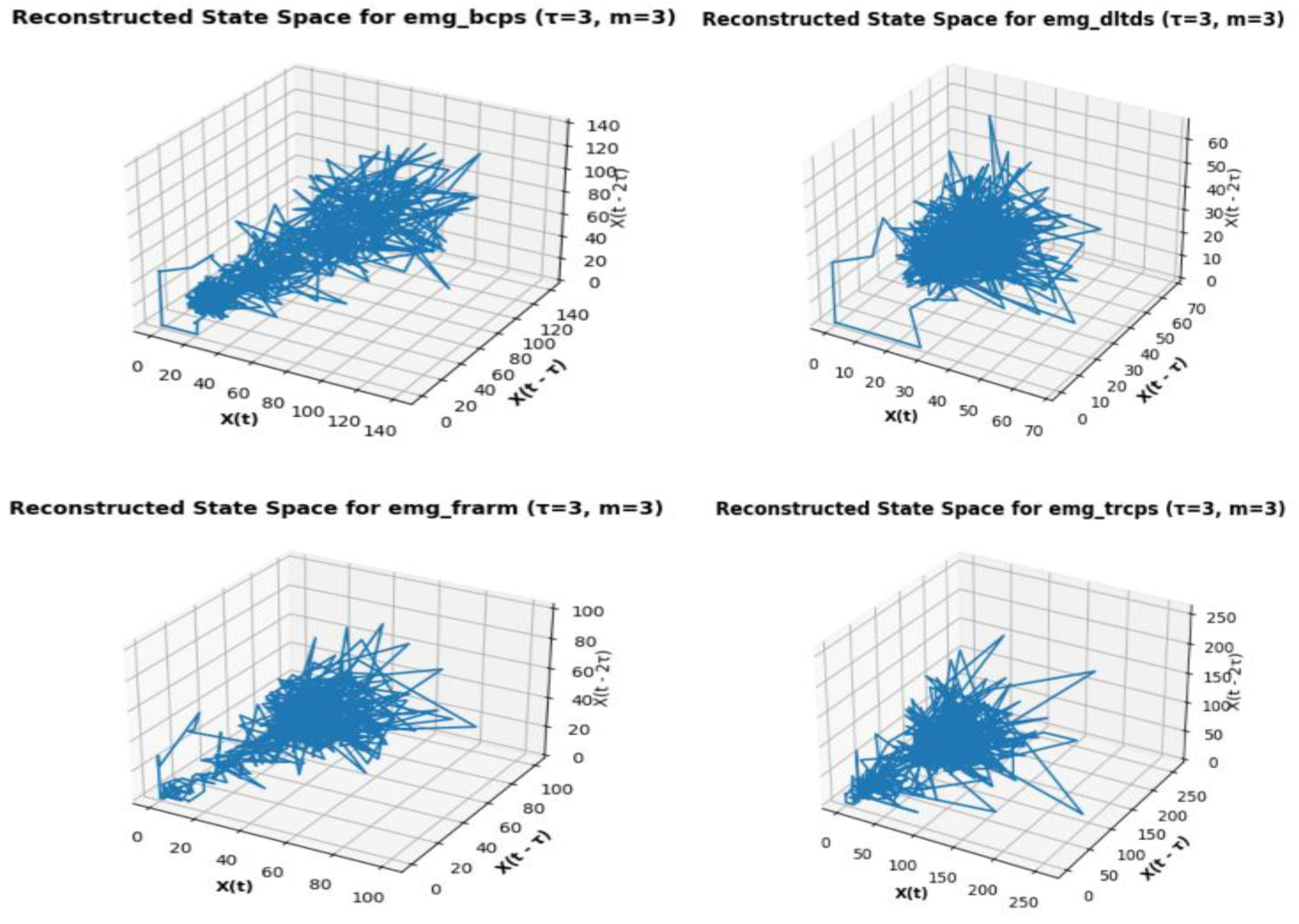
In the study of data driven nonlinear dynamics, phase space reconstruction is a method for analyzing the dynamics of a system from a time series of data. The goal is to use the phase space, a higher-dimensional space, to embed the D-EMG time series and rebuild the system’s underlying dynamics [
29]. Considering the D-EMG time series,
,embedded vectors is defined as,
where, τ is the time delay and m is the embedding dimension [
24,
25,
26,
27].
For each embedded vector
, computation of Average Mutual Information between neighboring points in the reconstructed phase space,
Where,
, is the number of nearest neighbour used in the calculation and
is the mutual information between embedded vectors
. The optimal values for m and τ can be determined by searching for values that maximize the criterion, such as the average mutual information, indicating that neighboring points in the reconstructed phase space contain significant information about each other [
28,
30,
31,
32].
2.6. Recurrence Quantification Analysis (RQA) of the Phase Space Reconstructed Set
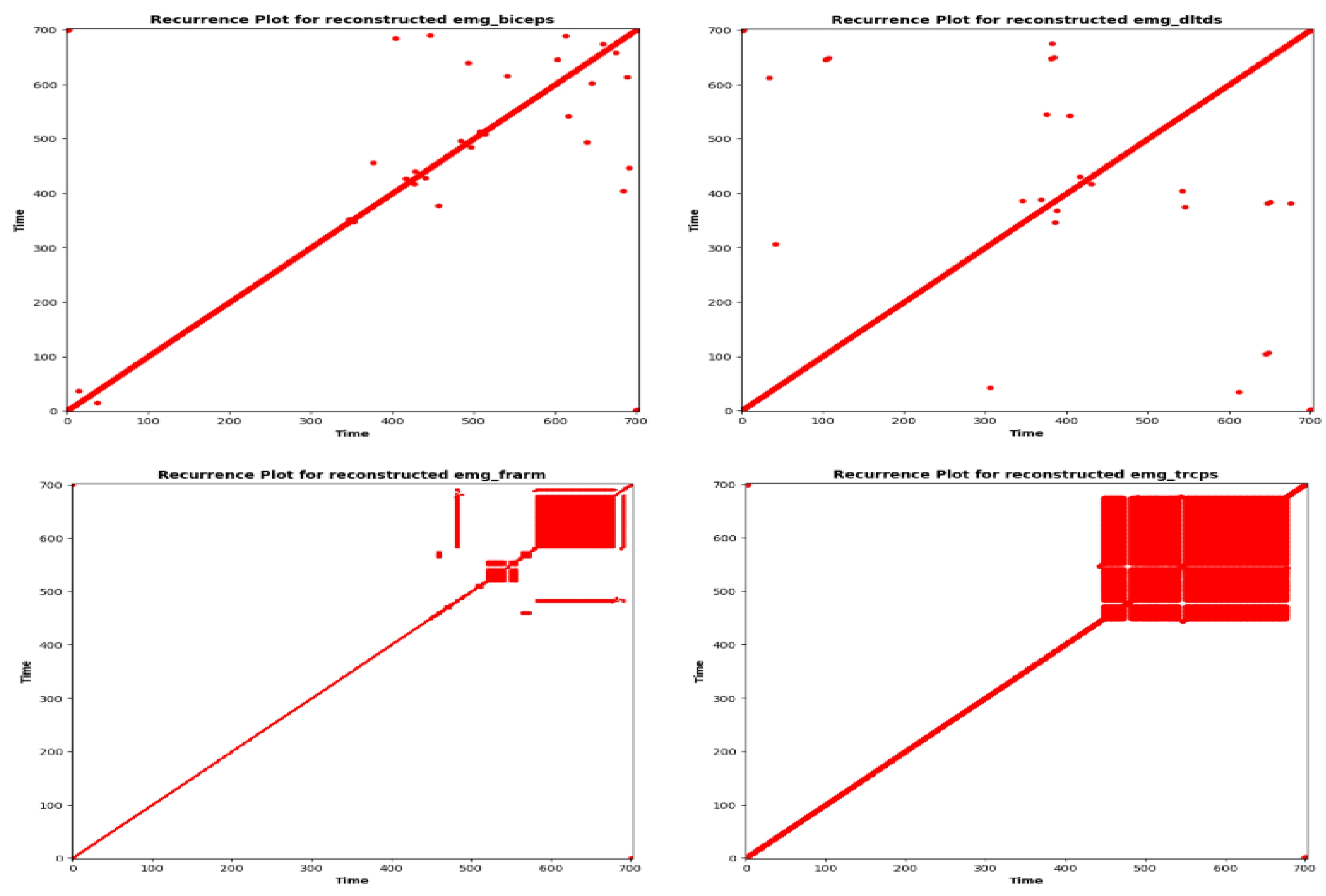
Recurrent Quantification Analysis (RQA), a method for analyzing the recurrence properties of a dynamical system, is widely used with D-EMG time series data. By quantifying recurrence plots, Recurrence Quantification Analysis (RQA) of D-EMG data evaluates patterns of muscle activity. RQA offers insights into the temporal dynamics and intricacy of EMG signals, while the plot illustrates the recurrent states within the phase space. If two states in the phase space are close to each other (i.e., their distance is below a certain threshold), they are considered recurrent. RQA involves the calculation of various quantification measures from the recurrence plot to characterize the system’s dynamics. Some commonly used measures includes:
Recurrence Rate (RR): The percentage of pairs that recur in the phase space. Recurrence rate calculation simplified equation:
where R(i,j) is the recurrence matrix, equal to 1 if points i and j are recurrent, and 0 otherwise. N is the number of points in the phase space.
Determinism (DET): The proportion of repeated points that create diagonal lines on the recurrence plot. Equation for evaluating DET:
Average Diagonal Line Length (AvgL): Average diagonal line length in recurrence plot.
Entropy (ENTR): The Shannon entropy of the distribution of diagonal line lengths.
Laminarity (LAM): The proportion of repeated points in a recurrence plot that form vertical lines.
RQA offers important insights into the predictability, complexity, and stability of the system’s underlying dynamics. It might be useful to comprehend the patterns and features of muscle activation in the context of EMG data [
33,
34,
35].
2.7. Poincar’e Map Construction From Phase Space Reconstructed Set
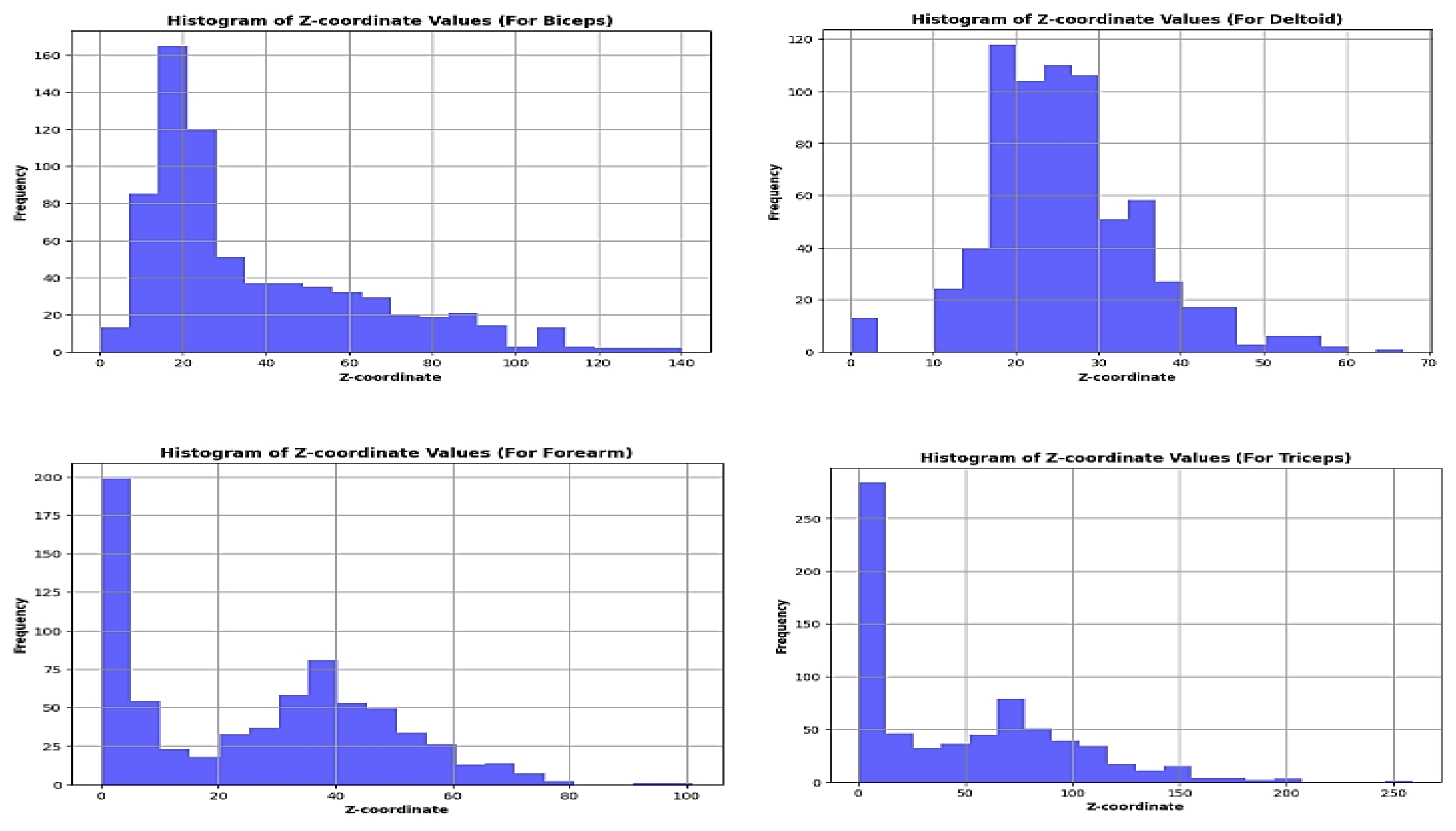
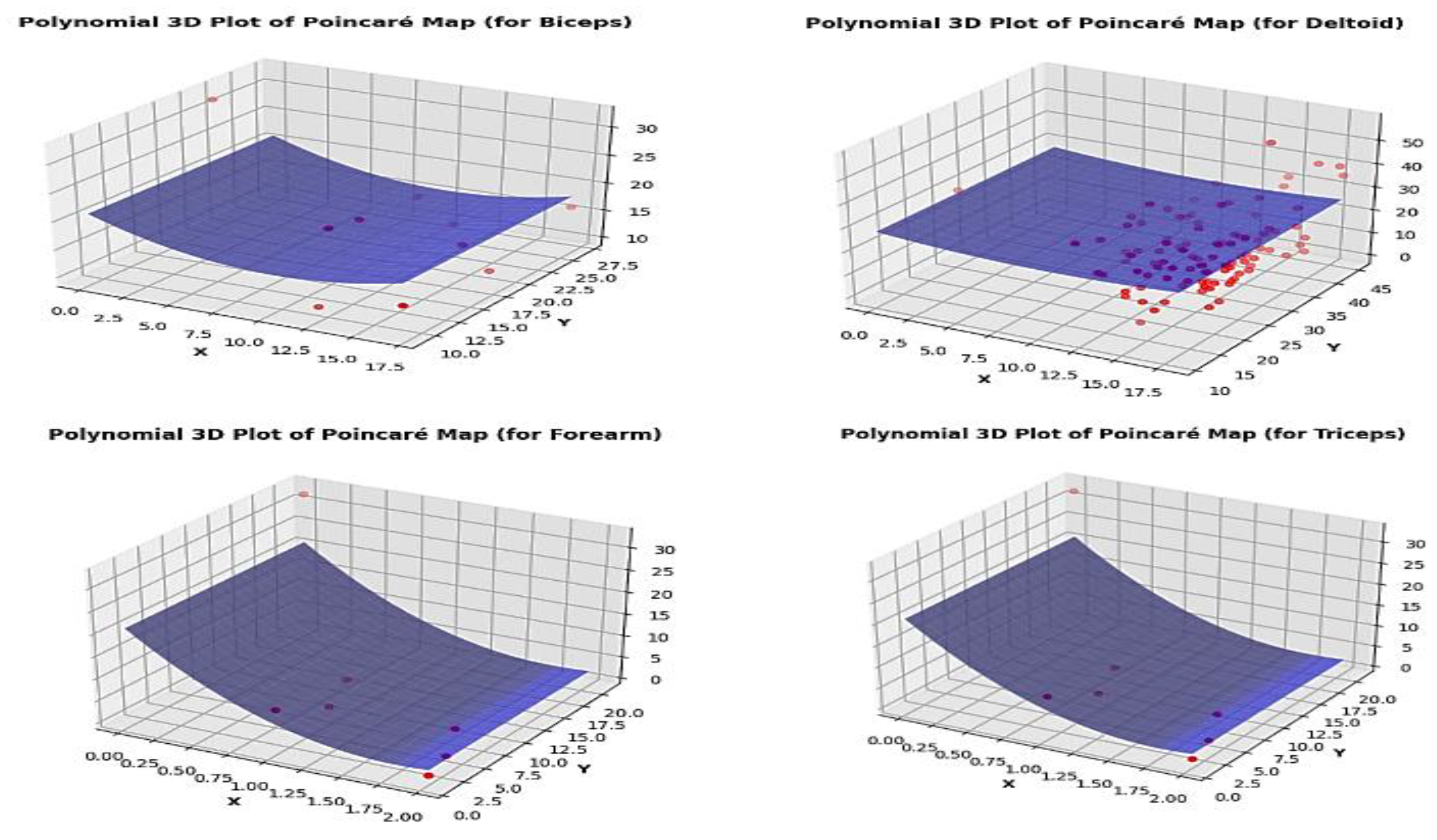
Once the phase space is reconstructed, a Poincar’e map can be constructed by intersecting trajectories in the phase space with a particular surface, often referred to as the Poincar’e section. The Poincar’e map is typically defined by fixing one or more variables in the phase space and observing the crossings of trajectories with this surface. Each intersection point offers a discrete representation of the system dynamics, representing the state of the system at a specific instant in time. For the experiment set, tracing these positions at the intersections on the plane of section is difficult. The lack of a dynamical equation to calculate the intersections plane’s crossing z-plane locations is the cause of this. Making a histogram of the z-coordinate values in the phase space that has been rebuilt is one method of tackling the problem. Examine the histogram for any peaks or clusters that might point to areas where the route spends more time. Select a z-coordinate value that is close to a notable cluster’s center or peak. A three-dimensional surface that fits the distribution of points on the Poincar’e map is represented by the polynomial 3D plot of the Poincar’e map that has been created. The consistency and smoothness of the surface reveal details about the dynamics and stability of the system. Smooth surfaces are indicative of stable systems, whereas morecomplicated or fractured surfaces could point to chaotic or unstable ones [
36,
37].
2.8. Largest Lyapunov Exponent from Poincar’e Map
The Largest Lyapunov Exponent (LLE) extracted from a Poincar’e map provides valuable information about the chaotic behavior and sensitivity to initial conditions within a dynamical system [
38,
39,
40]. This involves selecting a hyperplane (or a section) in the reconstructed phase space and recording the intersections of trajectories with this hyperplane. For each point on the Poincar’e map, calculate the distance between neighboring trajectories. This is typically done using some norm (e.g., Euclidean distance). Use the distances between neighboring trajectories to calculate the Lyapunov exponents. For the largest Lyapunov exponent, the formula can be simplified as follows:
Where,
is the distance between neighboring trajectories after i iterations and
is the initial distance between [
40].
3. Results and Discussion
3.1. Outcomes of Non Stationarity Test
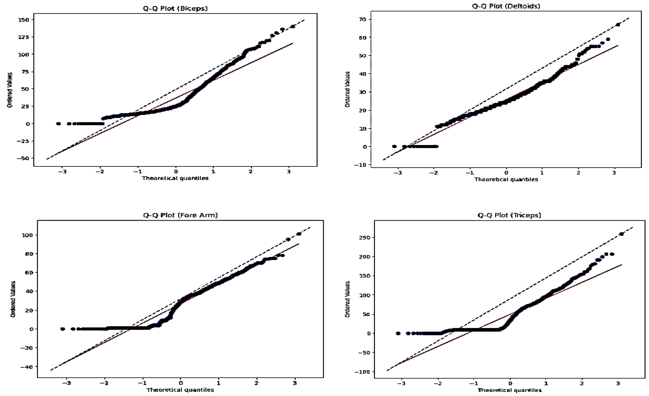
Figure 2 Shows the Q-Q plot, from the visual inspection the points deviate upwards or downwards from the diagonal dashed line (forming an S-curve shape), it suggests that the tails of the distribution in the data are heavier or lighter than expected under the theoretical distribution. This indicate non-stationarity, such as excess kurtosis (fat tails) or skewness.
Table 1., Analytical findings from the ADF test for Biceps Muscle show that the test statistic is (-1.0547). The test statistic in this instance is below the critical values at all common levels (1%, 5%, and 10%), indicating that the null hypothesis cannot be ruled out. The test statistic’s corresponding p-value is 0.7328. A high p-value indicates that there is insufficient evidence to reject the null hypothesis of non-stationarity. When rejecting the null hypothesis, one must consider the critical values as thresholds. The crucial values in this instance are given at the 1%, 5%, and 10% levels. The test statistic exceeds these crucial values, hence the null hypothesis of non-stationarity cannot be rejected. We conclude that there is not enough evidence to reject the null hypothesis of non-stationarity based on the results of the Dickey-Fuller test. This implies a non-stationary D-EMG series.
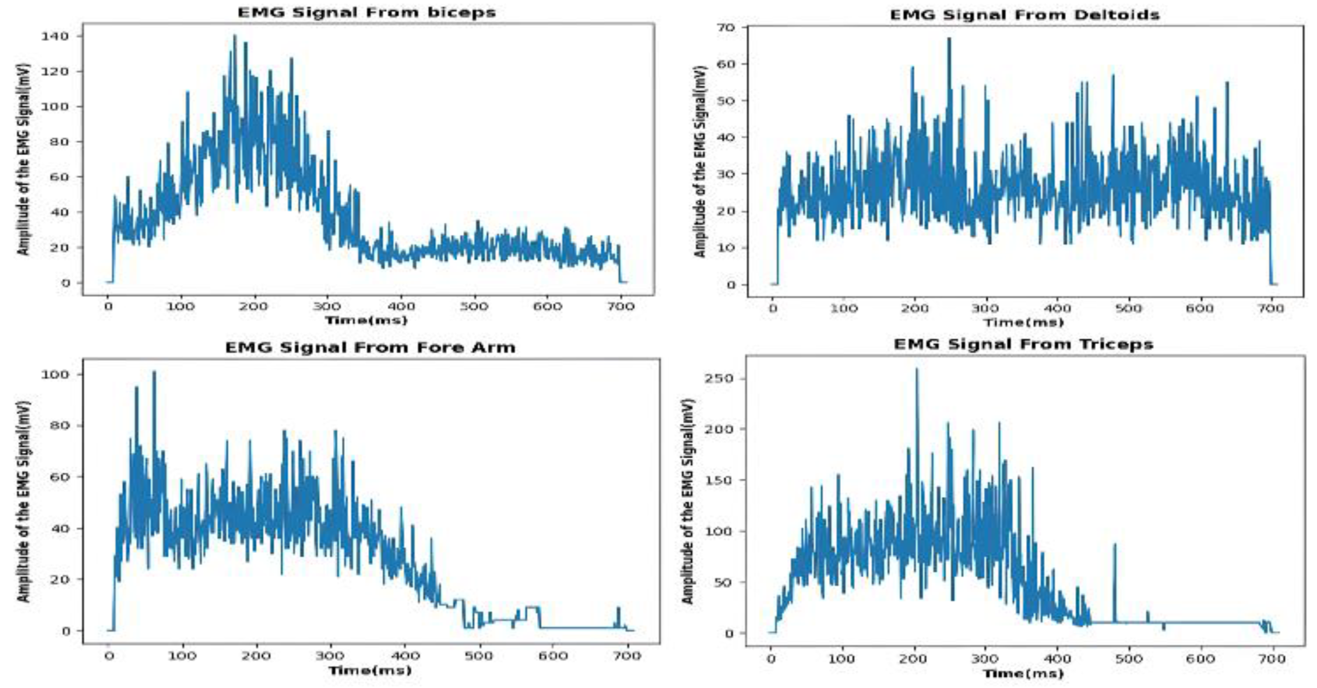
Figure 1.
Recorded D-EMG data for Biceps Bracci, Lateral Deltoid, Forearm and Triceps Bracci,from the participant (male, age 22 years, weight 70 kg, height 5’ 7”, (170.2 cm)).
Figure 1.
Recorded D-EMG data for Biceps Bracci, Lateral Deltoid, Forearm and Triceps Bracci,from the participant (male, age 22 years, weight 70 kg, height 5’ 7”, (170.2 cm)).
Figure 2.
Non Stationarity test of the each aquired D-EMG signal from the muscle using Q-Q plot.
Figure 2.
Non Stationarity test of the each aquired D-EMG signal from the muscle using Q-Q plot.
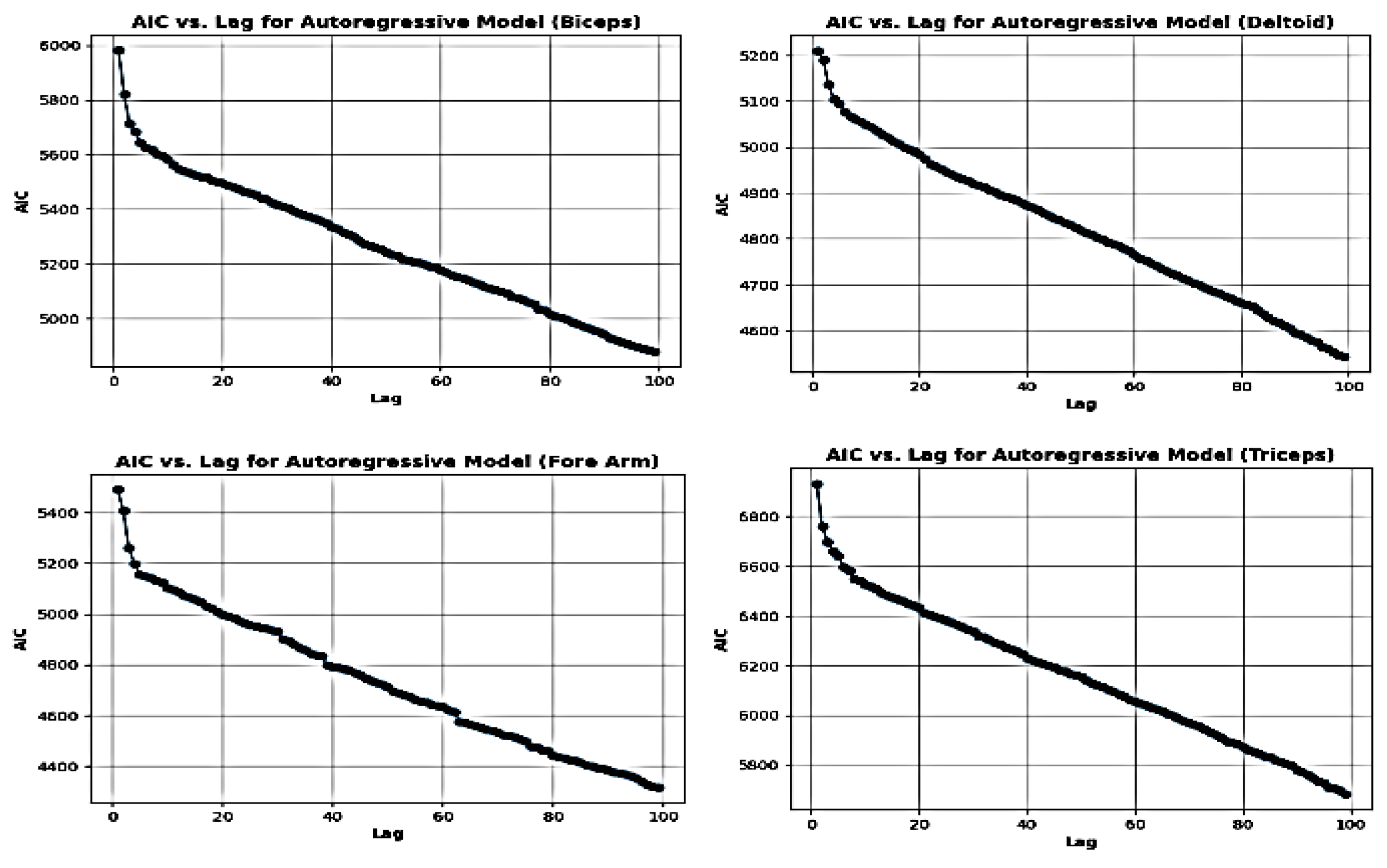
Figure 3.
Finding out optimal time delay (τ) from the aquired D-EMG signal for the phase space reconstrution.
Figure 3.
Finding out optimal time delay (τ) from the aquired D-EMG signal for the phase space reconstrution.
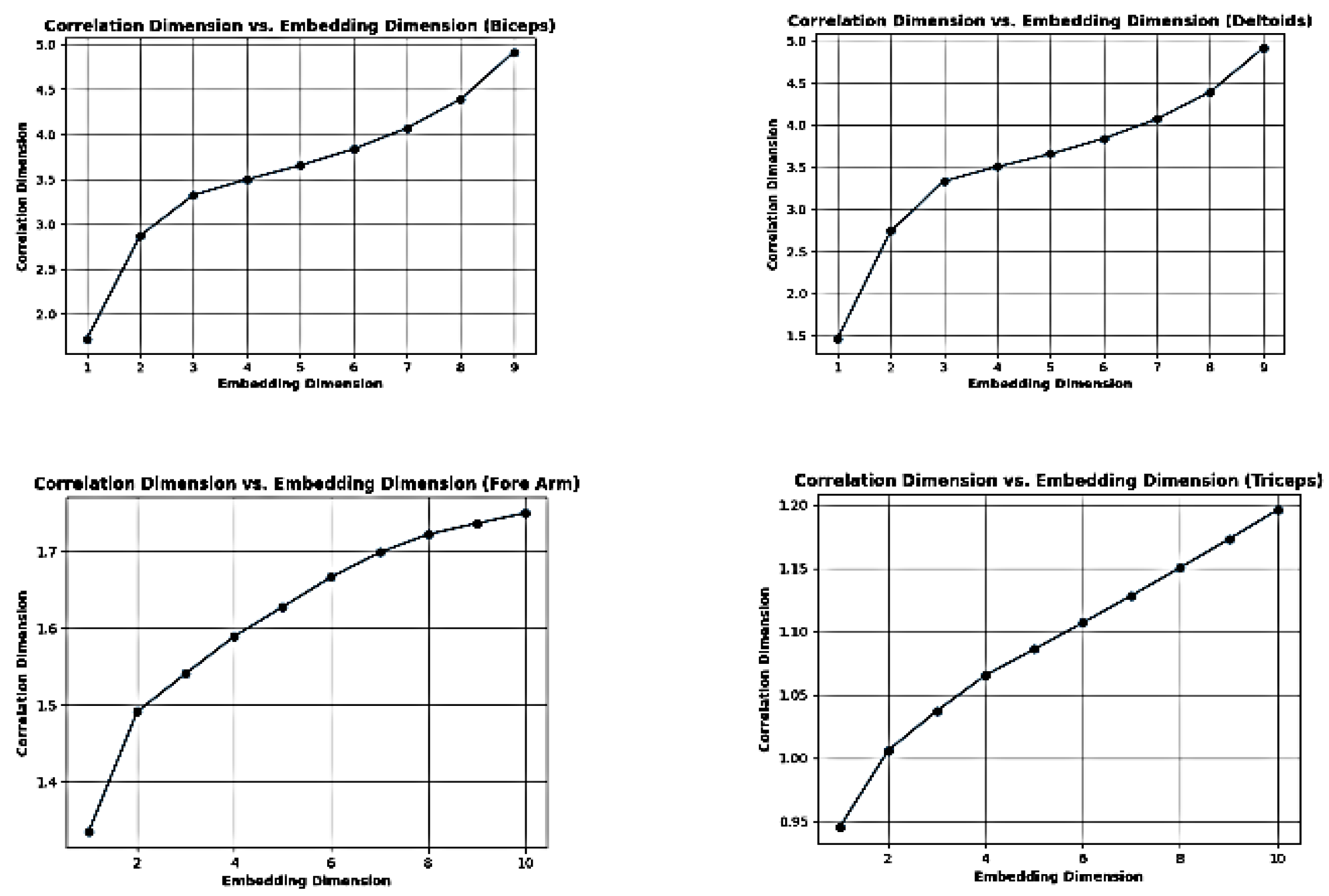
Figure 4.
Finding out optimal embedded dimension (ϵ) from the aquired D-EMG signal for the Phase Space Re- construction.
Figure 4.
Finding out optimal embedded dimension (ϵ) from the aquired D-EMG signal for the Phase Space Re- construction.
3.2. Outcomes of Surrogate Data Analysis
Table 2. Electromyography (EMG) data from the biceps, deltoids, forearm, and triceps were used as surrogate data for data analysis. This allowed for the determination of critical values at a 99% confidence level and the observation that the EMG data displayed nonlinear behavior. A p-value of 0.01 indicates that, in only 1% of circumstances, we would expect to see a test statistic that is as extreme as or more extreme than the one we observed if the null hypothesis were true (i.e., if the original time series were linear). The original time series is probably nonlinear as this number is less than a common significance threshold, such as 0.05, which leads us to reject the null hypothesis. The critical value is calculated at the 99% confidence level.
3.3. Outcomes of Recurrence Quantification Analysis
Each muscle exhibits unique recurrence quantification outcomes, suggesting variations in their dynamical properties. Forearm has the highest recurrence rate (0.836), indicating a higher frequency of revisiting previous states. Biceps Brachii has the lowest recurrence rate (0.0015), suggesting less repetition in its dynamics.Deltoids, Forearm, and Triceps show similar values for both determinism and laminarity, indicating comparable levels of deterministic behavior and laminar structures in their dynamics. Biceps Brachii has the lowest values for both determinism (0.0429) and laminarity (0.429), indicating less deterministic behavior and fewer laminar structures compared to the other muscles. Biceps Brachii exhibits the highest entropy. (6.477), indicating higher complexity or irregularity in its dynamics. Deltoids, Forearm, and Triceps show lower entropy values, suggesting relatively lower complexity compared to the Biceps Brachii muscle. he Biceps Brachii muscle appears to have less deterministic behavior, higher complexity, and longer recurrent patterns compared to the other muscles analyzed.
3.4. Analysis of Poincar’e Map
Considering
Figure 5,
Figure 6 and
Figure 7, For Biceps, At about 17.5, the histogram clearly demonstrates a peak. This implies that the z-coordinate in the phase space has a preferred value. A high-density point is seen close to the surface’s center on the Poincar’e map. This implies that the system contains an attractor. The 3D plot of the Poincar’e map shows a smooth and continuous surface. This suggests that the system is stable. Regarding Deltoids, The histogram exhibits a distinct peak at around 18.1. This implies that the z-coordinate in the phase space has a preferred value. A high-density point is seen close to the surface’s center on the Poincar’e map. This implies that the system contains an attractor. For Triceps, The histogram shows a clear peak at around 6.475. This implies that the z-coordinate in the phase space has a preferred value. A high-density point is seen close to the surface’s center on the Poincar’e map. This implies that the system contains an attractor. The Poincar’e map’s three-dimensional layout displays a continuous, smooth surface. This implies that stability inside the system. A distinct peak can be seen in the forearm histogram at about 2.525. This implies that the z-coordinate in the phase space has a preferred value.A high-density point is seen close to the surface’s center on the Poincar’e map. This implies that the system contains an attractor. The Poincar’e map’s three-dimensional layout displays a continuous, smooth surface. This implies that stability inside the system. Overall, the analysis of the plots suggests that all four muscles exhibit stable behavior with attractors in their phase spaces.
3.5. Analysis of Poincar’e Map
Table 4, The largest Lyapunov exponents from the poincare maps of phase space reconstructed for the triceps, biceps, forearm, and deltoids are 0.3199, 0.26, 0.121, and 0.10098, respectively. These values represent the rate of divergence or convergence of nearby trajectories in the reconstructed phase space, providing insights into the system’s dynamical behavior. The deltoids exhibit the highest complexity among the analyzed muscle groups, with a Lyapunov exponent of 0.18. This suggests that the dynamics of the deltoids during the observed motion are more chaotic or unpredictable compared to the other muscles. The differences in Lyapunov exponents among muscles may reflect variations in coordination and synchronization. Lower Lyapunov exponents (biceps with 0.12) indicate more ordered and synchronized motion, whereas higher exponents (deltoids with 0.18) suggest greater variability and less synchronization between muscle groups. Analyzing the dynamical properties of muscle activity could provide valuable insights into movement disorders or rehabilitation processes. Monitoring changes in Lyapunov exponents could help assess the effectiveness of interventions or track progression in conditions affecting neuromuscular control.
4. Conclusions
This study has provided valuable insights into the muscle dynamics during exercise activity through a participant specific analysis. By utilizing various analytical techniques, including stationarity tests, surrogate data analysis, phase space reconstruction, Recurrance Quantification Analysis (RQA) Poincar’e map formulation, and calculation of the largest Lyapunov exponent, the non-linear and chaotic nature of electromyography (EMG) signals has been explored. The findings suggest that the muscle dynamics exhibit complex behavior, characterized by non-stationarity and chaotic dynamics. This implies that traditional linear models may not fully capture the intricacies of muscle activity during exercise. Understanding these dynamics is crucial for improving the accuracy of models.Future works in this area could focus on several aspects. Firstly, further exploration of different exercise modalities and muscle groups could provide a comprehensive understanding of muscle dynamics across various contexts.Moreover, longitudinal studies tracking muscle dynamics over extended periods could reveal insights into the adaptive processes and effects in the dynamics of exercise on muscle function.
Funding
This research received no external funding
Informed Consent Statement
Informed consent was obtained from all subjects involved in the study.
Data Availability Statement
The datasets used in this research are available upon reasonable request. Please contact corresponding author or Contributing Authors for access to the data available at GitHub repository link provided in the Supplementary section.
Conflicts of Interest
The authors declare no conflicts of interest.
References
- B.Rodr’ıguez-Tapia, I. B.Rodr’ıguez-Tapia, I. Soto, D. M. Mart’ınez and N. C. Arballo, ”Myoelectric Interfaces and Related Applications: Current State of EMG Signal Processing–A Systematic Review,” in IEEE Access, vol. 8, pp. 7792-7805, 2020. [CrossRef]
- Gohel V, Mehendale N. Review on electromyography signal acquisition and processing. Biophys Rev. 2020 Nov 10;12(6):1361–7. [CrossRef]
- Raez MB, Hussain MS, Mohd-Yasin F. Techniques of EMG signal analysis: detection, processing, classification and applications. Biol Proced Online. 2006;8:11-35. [CrossRef]
- Martinek, R.; Ladrova, M.; Sidikova, M.; Jaros, R.; Behbehani, K.; Kahankova, R. ; Kawala-Sterniuk,A. Advanced Bioelectrical Signal Processing Meth- ods: Past, Present, and Future Approach—PartIII:Other Biosignals.Sensors, 2021, 21, 6064. [Google Scholar] [CrossRef]
- Pritam Chakraborty, Biswarup Neogi Achintya Das— Zhongmin Jin (Reviewing editor) (2020) Knowledge Based database of arm-muscle and activity characterization during load pull exercise using Diagnostic Electromyography (D-EMG) Signal., Cogent Engineering,7:1. [CrossRef]
- M. Lei and G. Meng, ‘Nonlinear Analysis of Surface EMG Signals’, Computational Intelligence in Electromyography Analysis - A Perspective on Current Applications and Future Challenges. InTech, Oct. 17, 2012. [CrossRef]
- Vivian, M. , Tagliapietra, L., Reggiani, M., Farina, D., Sartori, M. (2014). Design of a Subject-Specific EMG Model for Rehabilitation Movement. In: Jensen, W., Andersen, O., Akay, M. (eds) Replace, Repair, Restore, Relieve – Bridging Clinical and Engineer- ing Solutions in Neurorehabilitation. Biosystems & Biorobotics, vol 7. Springer, Cham.
- S. Ma, C. S. Ma, C. Chen, D. Han, X. Sheng, D. Farina and X. Zhu, ”Subject-Specific EMG Modeling with Multiple Muscles: A Preliminary Study,” 2020 42nd Annual International Conference of the IEEE En- gineering in Medicine Biology Society (EMBC), Montreal, QC, Canada, 2020, pp. 740-743. [CrossRef]
- Kugiumtzis, D. (2002). Surrogate Data Test on Time Series. In: Soofi, A.S., Cao, L. (eds) Modelling and Forecasting Financial Data. Studies in Computational Finance, vol 2. Springer, Boston, MA. [CrossRef]
- S. Yun, W. S. Yun, W. Ying, M. Xiangfei, Z. Fashun and G. Wen, ”Methodology of estimating the embedding dimension in chaos time series based on the prediction per formance of K-CV GRNN,” 2018 International Conference on Information Systems and Computer Aided Education (ICISCAE), Changchun, China, 2018,pp.
- H. L. Yap and C. J. Rozell, ”Stable Takens’ Embeddings for Linear Dynamical Systems,” (2011) in IEEE Transactions on Signal Processing, vol. 59, no. 10, pp. 4781- 4794, Oct. 2011.
- Y. Li, Z. Y. Li, Z. Chen and S. Cang, ”Phase Space Reconstruction and Time Series Prediction of a Nonlinear Financial System,” (2021) IEEE 10th Data Driven Control and Learning Systems Conference (DDCLS), Suzhou, China, 2021,pp.23-28. [CrossRef]
- W. D. Cai, Y. Q. W. D. Cai, Y. Q. Qin and B. R. Yang, ”Selection of Delay Time Window and Delay Time in Phase Space Reconstruction,” (2007) International Conference on Computational Intelligence and Secu- rity (CIS 2007), Harbin, China, 2007, pp. 526-530. [CrossRef]
- Ma, Hg. , Han, Cz. Selection of Embedding Dimension and Delay Time in Phase Space Reconstruction. ( 2006) Front. Electr. Electron. Eng. China 1, 111–114. [CrossRef]
- Matilla-Garc’ıa M, Morales I, Rodr’ıguez JM, Ruiz Mar’ın M. Selection of Embedding Dimension and Delay Time in Phase Space Reconstruction via Symbolic Dynamics. Entropy (Basel). 2021 Feb 11;23(2):221. [CrossRef]
- Wallot S, Roepstorff A, Mønster D. Multidimensional Recurrence Quantification Analysis (MdRQA) for the Analysis of Multidimensional Time-Series: A Software Implementation in MATLAB and Its Application to Group-Level Data in Joint Ac- tion. Front Psychol. 2016 Nov 22;7:1835. [CrossRef]
- Jackson ES, Tiede M, Riley MA, Whalen DH. Recurrence Quantification Analysis of Sentence-Level Speech Kinematics. J Speech Lang Hear Res. 2016 Dec 1;59(6):1315-1326. [CrossRef]
- 2017; 37. [CrossRef]
- K. M. Kafarov, S. S. K. M. Kafarov, S. S. Loginov and M. Y. Zuev, ”Modified Lorentz and Chua Systems Largest Lyapunov Exponent and Statistical Characteristics Analysis,” 2021 Systems of Signal Synchronization, Generating and Processing in Telecommunications(SYN-CHROINFO), Kaliningrad, Russia,2021. [CrossRef]
- Michael, T. Rosenstein, James J. Collins, Carlo J. De Luca, A practical method for calculating largest Lyapunov exponents from small data sets, Physica D: Nonlinear Phenomena, Volume 65, Is- sues 1–2, 1993, Pages 117-134,ISSN:0167-2789.
- Zayneb Brari, Safya Belghith, A new algorithm for Largest Lyapunov Exponent determination for noisy chaotic signal studies with application to Elec- troencephalographic signals analysis for epilepsy and epileptic seizures detection, Chaos, Solitons Fractals, Volume 165, Part 1, 2022, 112757, ISSN 0960-0779.
- Yanli Mengi, Bingzheng Liu and Yuping Liu, ”A comprehensive nonlinear analysis of electromyogram,” 2001 Conference Proceedings of the 23rd Annual International Conference of the IEEE En- gineering in Medicine and Biology Society, Is-tanbul, Turkey, 2001, pp.1078-1081 vol.2. [CrossRef]
- Hu, X. , Wu, Xb., Zou, B. et al. Nonlinear characteristics and functional analysis of masseter electromyography. J. Cent. South Univ. Technol. 18, 834–839 (2011). [CrossRef]
- Yanli Meng, Yuping liu and Bingzheng Liu, ”Test nonlinear determinacy of Electromyogram,” 2005 IEEE Engineering in Medicine and Biology 27th An- nual Conference, Shanghai, 2005, pp. 4592-4595. [CrossRef]
- Lachlan Winter, Paul Taylor, Clint Bellenger, Paul Grimshaw Robert G. Crowther (2023) The application of the Lyapunov Exponent to analyse human performance: A systematic review, Jour- nal of Sports Sciences, 41:22, 1994-2013. [CrossRef]
- 2023; 82. [CrossRef]
- Reza Yaghoobi Karimui, Sassan Azadi, Cardiac arrhythmia classification using the phase space sorted by Poincare sections, Biocybernetics and Biomedical Engineering, Volume 37, Issue 4, 2017, Pages 690-700,ISSN:0208-5216.
- K.M. Kafarov, S. S. K.M. Kafarov, S. S. Loginov and M. Y. Zuev, ”Modified Lorentz and Chua Systems Largest Lyapunov Exponent and Statistical Characteristics Analysis,” 2021 Systems of Signal Synchronization, Generat- ing and Processing in Telecommunications (SYN- CHROINFO, Kaliningrad, Russia, 2021, pp. 1-5. [CrossRef]
- Hong, WC. (2020). Phase Space Reconstruction and Recurrence Plot Theory. In: Hybrid Intelligent Tech- nologies in Energy Demand Forecasting. Springer,Cham. [CrossRef]
- S Claesen and R., I. Kitney, ”Estimation of the largest Lyapunov exponent of an RR interval and its use as an indicator of decreased autonomic heart rate control,” Computers in Cardiology 1994, Bethesda, MD, USA, 1994, pp. 133-136. [CrossRef]
- T. Michael, T. T. Michael, T. Rosenstein, James J. Collins, Carlo J. De Luca, A practical method for calculating largest Lyapunov exponents from small data sets, Physica D: Nonlinear Phenomena, Volume 65, Is- sues 1–2, 1993, Pages 117-134, ISSN 0167-2789. [CrossRef]
- Yanli Meng, Yuping liu and Bingzheng Liu, ”Test nonlinear determinacy of Electromyogram,” 2005 IEEE Engineering in Medicine and Biology 27th An- nual Conference, Shanghai, 2005, pp. 4592-4595. [CrossRef]
- Mondelli M, Aretini A, Greco G. Knowledge of elec- tromyography (EMG) in patients undergoing EMG examinations. Funct Neurol. 2014 Jul-Sep;29(3):195- 200. PMCID: PMC4264787. [PubMed]
- Filligoi G, Felici F. Detection of hidden rhythms in surface EMG signals with a non-linear time-series tool. Med Eng Phys. 1999 Jul-Sep;21(6-7):439-48. [CrossRef] [PubMed]
- 2023. [CrossRef]
- M.S. Singh, R. M.S. Singh, R. Pasumarthy and V. Talasila,”TimeSeries Analysis of Surface EMG Signal-Linear,Non Linear and Chaotic Approaches,” 2019 Fifth Indian Control Conference (ICC), New Delhi, India, 2019, pp.442-447.
- D. Farago, D. D. Farago, D. MacIsaac, M. Suk and A. D. C. Chan, ”A Review of Techniques for Surface Electromyog- raphy Signal Quality Analysis,” in IEEE Reviews in Biomedical Engineering, vol. 16, pp. 472-486, 2023. [CrossRef]
- McManus L, De Vito G, Lowery MM. Analysis and Biophysics of Surface EMG for Physiotherapists and Kinesiologists: Toward a Common Language With Rehabilitation Engineers. Front Neurol. 2020 Oct 15;11:576729. [CrossRef] [PubMed]
- F.H Khan, U. F.H Khan, U. Ashraf, M. A. Bin Altaf and W. Saadeh, ”A Patient-Specific Machine Learning based EEG Processor for Accurate Estimation of Depth of Anesthesia,” 2018 IEEE Biomedical Circuits and Systems Conference (BioCAS), Cleveland, OH, USA, 2018, pp. 1-4. [CrossRef]
- W. Wang, A. De. W. Wang, A. De. Stefano, R. 2006; 36. [Google Scholar] [CrossRef]
|
Disclaimer/Publisher’s Note: The statements, opinions and data contained in all publications are solely those of the individual author(s) and contributor(s) and not of MDPI and/or the editor(s). MDPI and/or the editor(s) disclaim responsibility for any injury to people or property resulting from any ideas, methods, instructions or products referred to in the content. |
© 2024 by the authors. Licensee MDPI, Basel, Switzerland. This article is an open access article distributed under the terms and conditions of the Creative Commons Attribution (CC BY) license (https://creativecommons.org/licenses/by/4.0/).
