1. Introduction
Topics such as aerodynamic forces easily appear in external flows. Then drag, lift, and lateral forces can emerge [
1]. When a fluid flow moves over a body at speeds higher than the speed of sound, another issue can be presented, shock waves [
2]. This sharp change of pressure can generate high drag and heat into the front of anybody which moves at supersonic or hypersonic speeds. Many of the geometries associated with these serious conditions are blunt bodies, e.g., missiles, space shuttles, and rockets [
3,
4,
5]. While it is true that streamlined bodies present better performance (i.e., a blunt body with a rounded or flat front end creates a stronger shock wave than a streamlined body, which has a pointed front end) blunt bodies are used due to questions of space [
6].
Supersonic flow over a blunt body is characterized by shock waves that form on the surface of the body and propagate downstream from it. In addition to the drag (pressures difference and viscous effect) and heat (compression of the gas in front of the shock wave) flow separation is observed. Flow separation occurs when the high-speed gas flowing over an object separates from the surface of the object, creating a region of low pressure behind it, which deflects the supersonic flow. The existence of such phenomena damages the body's surface and leads to a loss in aerodynamic performance [
7]. In this sense, several techniques have been developed to reduce the drag in supersonic flow, including geometric modifications on the object. One of these techniques consists of an extended body called a spike. A geometric spike is a pointed protrusion that extends from the nose of an object and commonly is aligned to the direction of flow [
8]. This aerodynamic body allows control of the flow and prevents separation. The spike creates an oblique shock wave (primary shock wave) that reduces the strength of the shock wave that originally would be formed on the surface of the blunt object (secondary shock wave). This primary shock wave reduces the strength of the secondary shock wave, which in turn reduces the amount of drag generated by the object [
9]. The effectiveness of a spike in reducing drag depends on several factors, including the angle and length of the spike, the Mach number of the flow, and the shape of the object [
10,
11,
12] In general, the spike should be long enough to generate a strong secondary shock wave, but not so long that it creates excessive drag on its own. It is important to note that the sharp leading edge of the spike also should be optimized to create the desired shock wave pattern, decrease the heating due to the concentration of shock waves, and maintain the stability at high speeds. At the same time, the shape of the blunt object should be designed to minimize the drag generated by the remaining shock wave [
8].
Major advances in the understanding of the use of the drag reduction mechanism by spikes have been produced through experimental and numerical studies, particularly through the CFD [
13,
14,
15,
16]. However, the fidelity of these works requires high computational resources and time, mainly when complex geometries or configurations are introduced. In aerospace engineering, rapid innovation is key and there lies a compelling need for more efficient methods without costly iterative simulations that may delay the rapid development and testing of novel aerodynamic configurations. In this sense, it is evident to explore alternative approaches to streamline and accelerate the design process.
In recent years, machine learning (ML) emerges as a promising complementary avenue with its capacity to learn from and make predictions on data. By harnessing versatile ML algorithms, attenuating the reliance on continuous CFD simulations is possible, thereby advancing a more efficient predictive framework for fluid flow phenomena and their effects, including aerodynamic properties. There are several articles that recognize the advantages and possibilities of machine learning [
17,
18]. Research areas of aeronautics [
19,
20], aeroacoustics [
21,
22,
23], combustion, resistance of materials [
24,
25] and manufacturing have benefited from the application of unsupervised learning. Particularly on the prediction of aerodynamic coefficients, using Neuronal Networks [
26,
27,
28] there is the work of Linse and Stengel [
26] applied to aircraft transport, with good results validated with flight tested data in the early 90's. The dynamic stall effect was performed by Suresh et al. [
27] at high angle of attack again with experimental data. Secco and Mattos [
28] studied the aerodynamic response of transport airplanes. Using a broad dataset generated by CFD simulations they trained a model and reduce by 4000 times the prediction of drag and lift coefficients. Recently, Ghoteyshi et al. [
29], Wang et al. [
30], and Hou et al. [
31], successfully tested the viability of these tools.
Despite of these promising methods, their implementation is often difficult due to the inherent complexities such as the need for extensive hyperparameter tuning, large training datasets, and advanced understanding of both the fluid mechanics and machine learning domains. In other words, accurate and accessible models to CFD practitioners without deep ML expertise are scarce. This gap beckons for a method that strikes a balance between predictive performance and ease of deployment. Among the many remarkable machine learning strategies, the K-Nearest neighbours (k-NN) algorithm emerges as a robust predicting tool renowned for its simplicity and effectiveness [
32]. The fidelity of this model is evidenced by its adaptability and scalability, with minimal need for retraining or extensive parameter adjustments.
The relevance of this work lies in the fact that after the literature review and despite of previous works have used CFD in combination with k-NN as prediction mechanism, it is not deeply explored way in supersonic flow ranges or applied to spike blunt bodies. Thereby, this work is aimed to drag coefficient prediction of a spike blunt body based the k-NN algorithm at velocities above the speed of sound (Mach numbers).
The rest of the paper is presented as follows: methodology, prototype geometry, numerical simulation, validation and dataset generation, results and discussion and conclusions.
2. Method
This section describes the necessary steps to test the effectiveness of the algorithm to calculate the drag coefficient of a spike blunt body, as well as the implementation of the calculation technique. A reliable and complete dataset is essential to provide information to the ML Algorithm. RANS simulations are performed in SolidWorks Software to obtain this dataset at different geometric and flow conditions. The simulated prototype geometry is the simplest spike blunt bodies. This proposal is to save computational resources and short generate-up times of data. Once the dataset is determined, the k-NN algorithm of Machine Learning Technique is implemented and applied.
2.1. Numerical Simulation and Validation
SolidWorks Flow Simulation Software is used to analyse this external compressible flow. To validate the effectiveness of the compressible flow code embodied in the software another simple geometry es selected, a sphere. The sphere is selected due there are several works reporting drag coefficients performance under sub to supersonic conditions [
33,
34].
Different mesh grids to ensure mesh independence are probed prior to validation. First, two grid meshes with distinct refinement levels, fine (553776 cells) and coarse (144952 cells) are used, and an adaptive mesh (2 refinement levels).
The main assumptions are homogeneous and isotropic material, adiabatic surface sphere and without heat transfer interaction. The external flow of the sphere is considered the baseline case for the validation of the code. Sphere and blunt body are analysed at the same thermal conditions, see
Table 1.
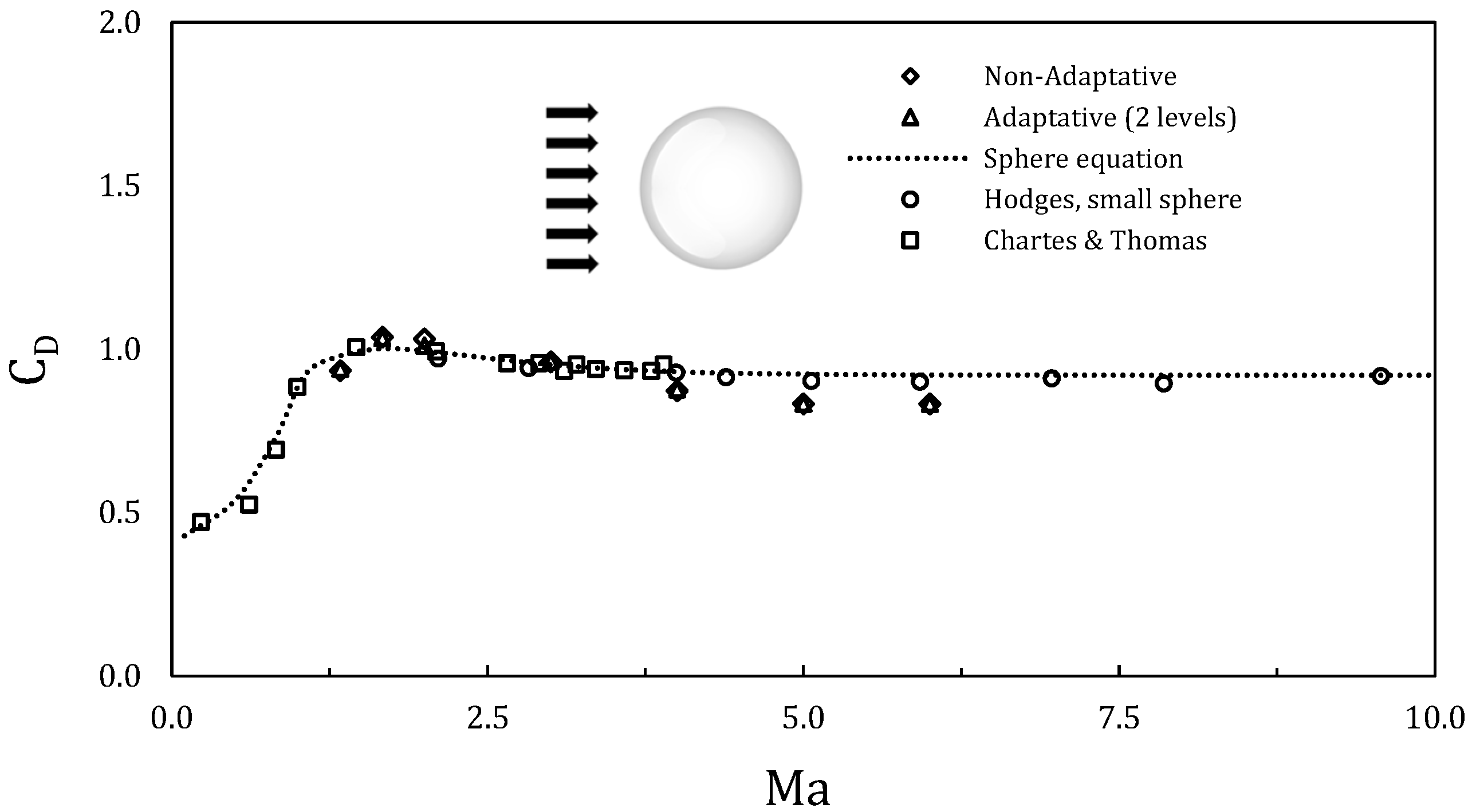
The validation is performed with a smooth sphere for different Mach numbers ranging from 0.9 to 6.0. The variances between results obtained with the fine and coarse grids are less than 5%, but with relative errors slightly higher than 10% regard to the experimental and numerical results of drag coefficient of a sphere. Adaptative mesh of 2 levels shows a slightly better performance in compare with other mesh grids. All of them show relative errors below 9% in the whole range of Mach number. However, adaptative mesh time simulation is considerably higher than fine refinement, therefore this one was selected for validation and dataset creation, see
Figure 2. Overall, results show good agreement with the experimental data.
Figure 1.
Mach number vs. aerodynamics drag coefficient. Adaptative and non-adaptative meshes showed very similar results. In comparison with experimental data, both simulations.
Figure 1.
Mach number vs. aerodynamics drag coefficient. Adaptative and non-adaptative meshes showed very similar results. In comparison with experimental data, both simulations.
2.2. Spike Blunt Body Protoype
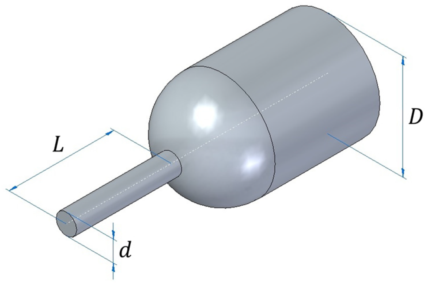
The proposed model analysed is a flat-face spike blunt body with a diameter (
d) and a length (
L) and a blunt body diameter (
D) of 1 inch, see
Figure 2. These parameters are treated as dimensionless, as shown in the next section.
Figure 2.
Blunt body scheme with main dimensions.
Figure 2.
Blunt body scheme with main dimensions.
Once the numerical model has been validated and the geometry of interest is defined, it is possible to perform the simulations that supplies dataset of Machine Learning algorithm.
2.3. Dataset
As mentioned earlier, a reliable and complete dataset is essential to provide information to the ML Algorithm. The predictions were developed over a wide range of Mach numbers, aspect ratios, and Reynolds. The dataset needed to feed selected machine learning model was generated through sets of simulations based on
Table 1 using SolidWorks Flow simulation. Overall, 239 simulations were considered. The dataset used in this work is built with simulation results of geometry dimensions described previously. Variables considered are force over x direction, velocity, density, viscosity, speed of sound, spike diameter, and spike length.
Input variables are converted into dimensionless parameters decreasing the number of input variables in consequence dataset size. The dataset includes drag coefficient
Cd, Reynolds number
Re, Mach number
Ma,
d/D dimensionless spike diameter ratio and
L/D dimensionless spike length ratio.
The predictions were developed over a wide range of Mach number, Reynolds number, and aspect ratios. The spike diameter ratio ranged from 0.06 to 0.18 times blunt body diameter at intervals of 0.02, while spike length ratio ranged from 0.15 to 2.15 times blunt body diameter at intervals of 0.5. Subsequently, these relations are named aspect ratios. The dataset needed to feed selected machine learning model was generated through sets of simulations based on
Table 1 using SolidWorks Flow simulation. Overall, 239 simulations were considered.
Table 2.
Each aspect ratio of diameter (d/D) and length (L/D) is tested for each Ma number.
Table 2.
Each aspect ratio of diameter (d/D) and length (L/D) is tested for each Ma number.
| Ma |
Re |
| 1.2 |
4.7 × 10⁵
|
| 1.6 |
6.2 × 10⁵
|
| 2.0 |
7.8 × 10⁵
|
| 2.4 |
9.3 × 10⁵
|
| 2.8 |
1.0 × 10⁶
|
| 3.2 |
1.2 × 10⁶
|
Some of the postprocessed data obtained from the numerical simulations are presented in the results section. This is because one of the objectives of the simulations is to obtain the value of the drag coefficient for dataset of the algorithm, but it is also to capture the physical phenomenon of shock waves as part of the validation. Results are presented in section 3.
2.4. k-NN Model
K-Nearest neighbours is one of the most versatile, intuitive, easy to understand and implement, making accesible for practioners and reserchers. This is supervised model, which based its effectiveness in the power of proximity. K-Nearest neighbours do not make any assumptions about data distribution, which make it suitable for wide range of datasets, even those with non-linear or complex relationships among variables.
Unlike some other machine learning algorithms that require a large amount of data to work properly, k-NN regression can still produce proper results with small datasets, as long as the data is representative of the problem space. k-NN is suitable for recomentation systems, customer segmentation, medical diagnosis and quality control.
k-NN present some disadvantages, one of them is that it uses the entire dataset to train “each point” and therefore requires the use of a lot of memory and processing resources (CPU). For these reasons k-NN tends to work better on small datasets and without a huge number of features (columns). k-NN also presents high sensitivity to irrelevant features, due to they can hace large impact on the distance metric selected to identify the nearest neighbours, than can result in a poor performace if the features are not processed properly.
Considering information previously mentioned, k-NN as regression has been selected as a method to predict drag performace.
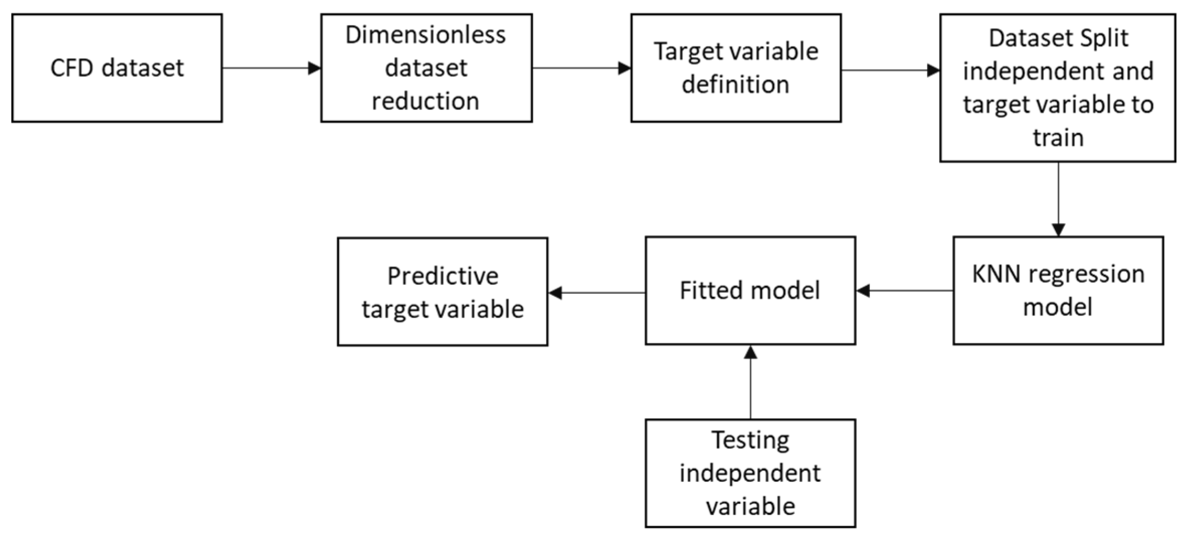
Figure 3.
k-NN and CFD implementation.
Figure 3.
k-NN and CFD implementation.
The k-NN is calibrated by two parameters, "k" and "distance metric", where "k" represents the number of neighbours considered and the "distance metric" measures the similarity between data points. By considering the k nearest neighbours and using a distance metric to measure similarity, the k-NN algorithm in regression can make predictions for new datapoints based on the patterns observed in the training data. The Euclidian distance is calculated as:
The accuracy of predicted values is compared with simulations results using determination coefficient (R
2) values and the selection of "k" neighbours is based of model accuracy:
For experiments, 70% of the dataset is considered for training while 30% is used for testing. Several k close neighbours are used, and prediction is computed based on Euclidean distance.
3. Results and Discussion
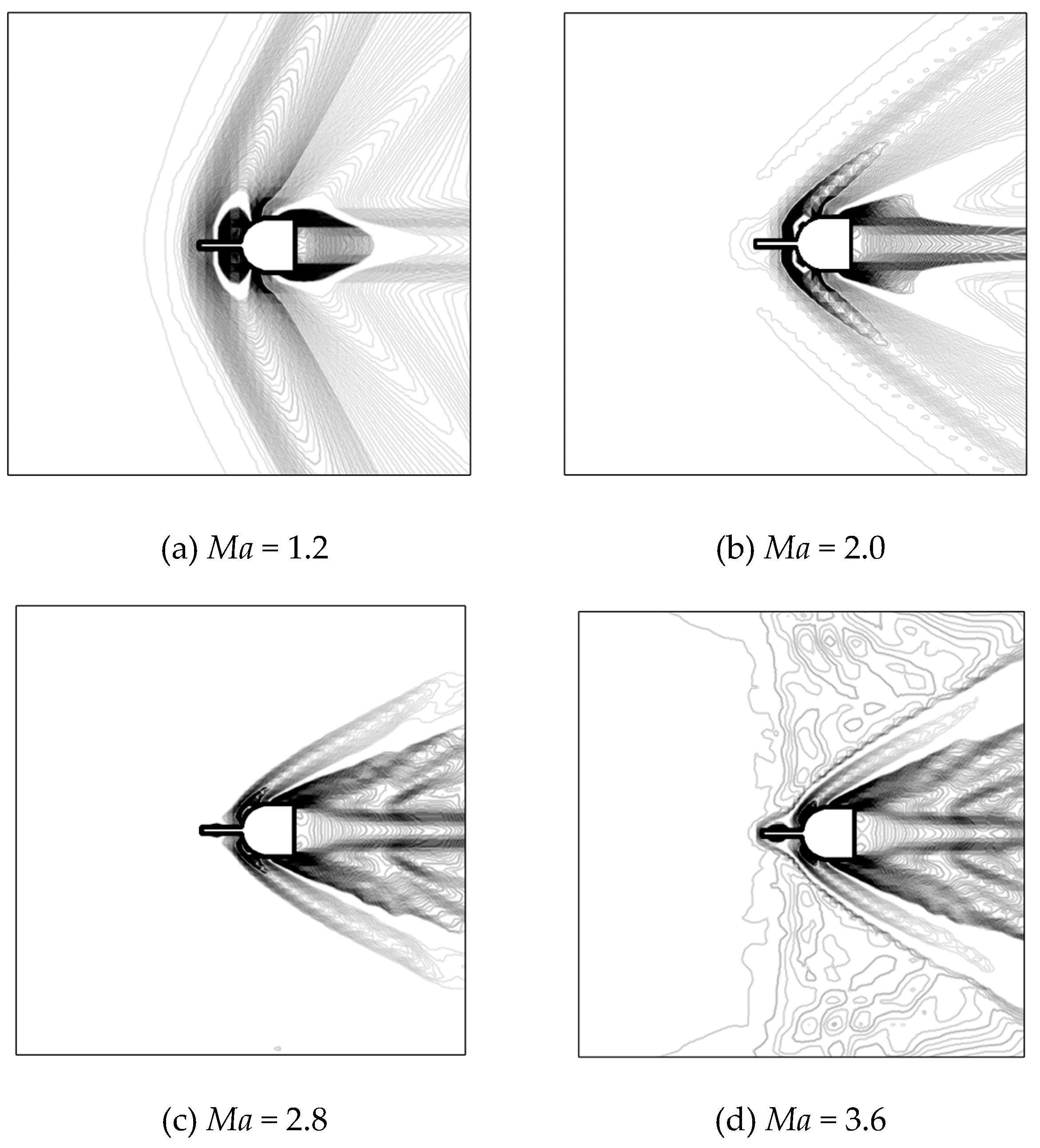
In order to show simulation performance and verify that simulations are capturing the phenomenon,
Figure 4 presents the shock wave formation system by using the numerical Schlieren technique for four different Mach (Ma) numbers with the same geometrical relationship. This is done by visualizing the contours of absolute density gradient (|∇ρ|) [
35]. The images presented expose the overall flow behavior, demonstrating how the strong oblique shock wave found in blunt bodies is broken down into a group of lower-intensity shock waves. In
Figure 4 (b), (c) and (d), the characteristic recirculation and reattachment zones are observed, along with the reattachment shock wave seen in spiked blunt bodies under high Mach conditions [
36]. However, for the Ma = 1.2, it is possible to see that the bow shock wave only is moved upstream in front of the spike, reason why a significant reduction in drag is not achieved under transonic flow conditions. Therefore, numerical software is capable of adequately reproducing most of the physics involved in spike blunt bodies subjected to transonic and supersonic flow conditions. Thus, the capture of these flow characteristics, make a well suited drag prediction by using the CFD Tool.
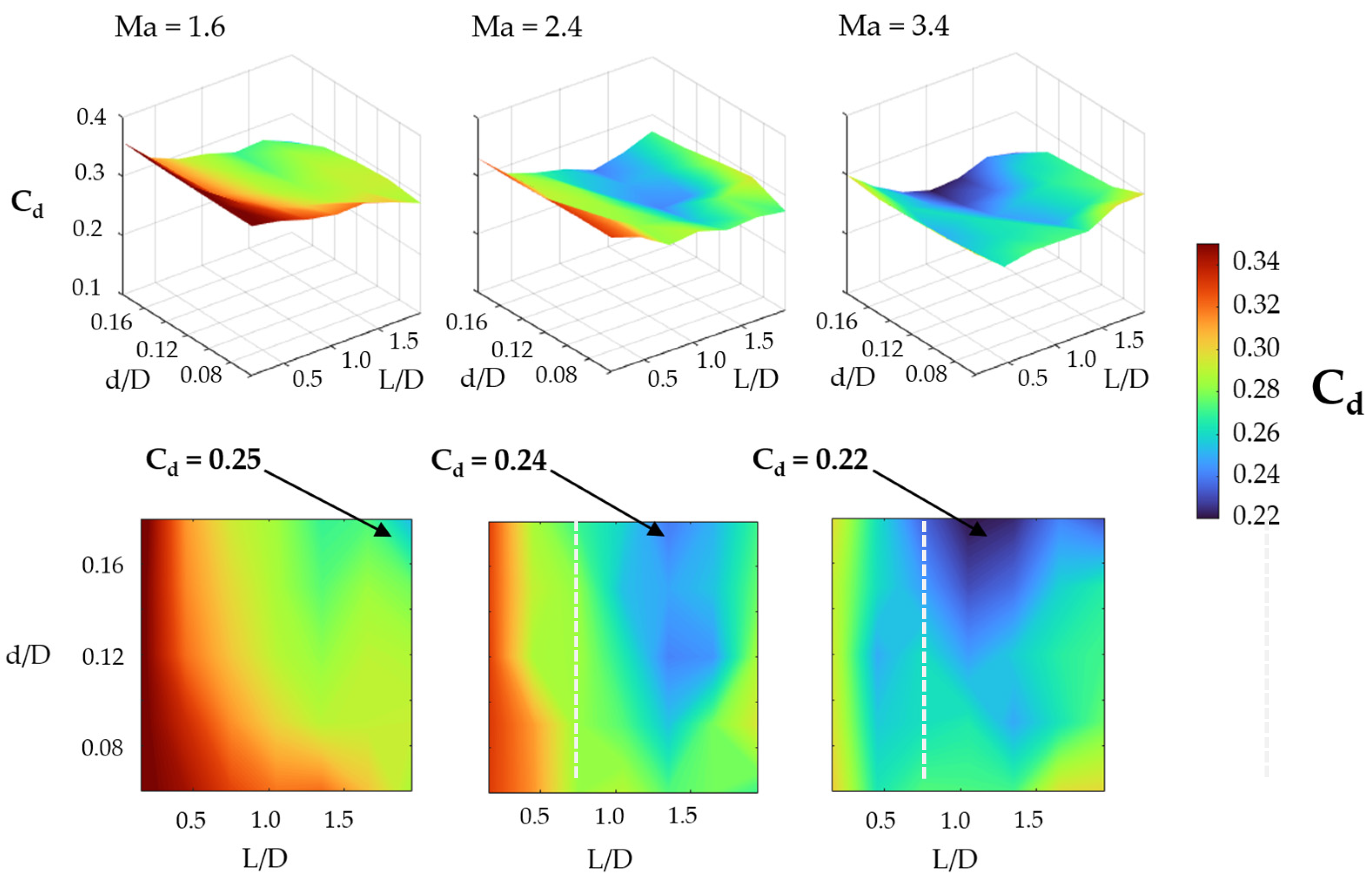
On the other hand, to show the effectiveness of the spike on the blunt body, and the quality and relevance of the dataset used by the k-NN model numerical simulations results of drag coefficient are presented. The effectiveness of the spike is reflected in the aerodynamic drag reduction. Surface plots of C
d are shown in the upper part of
Figure 5.
The surface in the upper part of
Figure 5 might seem like each other, regardless of the aspect ratio of the spike (d/D or L/D), but the surfaces show lower values as the
Ma increases. A first increase in the
Ma (1.6→2.4) reduces the average drag coefficient (
Cd,average) by 5.1%, and a second increase (2.4→3.2) reduces the coefficient by another 7.5%, as shown in
Table 3.
As shown in the lower part of
Figure 5, the general tendency of the C
d is to reduce its value as the spike length increases, which is consistent with several works [
10,
11,
12,
13,
14,
15,
16]. Within our range of spike length ratios values above 1 time the blunt body diameter presents the best performance. For short spike length ratios (lower than 0.5), this extruded geometry from the blunt body is ineffective to reduce the drag force. The primary shock wave formed by the spike does not affect the secondary shock wave of the blunt body and it occurs at any spike diameter ratio.
Until this point, the study has provided insights which explain drag coefficient performance for a flat spike blunt body with respect to Mach number, Reynolds number, dimensionless spike diameter ratio and dimensionless spike length ratio. As mentioned in previous sections, to identify that phenomenon was captured correctly, Schlieren technique (
Figure 4) is used to identify shockwave formations and drag reduction (
Figure 5) is observed. All simulations were performed at the same computer (Dell precision 7530 wkst intel core xeon e-2176m / memory 16 gb). In average simulation takes 10 minutes per case. Python sklearn library is used to implement k-NN model. To train it 70% of total dataset was used for training while 30% for testing. The k-NN model was tested for different neighbours to identify proper numbers.
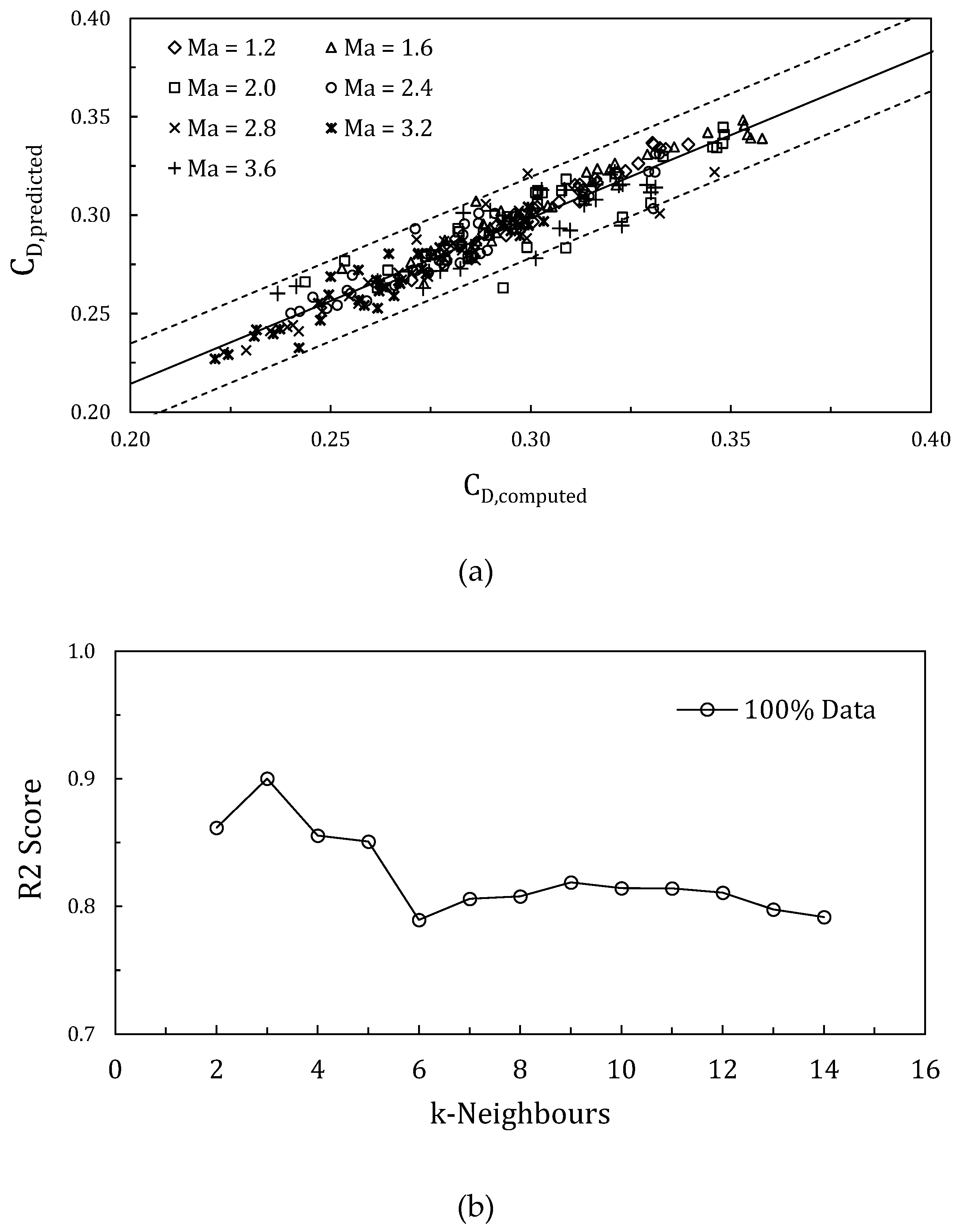
Figure 6 presents results of k-NN model and test error for different neighbours’ numbers.
Figure 6 (a) shows a comparison of tested data against model predicted values. It can be observed that for drag coefficient prediction, 209 out of 239 data points are lying within the ±5% error range, around 87% of total data. Which is consistent with previous studies that combined computational fluid dynamics and k-NN model [
37].
Different k neighbours were tested and recorded.
Figure 6 (b) shows that k = 3 is predicting the highest accuracy for drag reduction, R2 value for drag reduction is 0.90. The k-NN regression algorithm demonstrates impressive accuracy, making it an excellent tool for engineers to predict outputs without the need for computationally solving the drag reduction system.
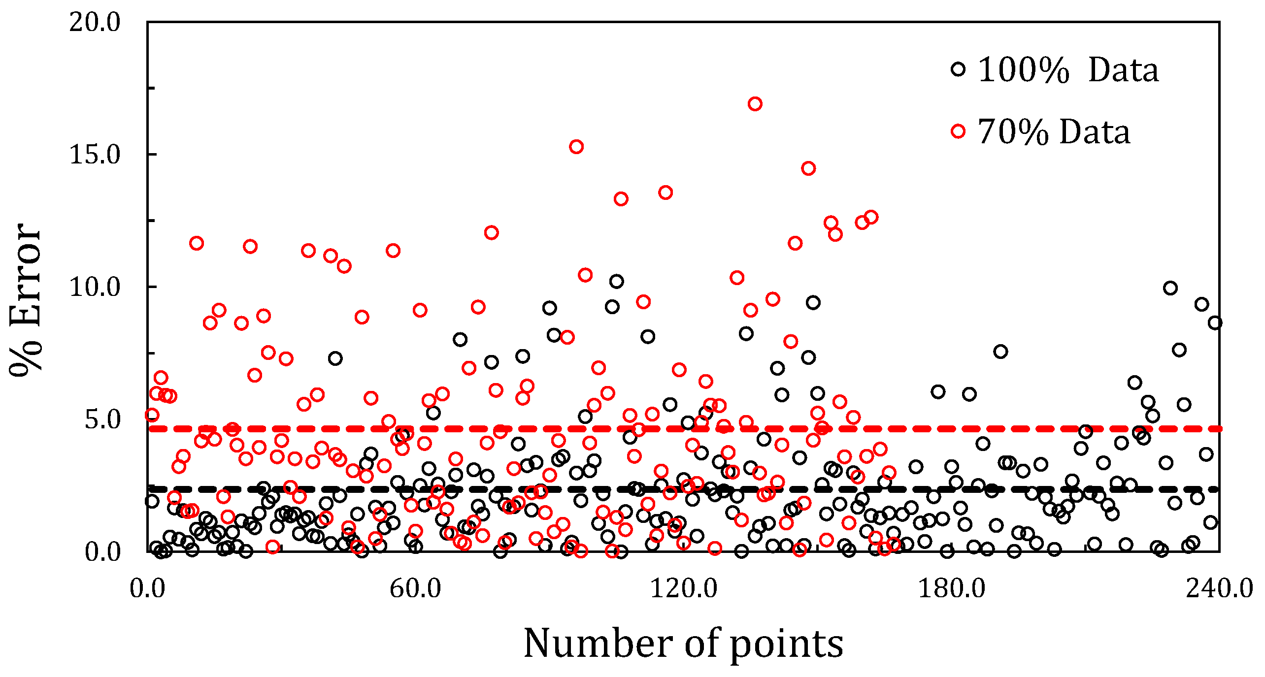
Figure 7 shows the error difference between
computed and
predicted for 100% of data simulation and random sample of 70% of dataset. In this case is possible to observe that despite of accuracy decreases for 70% sample, there is still a significant amount of data lying in 10% of error.
Due time is critical for CFD practitioners and dataset creation can be substantial time consuming a set of similar tests were performed reducing the amount of data in 70% and 50% generating aleatory datasets samples respectively, to test average amount of data predicted lying ±10% of error.
Table 4 presents average errors considering different samples.
According to
Table 4, datasets with 70% of total dataset present that in average 89% of data lying in an error under 10%, while dataset 50% of total dataset did it at approximately 85%. This result presents similar performances as work presented by Krishnayatra [
37], where almost same amount of data presents similar results.
4. Conclusions
This study provides insights over the physical variations overall drag coefficient reduction of a flat spike blunt, with respect to force over x direction, velocity, density, viscosity, speed of sound, spike diameter, and spike length. Parameters were reduced to their non-dimensional form. Therefore, Mach number Ma variates from 1.2 to 3.6, d/D dimensionless spike diameter ratio and L/D spike length ratio ranged from 0.06 to 0.18 and from 0.15 to 2.15 times blunt body diameter, respectively.
According to the results presented in this research, solid works flow simulation with selected mesh have been able to capture shock wave performance. Observing the recirculation and reattachment zone at supersonic flow conditions Ma = 2.0, 2.8 and 3.6. While for Ma = 1.2, the bow shock wave only is moved upstream in front of the spike, reason why a significant reduction in drag is not achieved. On the other hand, it is observed that as soon as Ma number increases, drag coefficient reduces between 5% to 7.5 %.
Despite machine learning emerging as a valuable tool, its implementation can be privative when there is a lack computational sources or of expertise in machine learning. In this sense, k-NN has shown that it can be a suitable model, not just for accuracy or its easy implementation, the use of a small data set makes it appropriate to create in a small period of time enough data to predict performance. According to the methodology used, the reduction of data through dimensionless parameters in conjunction with k-NN model have presented an accuracy close to 95% and even reducing data set, good performance can be obtained.
Future research will focus on applied current methodology for parameters such as heat transfer as well as other physical characteristics like angle attack or shapes.
Author Contributions
Conceptualization, J.A.S.M. and J.R.C.; methodology, J.A.S.M.; software, J.A.S.M.; validation, J.A.S.M., C.L.C. and J.R.C.; formal analysis, J.A.S.M., C.L.C. and J.R.C.; investigation, J.A.S.M., C.L.C. and J.R.C.; resources, J.A.S.M.; data curation, J.A.S.M.; writing—original draft preparation, J.A.S.M., C.L.C. and J.R.C.; writing—review and editing, J.A.S.M., C.L.C. and J.R.C.; visualization, C.L.C.; supervision, J.A.S.M.; project administration, J.A.S.M.; funding acquisition, J.A.S.M.
Funding
The APC was funded by Tecnologico de Monterrey, Vicerrectory of Research and Technology Transfer.
Data Availability Statement
Dataset used for prediction.
| d/D |
L/D |
Cd comp Ma = 1.2 |
Cd comp Ma = 1.6 |
Cd comp Ma = 2.0 |
Cd comp Ma = 2.4 |
Cd comp Ma = 2.8 |
Cd comp Ma = 3.2 |
Cd comp Ma = 3.6 |
| 0.06 |
0.15 |
0.3304 |
0.353 |
0.348 |
0.3312 |
0.3459 |
0.3032 |
0.3229 |
| 0.06 |
0.45 |
0.3268 |
0.3442 |
0.333 |
0.3145 |
0.2887 |
0.2645 |
0.321 |
| 0.06 |
0.75 |
0.3217 |
0.3291 |
0.3088 |
0.2834 |
0.2828 |
0.2738 |
0.322 |
| 0.06 |
1.05 |
0.3165 |
0.3197 |
0.3133 |
0.2891 |
0.2749 |
0.2728 |
0.3027 |
| 0.06 |
1.35 |
0.3117 |
0.3213 |
0.3016 |
0.274 |
0.28 |
0.2719 |
0.3139 |
| 0.06 |
1.65 |
0.3122 |
0.3053 |
0.3028 |
0.2783 |
0.299 |
0.2973 |
0.3084 |
| 0.06 |
1.95 |
0.2971 |
0.2863 |
0.33 |
0.2711 |
0.2861 |
0.2993 |
0.3162 |
| 0.09 |
0.15 |
0.3307 |
0.3533 |
0.3483 |
0.3321 |
0.2992 |
0.2976 |
0.329 |
| 0.09 |
0.45 |
0.3236 |
0.3358 |
0.3213 |
0.313 |
0.3322 |
0.2569 |
0.3198 |
| 0.09 |
0.75 |
0.313 |
0.3152 |
0.2941 |
0.283 |
0.2714 |
0.2621 |
0.3133 |
| 0.09 |
1.05 |
0.3016 |
0.3007 |
0.2827 |
0.2744 |
0.2593 |
0.2658 |
0.2831 |
| 0.09 |
1.35 |
0.298 |
0.2898 |
0.2752 |
0.2554 |
0.267 |
0.2495 |
0.3072 |
| 0.09 |
1.65 |
0.3005 |
0.2913 |
0.2818 |
0.279 |
0.2862 |
0.2638 |
0.2898 |
| 0.09 |
1.95 |
0.2915 |
0.2925 |
0.3229 |
0.2961 |
0.2783 |
0.2772 |
0.3098 |
| 0.12 |
0.15 |
0.3322 |
0.3541 |
0.3479 |
0.331 |
0.297 |
0.295 |
0.3311 |
| 0.12 |
0.45 |
0.3161 |
0.321 |
0.3077 |
0.287 |
0.2791 |
0.25 |
0.3162 |
| 0.12 |
0.75 |
0.307 |
0.3042 |
0.2821 |
0.285 |
0.2632 |
0.2617 |
0.2996 |
| 0.12 |
1.05 |
0.2969 |
0.2895 |
0.2851 |
0.266 |
0.2478 |
0.2469 |
0.2824 |
| 0.12 |
1.35 |
0.2883 |
0.2828 |
0.2683 |
0.2422 |
0.2546 |
0.257 |
0.2367 |
| 0.12 |
1.65 |
0.2861 |
0.2902 |
0.2535 |
0.2455 |
0.2743 |
0.2673 |
0.2617 |
| 0.12 |
1.95 |
0.2821 |
0.2881 |
0.3087 |
0.2874 |
0.2776 |
0.2718 |
0.3012 |
| 0.15 |
0.15 |
0.3337 |
0.3549 |
0.3464 |
0.3294 |
0.2938 |
0.2927 |
0.33 |
| 0.15 |
0.45 |
0.3122 |
0.3166 |
0.3017 |
0.291 |
0.2703 |
0.2614 |
0.3122 |
| 0.15 |
0.75 |
0.3007 |
0.2995 |
0.2896 |
0.2823 |
0.2478 |
0.2474 |
0.2964 |
| 0.15 |
1.05 |
0.2975 |
0.2864 |
0.2785 |
0.2541 |
0.2349 |
0.2309 |
0.2774 |
| 0.15 |
1.35 |
0.2813 |
0.275 |
0.2643 |
0.249 |
0.2406 |
0.2373 |
0.2414 |
| 0.15 |
1.65 |
0.2854 |
0.2843 |
0.2737 |
0.255 |
0.2569 |
0.2584 |
0.2731 |
| 0.15 |
1.95 |
0.2734 |
0.2785 |
0.299 |
0.2771 |
0.2678 |
0.2669 |
0.2746 |
| 0.18 |
0.15 |
0.3393 |
0.3578 |
0.3454 |
0.3306 |
0.2926 |
0.2994 |
0.3227 |
| 0.18 |
0.45 |
0.311 |
0.3139 |
0.3012 |
0.2869 |
0.2671 |
0.2623 |
|
| 0.18 |
0.75 |
0.2958 |
0.2941 |
0.2881 |
0.2705 |
0.2392 |
0.2356 |
|
| 0.18 |
1.05 |
0.2938 |
0.2851 |
0.2843 |
0.259 |
0.2233 |
0.2211 |
|
| 0.18 |
1.35 |
0.2798 |
0.27 |
0.2617 |
0.24 |
0.2289 |
0.2244 |
|
| 0.18 |
1.65 |
0.2779 |
0.2733 |
0.2436 |
0.2516 |
0.242 |
0.2421 |
|
| 0.18 |
1.95 |
0.2702 |
0.2528 |
0.2931 |
0.2714 |
0.2522 |
0.2314 |
|
Conflicts of Interest
The authors declare no conflict of interest.
References
- Anderson, J.D. Fundamentals of Aerodynamics, 6th ed.; McGraw-Hill: New York, USA, 2017. [Google Scholar]
- Rashid, S.; Nawaz, F.; Maqsood, A.; Salamat, S.; Riaz, R. Review of Wave Drag Reduction Techniques: Advances in Active, Passive, and Hybrid Flow Control. Proc. Inst. Mech. Eng. G: J. Aerosp. Eng. 2022, 236, 2851–2884. [Google Scholar] [CrossRef]
- Bertin, J.J.; Cummings, R.M. Fifty Yxears of Hypersonics: Where We’ve Been, Where We’re Going. Prog. Aerosp. Sci. 2003, 39, 511–536. [Google Scholar] [CrossRef]
- Bertin, J.J.; Bouslog, S.A.; Wang, K.-C.; Campbell, C.H. Recent Aerothermodynamic Flight Measurements during Shuttle Orbiter Re-Entry. J. Spacecr. Rockets 1996, 33, 457–462. [Google Scholar] [CrossRef]
- Schneider, S.P. Flight Data for Boundary-Layer Transition at Hypersonic and Supersonic Speeds. J. Spacecr. Rockets 1999, 36, 8–20. [Google Scholar] [CrossRef]
- Hollis, B.R.; Borrelli, S. Aerothermodynamics of Blunt Body Entry Vehicles. Prog. Aerosp. Sci. 2012, 48–49, 42–56. [Google Scholar] [CrossRef]
- Huang, W.; Chen, Z.; Yan, L.; Yan, B.; Du, Z. Drag and Heat Flux Reduction Mechanism Induced by the Spike and Its Combinations in Supersonic Flows: A Review. Prog. Aerosp. Sci. 2019, 105, 31–39. [Google Scholar] [CrossRef]
- Guenther, R.A.; Reding, J.P. Fluctuating Pressure Environment of a Drag Reduction Spike. J. Spacecr. Rockets 1977, 14, 705–710. [Google Scholar] [CrossRef]
- Ahmed, M.Y.M.; Qin, N. Recent Advances in the Aerothermodynamics of Spiked Hypersonic Vehicles. Prog. Aerosp. Sci. 2011, 47, 425–449. [Google Scholar] [CrossRef]
- Esfeh, M.K.; Tajalli, S.M.; Liu, P. Evaluation of Aerospike for Drag Reduction on a Blunt Nose Using Experimental and Numerical Modeling. Acta Astronaut. 2019, 160, 656–671. [Google Scholar] [CrossRef]
- Tekure, V.; Pophali, P.S.; Venkatasubbaiah, K. Numerical Investigation of Aerospike Semi-Cone Angle and a Small Bump on the Spike Stem in Reducing the Aerodynamic Drag and Heating of Spiked Blunt-Body: New Correlations for Drag and Surface Temperature. Phys. Fluids 2021, 33, 116108. [Google Scholar] [CrossRef]
- Kalimuthu, R.; Mehta, R.C.; Rathakrishnan, E. Investigation of Aerodynamic Coefficients at Mach 6 over Conical, Hemispherical and Flat-Face Spiked Body. Aeronaut. J. 2017, 121, 1711–1732. [Google Scholar] [CrossRef]
- Li, Z.; Sun, C.; Xia, X.; Li, X. Numerical Simulation of Aerodynamic Heating over Solid Blunt Configuration with Porous Spike. J. Aerosp. Eng. 2018, 31, 04018083. [Google Scholar] [CrossRef]
- Asif, M.; Zahir, S.; Kamran, N.; Khan, M. Computational Investigations Aerodynamic Forces at Supersonic / Hypersonic Flow Past a Blunt Body with Various Forward Facing Spikes. In Proceedings of the 22nd Applied Aerodynamics Conference and Exhibit; Guidance, Navigation, and Control and Co-located Conferences; AIAA, 2004. [Google Scholar]
- Xue, Y.; Wang, L.; Fu, S. Drag Reduction and Aerodynamic Shape Optimization for Spike-Tipped Supersonic Blunt Nose. J. Spacecr. Rockets 2018, 55, 552–560. [Google Scholar] [CrossRef]
- Hamza, M.; Khan, S.B.; Maqsood, A. Geometric Optimization of Blunt Bodies with Aerodisk and Opposing Jet for Wave Drag and Heat Reduction. Aerospace 2022, 9, 800. [Google Scholar] [CrossRef]
- Brunton, S.L.; Noack, B.R.; Koumoutsakos, P. Machine Learning for Fluid Mechanics. Annu. Rev. Fluid Mech. 2020, 52, 477–508. [Google Scholar] [CrossRef]
- Vinuesa, R.; Brunton, S.L. Enhancing Computational Fluid Dynamics with Machine Learning. Nat. Comput. Sci. 2022, 2, 358–366. [Google Scholar] [CrossRef]
- Kou, J.; Zhang, W. Data-Driven Modeling for Unsteady Aerodynamics and Aeroelasticity. Prog. Aerosp. Sci. 2021, 125, 100725. [Google Scholar] [CrossRef]
- Li, J.; Du, X.; Martins, J.R.R.A. Machine Learning in Aerodynamic Shape Optimization. Prog. Aerosp. Sci. 2022, 134, 100849. [Google Scholar] [CrossRef]
- Bianco, M.J.; Gerstoft, P.; Traer, J.; Ozanich, E.; Roch, M.A.; Gannot, S.; Deledalle, C.-A. Machine Learning in Acoustics: Theory and Applications. J. Acoust. Soc. Am. 2019, 146, 3590–3628. [Google Scholar] [CrossRef]
- Kužnar, D.; Možina, M.; Giordanino, M.; Bratko, I. Improving Vehicle Aeroacoustics Using Machine Learning. Eng. Appl. Artif. Intell. 2012, 25, 1053–1061. [Google Scholar] [CrossRef]
- Alguacil, A.; Bauerheim, M.; Jacob, M.C.; Moreau, S. Predicting the Propagation of Acoustic Waves Using Deep Convolutional Neural Networks. J. Sound Vib. 2021, 512, 116285. [Google Scholar] [CrossRef]
- Salehi, H.; Das, S.; Chakrabartty, S.; Biswas, S.; Burgueño, R. Damage Identification in Aircraft Structures with Self-Powered Sensing Technology: A Machine Learning Approach. Struct. Contr. Health Monit. 2018, 25, e2262. [Google Scholar] [CrossRef]
- de Jong, M.; Chen, W.; Notestine, R.; Persson, K.; Ceder, G.; Jain, A.; Asta, M.; Gamst, A. A Statistical Learning Framework for Materials Science: Application to Elastic Moduli of k-Nary Inorganic Polycrystalline Compounds. Sci. Rep. 2016, 6, 34256. [Google Scholar] [CrossRef] [PubMed]
- Linse, D.J.; Stengel, R.F. Identification of Aerodynamic Coefficients Using Computational Neural Networks. J. Guid. Control Dyn. 1993, 16, 1018–1025. [Google Scholar] [CrossRef]
- Suresh, S.; Omkar, S.N.; Mani, V.; Guru Prakash, T.N. Lift Coefficient Prediction at High Angle of Attack Using Recurrent Neural Network. Aerosp. Sci. Technol. 2003, 7, 595–602. [Google Scholar] [CrossRef]
- Secco, N.R.; De Mattos, B.S. Artificial Neural Networks to Predict Aerodynamic Coefficients of Transport Airplanes. Aircr. Eng. Aerosp. Tech. 2017, 89, 211–230. [Google Scholar] [CrossRef]
- Ghoreyshi, M.; Jirásek, A.; Cummings, R.M. Computational Approximation of Nonlinear Unsteady Aerodynamics Using an Aerodynamic Model Hierarchy. Aerosp. Sci. Technol. 2013, 28, 133–144. [Google Scholar] [CrossRef]
- Wang, X.; Kou, J.; Zhang, W. Unsteady Aerodynamic Modeling Based on Fuzzy Scalar Radial Basis Function Neural Networks. Proc. Inst. Mech. Eng. G: J. Aerosp. Eng. 2019, 233, 5107–5121. [Google Scholar] [CrossRef]
- Hou, W.; Darakananda, D.; Eldredge, J.D. Machine-Learning-Based Detection of Aerodynamic Disturbances Using Surface Pressure Measurements. AIAA J. 2019, 57, 5079–5093. [Google Scholar] [CrossRef]
- Taunk, K.; De, S.; Verma, S.; Swetapadma, A. A Brief Review of Nearest Neighbor Algorithm for Learning and Classification. In Proceedings of the 2019 International Conference on Intelligent Computing and Control Systems (ICCS); 2019; pp. 1255–1260. [Google Scholar]
- Hodges, A.J. The Drag Coefficient of Very High Velocity Spheres. J Aeronaut Sci. 1957, 24, 755–758. [Google Scholar] [CrossRef]
- Charters, A.C.; Thomas, R.N. The Aerodynamic Performance of Small Spheres from Subsonic to High Supersonic Velocities. J Aeronaut Sci. 1945, 12, 468–476. [Google Scholar] [CrossRef]
- Ahmad, H.; Hasan, N.; Sanghi, S. On the Influence of Co-Flow on the Shocks and Vortex Rings in the Starting Phases of under-Expanded Jets. Phys. Fluids 2022, 34, 076117. [Google Scholar] [CrossRef]
- Tahani, M.; Karimi, M.S.; Motlagh, A.M.; Mirmahdian, S. Numerical Investigation of Drag and Heat Reduction in Hypersonic Spiked Blunt Bodies. Heat Mass Transf. 2013, 49, 1369–1384. [Google Scholar] [CrossRef]
- Krishnayatra, G.; Tokas, S.; Kumar, R. Numerical Heat Transfer Analysis & Predicting Thermal Performance of Fins for a Novel Heat Exchanger Using Machine Learning. Case Stud. Therm. Eng. 2020, 21, 100706. [Google Scholar] [CrossRef]
|
Disclaimer/Publisher’s Note: The statements, opinions and data contained in all publications are solely those of the individual author(s) and contributor(s) and not of MDPI and/or the editor(s). MDPI and/or the editor(s) disclaim responsibility for any injury to people or property resulting from any ideas, methods, instructions or products referred to in the content. |
© 2024 by the authors. Licensee MDPI, Basel, Switzerland. This article is an open access article distributed under the terms and conditions of the Creative Commons Attribution (CC BY) license (http://creativecommons.org/licenses/by/4.0/).
