Preprint
Article

Forecasting of Standardized Precipitation Index using Hybrid Models: A Case Study of Cape Town, South Africa

Altmetrics

Downloads

118

Views

47

Comments

0

A peer-reviewed article of this preprint also exists.

Submitted:

22 July 2024

Posted:

24 July 2024

You are already at the latest version

Alerts
Abstract
Droughts have negative impacts on agricultural productivity and economic growth. Effective monitoring and accurate forecasting of drought occurrences and trends are crucial for minimizing drought losses and mitigating their spatial and temporal effects. In this study, trend dynamics in monthly total rainfall time series measured at Cape Town International Airport were analyzed using Mann-Kendall (MK) test, Modified Mann-Kendall (MMK) and innovative trend analysis (ITA) were examined. Additionally, we utilized hybrid prediction method that combined the model with the complementary ensemble empirical mode decomposition with adaptive noise (CEEMDAN) technique, the autoregressive integrated moving average (ARIMA) model, the long short-term memory (LSTM) network (i.e. CEEMDAN-ARIMA-LSTM) to forecast SPI values of 6-, 9-, and 12-months using rainfall data between 1995 and 2020 from Cape Town International Airport meteorological rainfall stations. The results demonstrate the following essential points: (1) The trend analysis results of the total monthly rainfall values indicate a significant decreasing trend with the negative z-score (MK= -3.7541 and MMK= - 4.0773). ITA also indicated a significant downwards trend of rainfall in the study area. (2) As the forecasting horizon increases, the prediction accuracy of the models and CEEMDAN-combined models gradually improves, reaching their optimum performance at the 12-month horizon. (3) CEEMDAN efficiently stabilizes time-series data, resulting in greater prediction accuracy in the hybrid model compared to individual models at all timescales. (4) The RMSE and R2 values for the hybrid CEEMDAN-ARIMA-LSTM model at a 12-month forecasting horizon are 0.042 and 0.995, demonstrating the applicability of this hybrid approach for drought forecasting.
Keywords: 
Subject: Environmental and Earth Sciences  -   Water Science and Technology

1. Introduction

Drought is a gradual and pernicious natural catastrophic event with global socioeconomic and environmental consequences. This is a highly perilous climate-related catastrophe that has a substantial effect on both the environment and human existence [1]. Droughts have a profound effect on municipal water supplies, which is one of their most important effects. These supplies refer to the purified water distributed to households and businesses, which is crucial for human consumption, cleanliness, and numerous critical services on a global scale [2]. Municipal water sources are given priority during drought and water constraint due to their significant sociological and economic relevance. This prioritization entails reallocating available water resources, frequently diverting them away from other sectors, especially agriculture, to ensure the uninterrupted supply of water to urban areas and their residents [3]. During extremely severe drought circumstances, the water sources that urban water systems depend on can be exhausted, leading to a scarcity of municipal water for consumers.
In 2018, Cape Town and another part of the country faced acute water shortages as a result of drought. These occurrences and growing concerns about water scarcity in urban areas are the result of several factors, including rising demand for water due to population growth, unpredictable weather patterns, the effects of climate change, and, in some cases, insufficient planning and management of water infrastructure [4,5]. In addition, the exploitation of surface water and groundwater resources, which have historically supplied water for human sustenance and agriculture, has reached unsustainable levels in several countries, resulting in negative environmental consequences [6]. The excessive use of these natural water resources has led to the contamination of certain water bodies, such as the salinization of over-exploited aquifers or the inability to dilute and assimilate wastewater discharges, rendering the water supplies unsuitable for human consumption [7]. To maintain a secure and stable water supply in the present and the future, it is essential to recognize that the development of resilient water systems is an imperative necessity [8]. In disaster management, the application of time series forecasting methodologies can serve as an early warning system.
The significance of addressing drought-related issues has increased as time series analysis continues to advance. Prediction of drought requires the management of complex, often nonstationary, nonlinear precipitation data, and SPI time series. Rarely do we encounter simple and stable time series in practice. Consequently, it is of the utmost importance to identify an efficient method for addressing the complexities of nonlinear and nonstationary time series and for making accurate forecasts. Nonetheless, due to the complexities of evaluating time series precision, devising suitable forecasting models remains a formidable challenge [9].
In recent years, numerous models, such as the Autoregressive Integrated Moving Average (ARIMA) model, have been utilized for drought forecasting due to its their adaptability and greater information on time-related changes [10]. However, they have difficulty accurately predicting nonlinear data [11]. As machine learning has evolved, the Long Short-Term Memory (LSTM) network has emerged as a solution to resolve long-term dependencies, especially in sequences with extended intervals and delays [12]. The LSTM model has shown promising results when applied to the prediction of drought time series and related domains [13,14,15]. Nonetheless, the inherent complexity of time series frequently results in suboptimal local predictions, thereby diminishing the overall performance of forecasting [11].
To enhance time-series prediction accuracy in the face of these complexities, scholars have introduced signal decomposition techniques [16,17,18,19]. Signal decomposition efficiently removes certain characteristics from sequences, making them more stable and easier to handle. These methods streamline the initial simplify time series and enhance their predictability. Some of the methods include empirical mode decomposition (EMD), ensemble empirical mode decomposition (EEMD), complementary ensemble empirical mode decomposition (CEEMD), and complementary ensemble empirical mode decomposition with adaptive noise (CEEMDAN). CEEMD addresses both the problem of blending modes in EMD and the issue of residual white noise in EEMD. Furthermore, CEEMDAN is an enhanced iteration of CEEMD that provides enhanced adaptability in handling intricate signals with varying attributes and levels of noise. CEEMDAN is specifically intended to adaptively assess and remove noise from the signal throughout the decomposition process. This is especially advantageous when the input signal is contaminated by noise, as it enhances the integrity of the recovered components. Xu et al. [20] utilised the CEEMD-ARIMA combined model to forecast drought in the Xinjiang Uygur Autonomous Region of China. The model outperformed the standalone ARIMA in terms of prediction accuracy across many time scales. Ding et al. [11] utilised a hybrid model combining CEEMD-LSTM to predict drought in the Xinjiang Uygur Autonomous Region of China using the standardised precipitation index. The hybrid model demonstrated superior performance compared to LSTM.
Given the non-linear and non-stationary characteristics of precipitation data, we investigate more efficient approaches for predicting time-series. Within this framework, we suggest a hybrid model called CEEMDAN-ARIMA-LSTM. This model combines the integrated empirical mode decomposition with adaptive noise (CEEMDAN), the differential integrated moving autoregressive average model (ARIMA), and the Long Short-Term Memory network (LSTM). The objective is to enhance the precision of drought prediction by capitalising on the strengths of these methods in managing intricate time series. By conducting a comparison analysis between the LSTM and ARIMA approaches, we have determined that our combined model is capable of successfully analysing and controlling the specific features of time series. This allows us to utilise both explicit and hidden data information, resulting in a substantial improvement in prediction accuracy.

2. Materials and Methods

2.1. Study Area

The data used in the study is from Cape Town as shown in Figure 1, also known as "Mother City," that which is located in the Western Cape province of South Africa, near the southernmost point of the African continent. The exact geographical coordinates are approximately 33.9249° S latitude and 18.4241° E longitude. This coastal city is located on the southwestern coast of South Africa, between the Atlantic Ocean to the west and the Hottentots-Holland Mountains to the east, creating a breathtaking natural environment that includes picturesque coastlines and Table Mountain. The unique geographical location of Cape Town has played a significant role in its history and development, contributing to the city's breathtaking natural attractiveness.

2.2. Mann-Kendall Test Statistics

Examining potential changes in the characteristics of precipitation events resulting from climate change is of utmost importance as it has significant implications for soil moisture retention, hazard assessment, and flood management. The assessment of monotonous trends in a time series of geophysical data proves consistently advantageous. The Mann-Kendall (MK) test and modified Mann-Kendall (mMK), are widely used nonparametric statistical methods, serving as an effective tool for evaluating trends in time series data. Mann first introduced this test in 1945 [21], and Kendall later refined it in 1975 [22]. The computation of the test statistic S follows the formula below.
S = j = 1 n 1 i = j + 1 n S i g n x i x j
S i g n x = f x = 1         f o r   x > 1 0         f o r   x = 1 1 ,         f o r   x < 1
Let n represent the length of the data. The data values at times i and j are denoted as x i and x j , respectively. According to Seenu and Jayakumar [23], in the Mann-Kendall test, a positive test statistic, S, suggests an increasing trend, whereas a negative test statistic indicates a decreasing trend. The variance for S is calculated using a specific mathematical formula.
V a r S = n n 1 2 n + 5 i = 1 p t i t i 1 2 t i + 5 18
The variable t i represents the number of data points in the j t h tied group, while p represents the number of the tied group in the time series. The statement indicates that the data in a time series can be compared to each other [24]. The summation procedure in the equation (3) is specifically used for linked groups in the time series. Its purpose is to minimize the impact of individual values within tied groups on the ranking statistics [25]. Assuming random and independent time series, the S statistic follows a normal distribution and can be calculated as the standardized Z statistic as follows
Z = S 1 V a r ( S )   ,           S > 0 0   ,                                 S = 0   S + 1 V a r ( S )   ,         S < 0
The Z variable follows a standard normal distribution with a variance of one and a mean of zero. The value of the S statistic is associated with the Kendall term τ , which is defined as
τ = S D
where
D = 1 2 n n 1 1 2 j = 1 p t j t j 1 1 2 1 2 n n 1 1 2
The test statistic Z is utilized to quantify the significance of trends. In fact, the null hypothesis of the MK test assumes the absence of any trend and is tested against the alternative hypothesis which assumes the presence of a trend at a specific level of significance [26,27]. Another significant outcome of the Mann-Kendall statistics is the Kendall term, which measures the correlation and indicates the strength of the relationship between any two independent variables. For serially correlated data, having a significant lag-1 autocorrelation coefficient, modified Mann-Kendall test using the Hamed and Ramachandra Rao [28] variance correlation approach was employed [29,30]. The positive and negative values of the standardize MK and MMK test statistics ( Z M K and Z M M K ) indicate increasing and decreasing trends, respectively.
The Mann-Kendall trend method can be further extended to a sequential version of the Mann-Kendall test statistic known as the Sequential Mann-Kendall (SQ-MK) test [31] with an aim to detect trends in time series [32]. The test involves comparing the original time series with its reversed counterpart to identify potential trends. The visual representation of the direct series u (   t i ) and the backward series u t i can offer valuable insights into the presence or absence of trends. The Sequential Mann-Kendall test is computed by assigning ranked values, y i , to the initial values in the analysis x 1 , x 2 , x 3 , , x n . The magnitudes of y i   (   i = 1 ,   2 ,   3 , . . . , n   ) are compared with y j   (   j = 1 ,   2 ,   3 , . . . , i 1   ) . Each comparison results in a count, denoted as n i , for the cases where y i > y j . Consequently, a statistic t i can be precisely defined as:
t i = j = 1 i n i
The distribution of test statistic t i has a mean as
E t i = i i 1 4
and variance as
V a r t i = i i 1 2 i + 5 72
Finaly, the sequential values of a reduced or standardized variable, called statistic u (   t i ) is calculated for each of the test statistic variable t i as follows:
u   t i = t i E t i V a r t i
The equation (10) provides the forward sequential statistic, u   t i , also known as the progressive statistic, which is estimated using the original time series. The backward sequential statistic, u t i , also known as the retrograde statistic, is calculated in the same way but starting from the end of the series. To estimate u t i , the time series is rearranged so that the last value of the original time series becomes the first x 1 , x 2 , x 3 , , x n . The sequential version of the Mann-Kendall test statistic allows for the detection of an approximate beginning of a developing trend. By plotting the u (   t i )   and u t i curves, the intersection of these curves can indicate an approximate potential trend turning point. If the intersection of u (   t i )   and u t i occurs beyond the 5% level of the standardized statistic, a detectable change at that point in the time series can be inferred. Additionally, if at least one value of the reduced variable is greater than a chosen level of significance of the Gaussian distribution, the null hypothesis is rejected. To enhance the detection and understanding of emerging trend, innovative trend analysis is applied in this study.

2.2. Innovative Trend Analysis

The innovative trend analysis (ITA) is a new technique proposed by Sen in 2012 [33]. The method assigns low, medium, and high values to a time series, and compared to other non-parametric tests, the ITA technique has wide applicability, regardless of distribution assumptions, dataset size, and serial correlation [23]. Due to these advantages, the ITA technique has been extensively utilized in detecting trends in meteorological and hydrological variables. In this method, the first half of the time series is plotted on the x-axis against the second half on the y-axis. It is evident that the monotone increasing (decreasing) trend in the given time series lies above (below) the 1:1 line. In this study, this approach is used to quantify the results of the MK test. The ITA method is a convenient way to extract trend information from available rainfall time series data.

2.3. Standardized Precipitation Index Calculation

The Standard Precipitation Index (SPI) was created by McKee et al. [34] as a probabilistic indicator (see Table 1). The calculation of SPI involves fitting the precipitation data to a distribution function and determining the magnitude based on the quantile point of the normal distribution, which is defined by the cumulative likelihood of a specific amount of precipitation. One primary benefit of the SPI is that it relies exclusively on precipitation data as its input. This feature makes it well-suited for areas with restricted data accessibility [35]. To calculate precise distribution characteristics, the SPI necessitates a specific quantity of precipitation samples, typically exceeding 20 to 30 years of data [36]. The Gamma distribution is typically the most suitable choice for representing observed precipitation data in the process of computing the SPI. The equation provided represents the probability density function of the Gamma distribution.
g x = 1 β α Γ α x α 1 e x β ,     f o r   x > 0
where α > 0 is the shape parameter, β > 0 is the scale parameter, and x > 0 is the amount of precipitation. Γ ( α ) is the value of the Gamma function, a well-known mathematical function defined by the integral:
Γ α = 0 y α 1 e y d y
and the parameter estimates of α and β with n observations are defined as:
α ^ = 1 4 A 1 + 1 + 4 A 3                   a n d                   β ^ = x ¯ n
A = ln x ¯ ln x n
Once the coefficients α and β have been estimated, the probability density function g ( x ) is integrated with respect to x. The result is an equation that represents the total probability, denoted as G(x), of observing a certain amount of rainfall within a specific month and time interval.
G x = 0 x g x d x
In arid and semi-arid regions, precipitation is often zero, leading to the following cumulative probability equation:
H x = q + 1 q G ( x )
where q = m n , while m represents the number of zero values in precipitation and n represents the number of observations. Lloyd Hughes and Saunders [37] introduced the SPI calculation as follows:
S P I = t c 0 + c 1 t + c 2 t 2 1 + d 1 t + d 2 t 2 + d 3 t 3   , 0 < H ( x ) 0.5 + t c 0 + c 1 t + c 2 t 2 1 + d 1 t + d 2 t 2 + d 3 t 3   , 0 < H ( x ) 1
where x is precipitation, H ( x ) is the cumulative probability of precipitation observed, and c 0 , c 1 , c 2 , d 1 , d 2 , d 3 are constants with the following values:
c 0 = 2.515517 , c 1 = 0.802853 , c 2 = 0.010328 ,
d 1 = 1.432788 , d 2 = 0.189269 , d 3 = 0.001308 .
In addition, t is obtained from next mentioned Equation (8):
t = ln 1 H x 2   , 0 < H ( x ) 0.5 ln 1 1 H x 2   , 0 < H ( x ) 1

 2.2.2. The Complete Ensemble Empirical Mode with Adaptive Noise (CEEMDAN) 

The CEEMDAN is a signal processing technique that was created by Torres et al. [38]. This method breaks down the original signal into intrinsic mode functions (IMFs). The CEEMDAN algorithm incorporates a fixed quantity of adaptable white noise into each decomposition iteration to resolve the issue of modal mixing in EMD decomposition. Additionally, it tackles the problem of incompleteness resulting from EEMD decomposition and improves computational efficiency by increasing the average number of iterations. Set x ( t ) as the initial signal and add Gaussian white noise ε 0 ω ( t ) ( i ) assuming a normal distribution with mean of 0 and variance of 1. The representation of the i-th sequence expression is as follows:
x ( t ) ( i ) = x t + ε 0 ω ( t ) ( i ) ,           i = 1 ,   2 ,   , N
where ω ( t ) ( i ) represents a set of Gaussian white noise sequences with mean of 0 and variance of 1, ε 0 denotes the standard deviation of Gaussian white noise. The process of CEEMDAN can be given as follows:
  • The EMD decomposition is performed for x ( t ) ( i ) to obtain N new sequences and calculate the mean worth to be the first model component IMF1. The first remaining component r 1 will be calculated
I M F 1 = 1 N i = 1 N E 1 x ( t ) ( i )
r 1 = x t I M F 1
where E is the EMD decomposition operator, r 1 denotes the residual signal after the first decomposition.
2.
Adding specific noise to the new signal, EMD decomposition is continued to obtain the second IMF2 of the original signal and corresponding residual r 2
I M F 2 = 1 N i = 1 N E 1 r 1 + ε 1 E 1 ω ( t ) ( i )
r 2 = r 1 I M F 2
3.
In the following stage, for i = 3 ,   4 , , k , the k-th mode component and the corresponding residual signal can be computed in the following equation.
I M F k = 1 N i = 1 N E 1 r k 1 + ε k 1 E k 1 ω ( t ) ( i )
r k = r k 1 I M F k
4.
Repeat step 3 until the residual satisfies the stoppage criterion.
5.
Finally, the decomposition consequence of the original signal can be described as
x t = k = 1 K I M F k + r k

2.4. Autoregressive Integrated Moving Average

ARIMA is a model of mathematical statistics that was built in the early 1970s by Box and Jenkins [39]. It is a well-known method for predicting time series that has attracted a great deal of interest in numerous fields and scientific research. The ARIMA model, which stands for Autoregressive Integrated Moving Average, is an advanced technique used for time-series analysis. It is an extension of the Autoregressive (AR) model and the Moving Average (MA) model. The ARMA model, which is a key component of the ARIMA model, is expressed as follows:
X t = Z t + i = 1 q θ i Z t i + i = 1 p ϕ i X t i
where, X t is the ARMA process, denoted as A R M A ( p , q ) ;   ϕ i is the AR parameter; θ i is the MA parameter; Z t   ~ N ( 0 ,   σ z 2 ) is a Gaussian white nose. The ARMA model can be extended to the ARIMA model by smoothing a nonstationary time series with d-order difference
d X t = d 1 X t d 1 X t 1
where d is the order of difference; d is the d -order difference operator. The predictive efficacy of the ARIMA model is contingent upon its parameters ( ϕ i ,     i = 1,2 , , p ) and ( θ i ,     i = 1,2 , , q ) , as well as its orders (p, d, and q). The model effectively represents the linear relationship in the series when the parameters and ordering are appropriately specified [40]. The configuration of the ARIMA model is as follows:
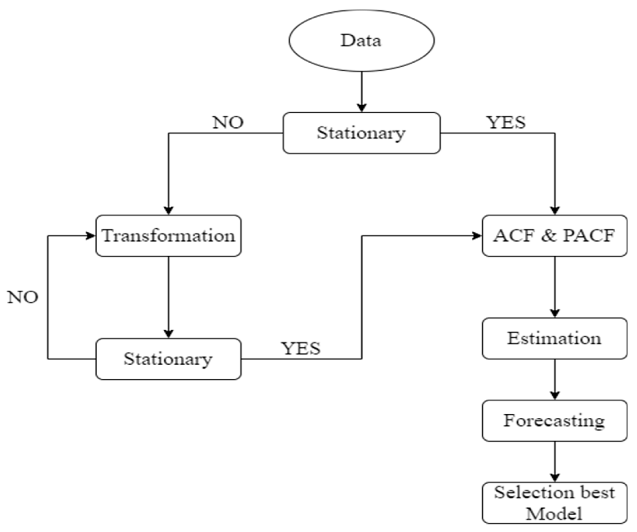
  • Stationarity test: The augmented Dickey-Fuller (ADF) test is employed to determine whether a time series is stationary or nonstationary. If the time series is nonstationary, it should be subjected to differential operation.
  • Order identification: The orders of the ARIMA model are determined by examining the autocorrelation coefficient function (ACF) and partial autocorrelation coefficient function (PACF) of the time series. Another approach Python package is the auto_arima function that conducts a systematic search across potential ARIMA hyperparameters in a stepwise manner.
  • Model fitting: The Kalman filter and the maximum likelihood function are used to estimate and fit the model's unknown parameters. Furthermore, the model is examined to see if the residual sequence contains white noise. Otherwise, the orders must be inappropriate and must be re-identified.
  • Application: The ARIMA model is utilized to forecast the SPI index, and the data is added to the training sample. Before the next forecast, the model should be updated. Figure 3 depicts the forecasting process using the best ARIMA model.

2.5. Long Short-Term Memory Neural Network

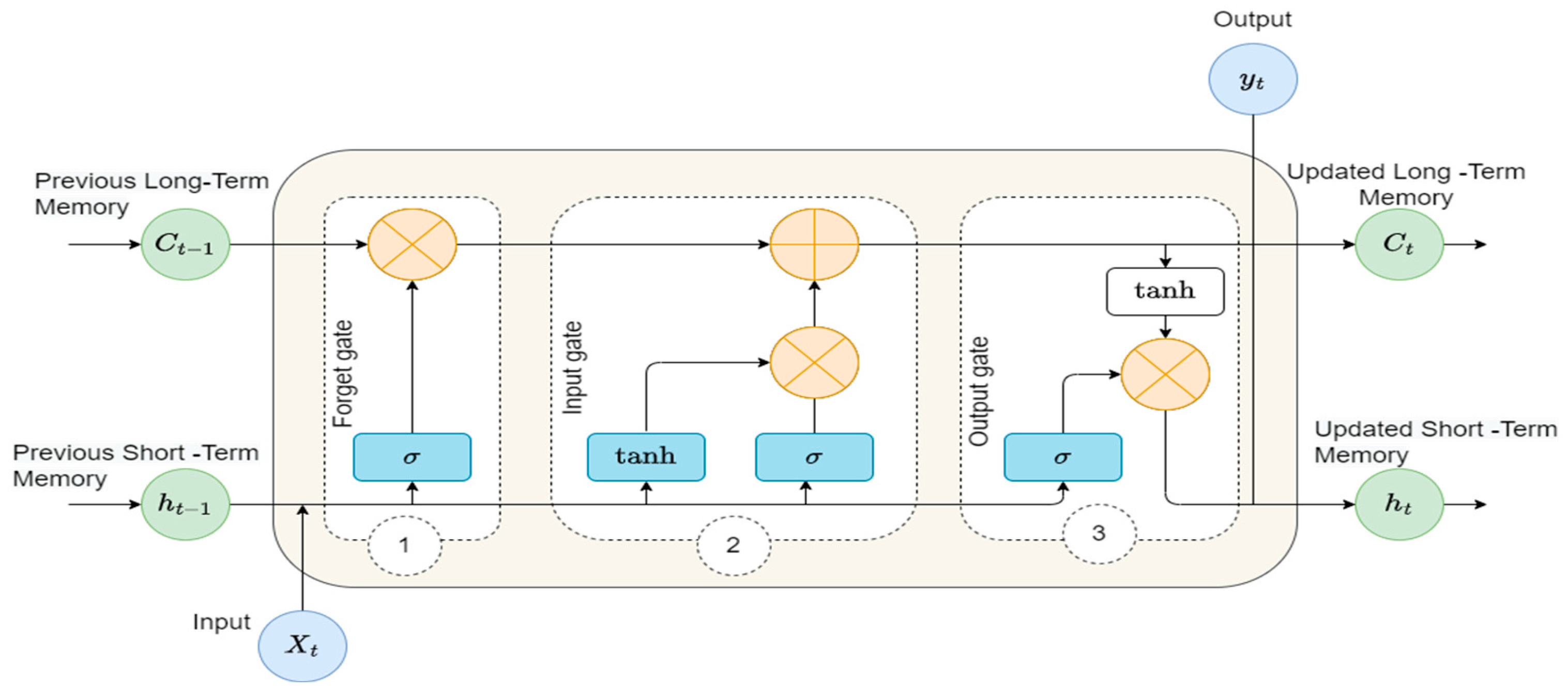
The Long Short-Term Memory (LSTM) was first proposed by Hochreiter and Schmidhuber [41] as one of the most successful recurrent neural networks (RNN) architectures. LSTM, a variant of recurrent neural networks (RNNs), incorporates a threshold mechanism consisting of an input gate, forgetting gate, and output gate. This mechanism evaluates incoming information to determine if it satisfies certain criteria, thus regulating the rate at which information is accumulated. Consequently, LSTM is capable of retaining and updating new information, effectively addressing the issue of long-term dependence. As illustrated in Figure 4, the neural unit of each LSTM is made up of the cell state, namely the long-term state c t and the short-term state h t , as well as the input gate i t , forgetting gate f t , and output gate o t .
The cell state, which can be viewed as a container for storing information, modifies and outputs the information progressively through process control of the input, forgetting, and output gates. Each cell state within a neural unit experiences the forget gate, the input gate, and the process of transferring information to the output gate. To process the current neural unit, the input gate duplicates the incoming data. The entire input consists of two components. The sigmoid activation function portion specifies which categories of input data are updated, i.e. which input data is disregarded. The hyperbolic tangent function (tanh) was utilised to produce a novel candidate value vector, which was then added to the current cell state. The mathematical procedure is defined by:
i t = σ W i   . x t . h t 1 + b i
c t = φ W c   .   x t . h t 1 + b c
The forget gate is employed to determine which information in the current state should be discarded, while the LSTM algorithm acquires the ability to instruct the network to retain information.
f t = σ W f   . x t . h t 1 + b f
The output gate is primarily responsible for controlling the output information of the present concealed state.
h t = o t φ c t
c t = i t c t + f t c t 1
o t = σ W o   . x t . h t 1 + b o
In the equation, x t represents the input, and h t signifies the network's output at time t . Meanwhile, c t represents the newly formed candidate value vectors for the tanh component at time t . The elements f t , i t , and o t pertain to the forget gate, input gates, and output gates, respectively. The matrices W f , W i , W 0 , and W c correspond to the weights associated with the forget, input, output, and memory cells. Additionally, b f , b i , b o , and b c denote the bias vectors linked to the forget, input, output, and memory cells, respectively. The function σ symbolizes the sigmoid function, while φ is indicative of the Tanh function. To acquire the optimal parameters for augmenting the performance of the LSTM model, errors and gradients are calculated using the time backpropagation technique. The backpropagation in LSTM networks entails the computation of gradients over time, the modification of network parameters, and the control of information propagation through the cell state and gates. The LSTM's ability to capture long-term dependencies in sequential data makes it highly suitable for time-series prediction.

2.6. The Development of the Hybrid CEEMDAN-ARIMA-LSTM Model

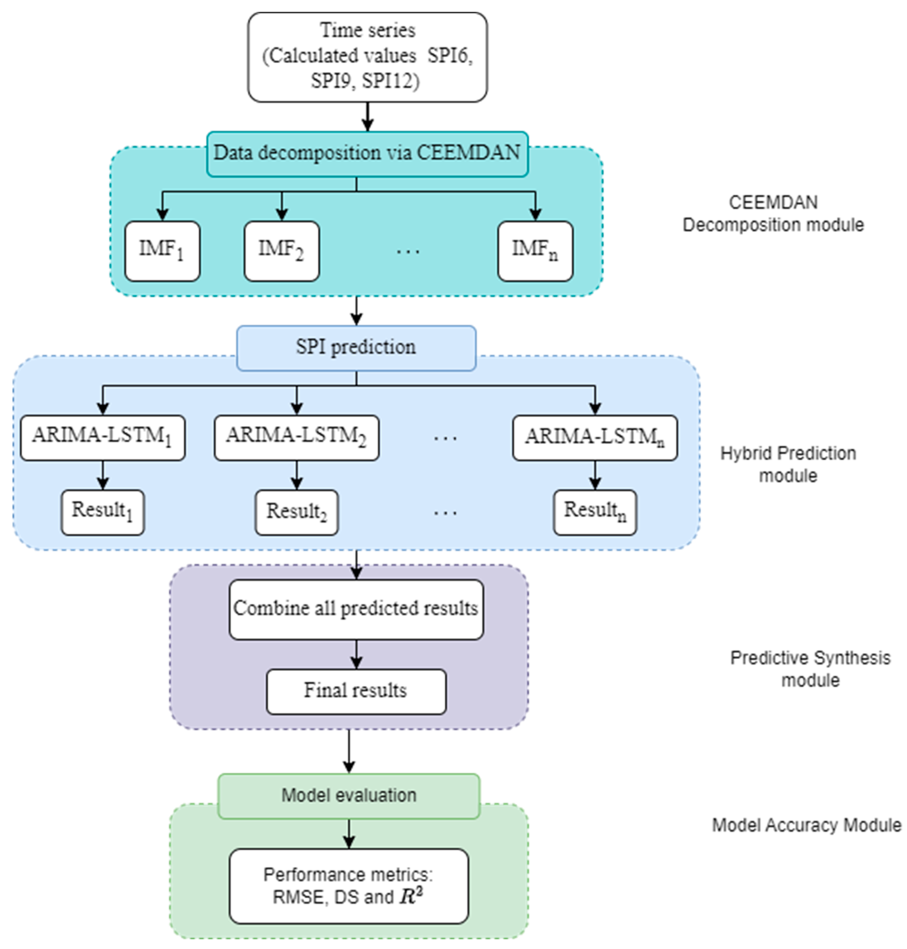
In the development of the hybrid CEEMDAN-ARIMA-LSTM model, this work utilizes the complete ensemble empirical mode decomposition with adaptive noise (CEEMDAN), autoregressive integrated moving average model (ARIMA), and long-term and short-term memory networks (LSTM). The CEEMDAN modal decomposition method is used to decompose the data at different frequencies to improve the timing characteristics reflected in the data and achieve the noise reduction effect, and the advantage of LSTM and ARIMA in time series data processing is exploited to enhance prediction accuracy. The specific procedures are listed below:
  • Decompose the original data into Intrinsic Mode Functions (IMFs) and a residual component using the CEEMDAN technique. CEEMDAN decomposes the time series into numerous oscillatory mode components with varying frequencies, capturing both high-frequency and low-frequency components, thereby making it easier for subsequent models to capture distinct patterns.
  • The ARIMA models are used to capture temporal dependencies and trends, as well as to analyse individually each of the retrieved IMFs and the residual component derived from CEEMDAN. Develop separate ARIMA models for the IMF and residual. The residual is then combined with the forecasts from the ARIMA models of each IMF to reconstruct the predicted series.
  • From the ARIMA fitted results, the calculated residuals serve as inputs of the LSTM model. Train the LSTM model using the training set to generate 1-step ahead forecasts.
  • The prediction result is derived by adding the predicted values of the high-frequency components using LSTM and the predicted value of the low-frequency components using ARIMA.
  • Repeat steps (1) to (4) for k = 2 ,   3 ,   ,   K yields the final prediction.

2.7. Model Performance Criteria

The selection of the metric to assess the performance of the suggested model is of utmost importance. The selection of metrics has a significant impact on how the performance of model algorithms is evaluated and compared. The two most frequently used performance metrics are root mean square error (RMSE) and coefficient of determination R 2 . RMSE measures the average difference between the actual and projected values, while R 2 quantifies the extent of correlation between them [42]. In addition, we utilize the concept of directional symmetry (DS) to evaluate a model's capacity to accurately predict the direction of changes in value. The metrics are mathematically defined as follows:
R M S E = 1 n i = 1 n y i y ^ i 2
R 2 = i = 1 n y ^ i y ¯ i 2 / i = 1 n y i y ¯ i 2
D S y , y ^ = 100 n 1 i = 2 n d i d i = 1 ,     i f   y i y i 1 y ^ i y ^ i 1 > 0 0 ,     o t h e r w i s e
where n is the number of data points, y i is the observed value, y ^ i is the predicted value and y ¯ i is the mean of the observation data.

3. Results and Discussion

3.1. Rainfall Data Series and Trend Analysis

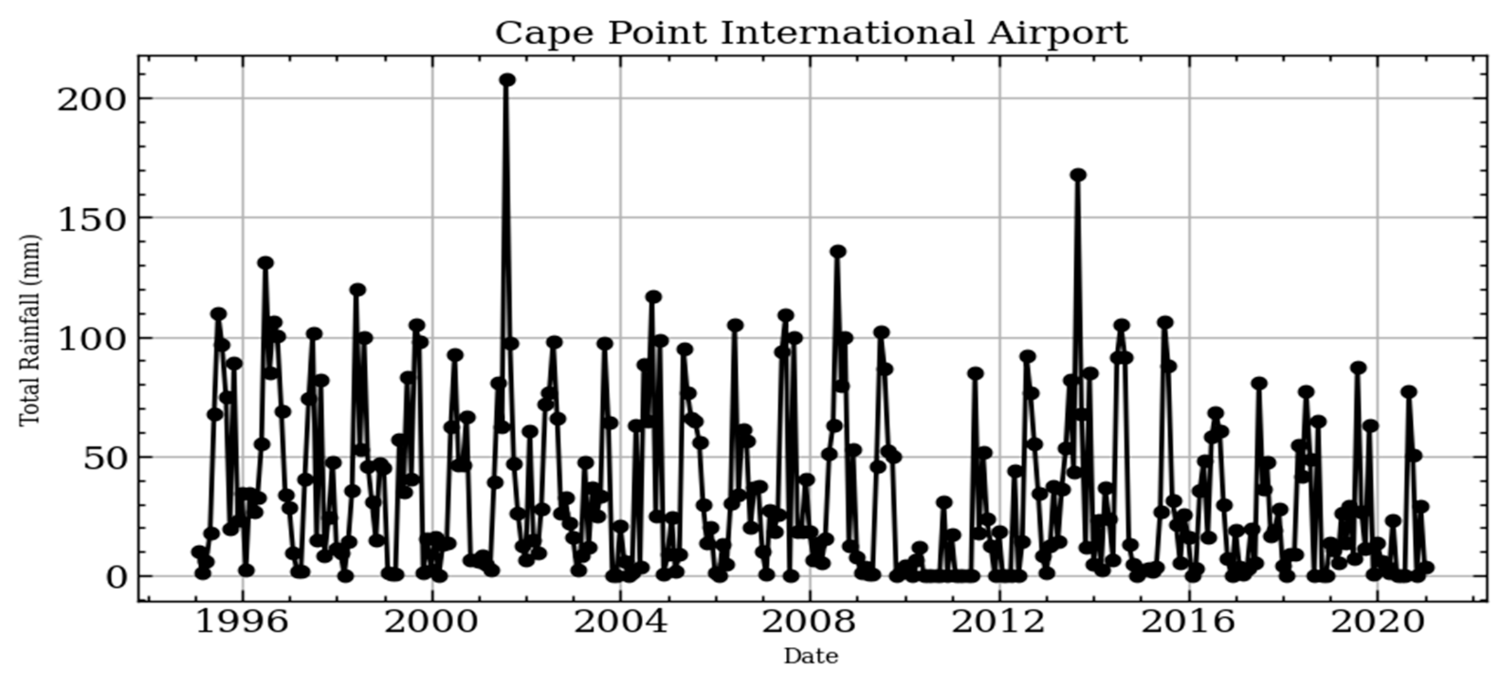
Figure 6 shows the monthly cumulative rainfall data measured at the Cape Town International Airport meteorological station in the Western Cape province of South Africa from 1995 to 2020. Typically, the monthly rainfall ranges from 0 to approximately 100 mm, with occasional instances where it exceeds 150 mm. The rainfall time series was utilised to calculate the Standardised Precipitation Index (SPI) in this research. Prior to calculating the SPI, it is crucial to evaluate the rainfall pattern across the research region. Thus, the section below will utilise innovative trend approaches to investigate rainfall trends.
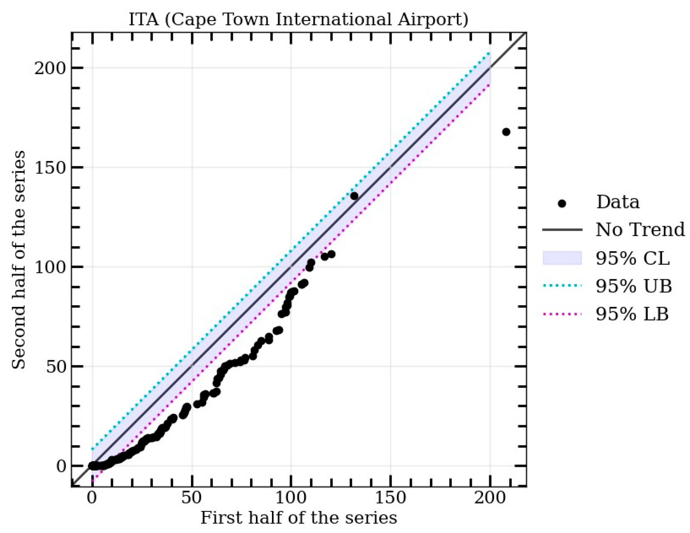
The results of the ITA analysis of monthly total rainfall for the Cape Town International Airport are presented in Figure 7 and Table 2, estimated at a 95% confidence level. The 1:1 line of the ITA, with the 95% confidence limit area shaded light blue between the 95% confidence upper limit (blue line) and the 95% confidence lower limit (purple line). According to the ITA methodology, if the slope value falls within the lower and upper limits, there is no discernible trend. In contrast, if the slope exceeds the upper limit, an increasing trend is observed, whereas a decreasing trend is indicated if the slope falls below the lower limit. The rainfall variable results in Figure 7 revealed that most of the data points were situated below the 1:1 line, indicating a significant overall decreasing trend. This finding strongly aligned with the ITA trend indicator value (-3.215) (see Table 2). Additionally, Table 2 displays a slope of -0.083, which is below the ITA 95% confidence interval. This further confirms the presence of a decreasing trend, and the significance was established at the 5% level, as the calculated p-value was lower than the alpha level (0.05). However, it should be noted that the trend seems to recover for higher rainfall values.
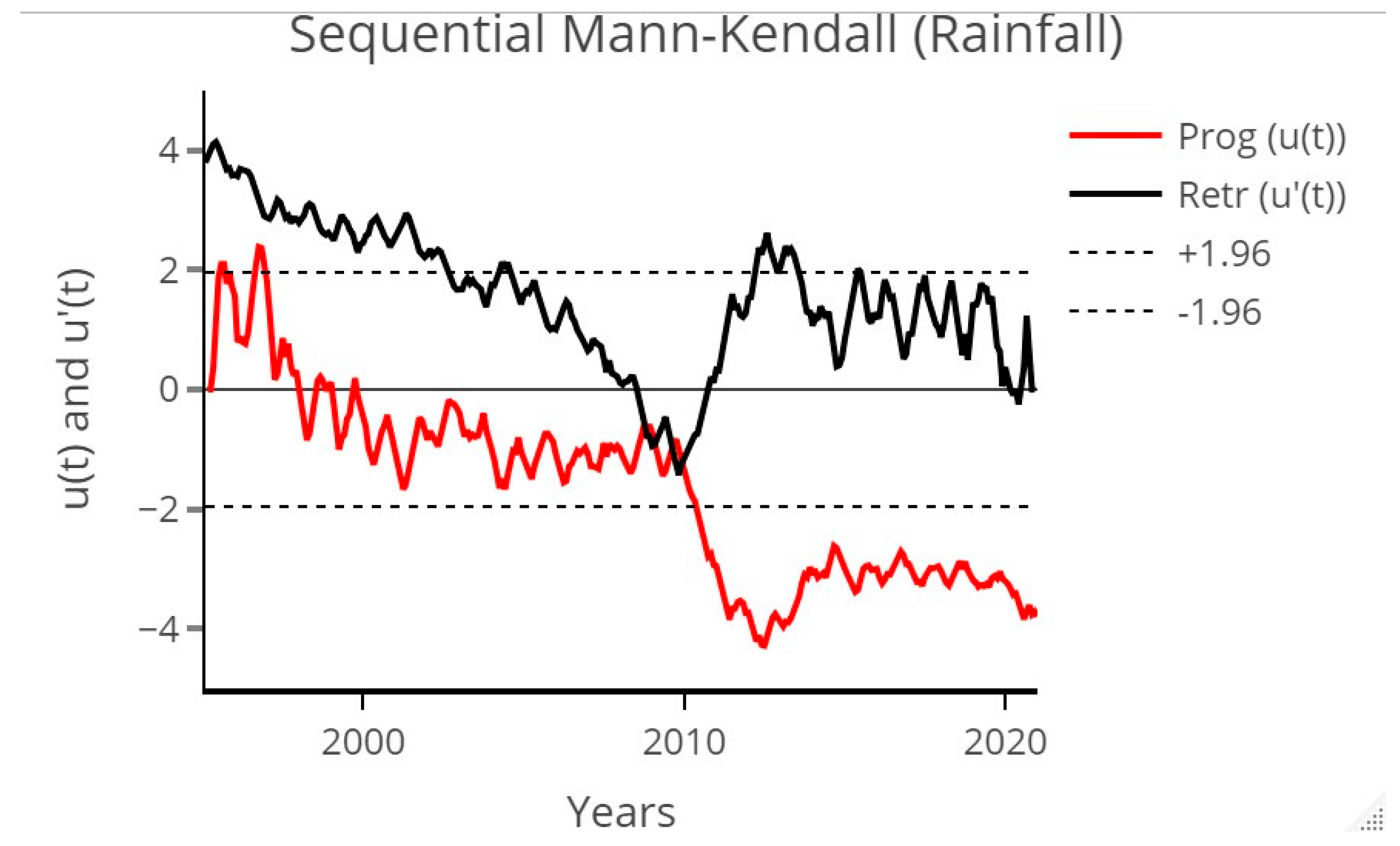
The results of the sequential Mann-Kendall (SQ-MK) test statistics for the monthly rainfall dataset of Cape Town International. In this Figure monthly values of u ( t i ) and u t i for the period from 1995 to 2020. The major trend change detection point is reported in November, where the curves of u ( t i ) and u t i   i ntersect each other. This leads to a significant downwards trend that persists from 2010 onwards. The downward trend presented by SQ-MK seems to be consistent with the ITA results presented in Figure 7 and Table 2.
The MK and MMK techniques were also applied on the total rainfall time series (see Table 3). In Table 3, the results indicate that both the MK and the MMK methods reported a significant decreasing trend with negetive Z-score values of -3.374 and -4.077, respectively, and p-values of 1.74002 × 10 04 and 4.5564 × 10 05 , respectively, which are lower than the alpha level (0.05). and in general, all these results indicate are consistent to those reported by the SQ-MK and ITA.

3.2. SPI Time Series and Forecusting Results

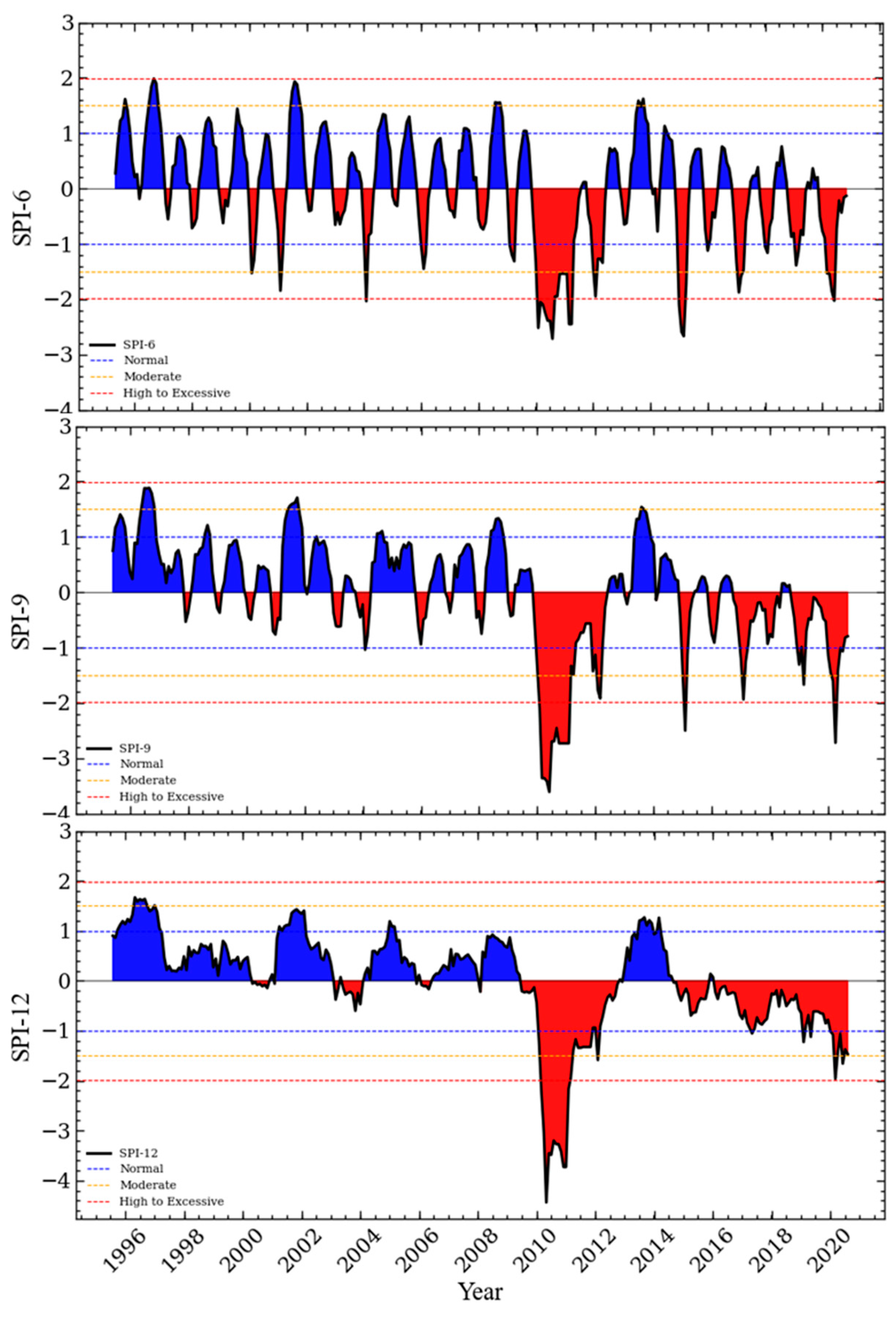
In this study, the SPI values for the 6-, 9-, and 12-month timescale were calculated using mothly total rainfall data measured at the Cape Town Internatinal Airport meteorological station in the Western Cape Region of South Africa (See Figure 6). Figure 9 illustrates the time series of SPI computed for timescales 6-months (SPI6), 9-months (SPI9), and 12-months (SPI12), respectively. In general, all SPIs (SPI6, SPI9, and SPI12) reported several episodes of moderate to high to excessive droughts in the study area. There is a broad peak of drought period that begins late 2009 and persist to 2012. SPI12 reported a persistant drought period that started in 2014, that led to day zero conditions in terms of water supply over Cape Town [43].
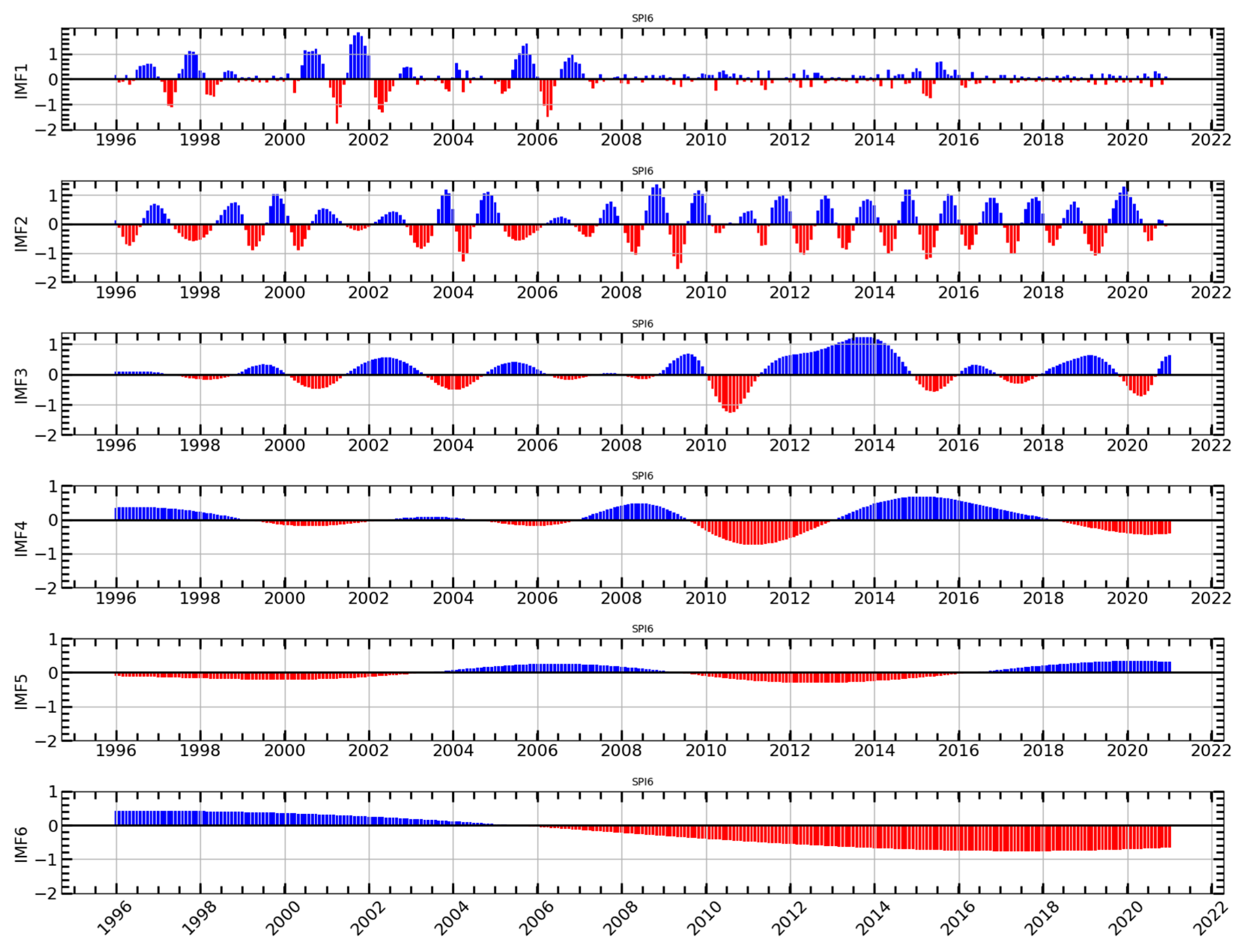
The complexity and fluctuation of the original SPI series in the model fitting and subsequent convergence of the model can be affected and thus limit the prediction accuracy. In response to the challenges, the nonlinear and nonstationary SPI series is preprocessed with the powerful method for conducting the decomposition of the series, namely CEEMDAN algorithm [44]. The decomposition of the time series is a fundamental component of the hybrid model proposed in this research for time series forecasting. As a result, CEEMDAN deconstructed the training dataset, yielding five IMF components and one trend time series. For an example of the decomposition of the time series, CEEMDAN was applied to the SPI6 time series, and the results are shown in Figure 10. While the CEEMDAN is able to present all IMFs, it is important to mention that IMF6 (which is assoiated with the Trend) seem to indicate that a downwards trend of the SPI6 time series, which could indicate that the domination of dry spells in recent over the study area.
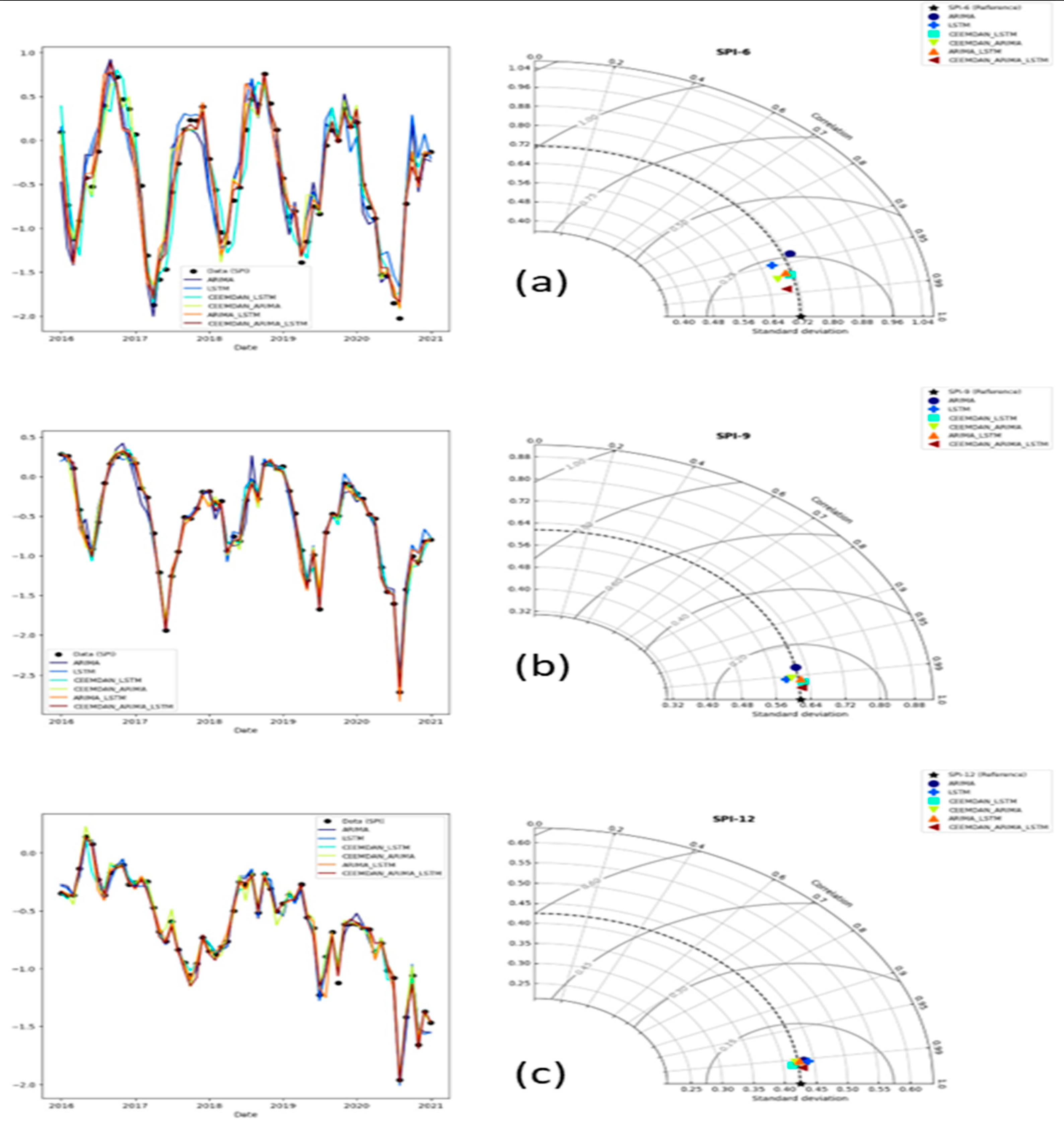
This study compared the prediction performance of models listed in Table 4 before and after time series decomposition to determine whether the effort of decomposition improves the practicality of the model's prediction performance. Figure 11 presents a comparison of the prediction results of different models, along with the original time series for SPI6, SPI9, and SPI12, as well as a Taylor diagram. Overall, all models appear to closely mimic the original SPI time series across all time scales (see Figure 11). The Taylor diagram seem to indicate an improvement in prediction accuracy after applying CEEMDAN signal decomposition method, with the CEEMDAN-ARIMA-LSTM model outperforming other models in terms of prediction accuracy across all time scales. Table 4 evaluates the comparison of prediction performance values of different models using RMSE, R 2 and DS. As the time scale increases, the RMSE values of the models decrease, while the DS values generally increase (see Table 4). This indicates that the prediction accuracy of the models gradually improves with increasing time scale, peaking at the 12-month time scale. For instance, the LSTM model implemented at SPI6 had an RMSE of 0.234 and a R 2 of 0.897, while at SPI12, it had an RMSE of 0.058 and a R 2 of 0.984. In Table 4, it can be observed that at all-time scales, the RMSE values of the CEEMDAN-ARIMA and CEEMDAN-LSTM models were lower than those of the ARIMA and LSTM models, respectively, while the R 2 values were higher than those of the single models. This indicates higher prediction accuracy of the combined model, making it more suitable for predicting multiscale SPI. At each monthly time scale, the prediction accuracy of the ARIMA-LSTM combined model was significantly higher than that of the single model, with slightly higher accuracy for SPI6, SPI9, and SPI12. For example, in SPI6, the model had an RMSE of 0.186 and a R 2 of 0.931, while in SPI9, it had an RMSE of 0.077 and a R 2 of 0.983. In SPI12, the RMSE was 0.057 and the R 2 was 0.985. It is evident that the prediction performance after the CEEMDAN decomposition is superior to that of the undecomposed models, suggesting that the SPI time series is better predicted after decomposition. Among these models, the CEEMDAN-ARIMA-LSTM model achieves the highest prediction accuracy with RMSE values ranging from 0.120 to 0.042, DS values ranging from 0.915 to 0.950, and values ranging from 0.970 to 0.995, significantly outperforming other models.

5. Conclusions

In the present study, the Mann-Kendall (MK) test and innovative trend analysis (ITA) method were utilized to analyze the trends in monthly rainfall total data at Cape Town International Airport, South Africa, for the period from 1995 to 2020. The results of the MK and MMK test indicated a significant decreasing trend in rainfall at a 95% significance level. These findings were further supported by the ITA results, with most data points falling below the 1:1 line, indicating a downward trend. Both the SQ-MK and ITA methods indicates a significant downwards trend of rainfall in the study area for most of the years. The recovery of the downwards trend seems to be observed during the period after the 2014-2016 strong El Niño years. Moreover, this study used rainfall data to compute the SPI and used this data train and forecast the SPI data at multiscale using ARIMA and LSTM. To achieve accurate SPI forecasts, the CEEMDAN signal processing algorithm was integrated with the ARIMA, LSTM, and ARIMA-LSTM hybrid model. A comprehensive comparative analysis of the prediction outcomes was conducted (see Figure 11 and Table 4). The results revealed that all models produced good performance in predicting SPI in all timescales. Performance steadily increased as the timescale increased presumably because of lower noise levels for higher SPI time scales. Throughout multiple timescales, the CEEMDAN combine hybrid model consistently outperformed the individual models. Specifically, for SPI12, the hybrid model exhibited RMSE values exceeding 0.97, highlighting CEEMDAN's ability to handle non-stationary and non-linear data characteristics, thereby improving predictability. Additionally, as depicted in Figure 11, the drought index predictions derived from the hybrid CEEMDAN-ARIMA-LSTM model are reported to have a superior prediction accuracy compared to other models across all timescales. It is evident that the combination of CEEMDAN with ARIMA, LSTM, and ARIMA-LSTM has the potential to significantly enhance the accuracy of meteorological drought forecasting.
The findings presented in this study seem to indicate that potential of hybrid models in predicting climate change patterns, which could be key for early warning systems. This could be useful for planning and policy decisions related to agricultural production and tourism management. Furthermore, analyzing climate parameters can help predict climate changes, especially drought and abnormal wet spells. And future investigations should explore the predictability of the standardized precipitation evapotranspiration index (SPEI) to assess the applicability of the combined model.

Author Contributions

For research articles with several authors, a short paragraph specifying their individual contributions must be provided. The following statements should be used “Conceptualization, S.S. and M.N.; methodology, S.S. and M.N.; software, S.F.; validation, M.N., S.R. and S.M.; formal analysis, S.F.; writing—original draft preparation, S.S.; writing—review and editing, M.N; S.R.; S.M and S.F.; supervision, M.N; S.R. and S.M. All authors have read and agreed to the published version of the manuscript.

Funding

This research received no external funding.

Data Availability Statement

Not applicable

Acknowledgments

In this section, you can acknowledge any support given which is not covered by the author contribution or funding sections. This may include administrative and technical support, or donations in kind (e.g., materials used for experiments).

Conflicts of Interest

The authors declare no conflict of interest.

References

  1. Fang, Ouya, Qi-Bin Zhang, Yann Vitasse, Roman Zweifel, and Paolo Cherubini. "The frequency and severity of past droughts shape the drought sensitivity of juniper trees on the Tibetan plateau." Forest Ecology and Management 486 (2021): 118968. [CrossRef]
  2. Murgatroyd, Anna, Helen Gavin, Olivia Becher, Gemma Coxon, Doug Hunt, Emily Fallon, Jonny Wilson, Gokhan Cuceloglu, and Jim W. Hall. "Strategic analysis of the drought resilience of water supply systems." Philosophical Transactions of the Royal Society A 380, no. 2238 (2022): 20210292.
  3. Garrick, Dustin, Lucia De Stefano, Winston Yu, Isabel Jorgensen, Erin O’Donnell, Laura Turley, Ismael Aguilar-Barajas et al. "Rural water for thirsty cities: A systematic review of water reallocation from rural to urban regions." Environmental Research Letters 14, no. 4 (2019): 043003.
  4. Vorosmarty, Charles J., Pamela Green, Joseph Salisbury, and Richard B. Lammers. "Global water resources: vulnerability from climate change and population growth." science 289, no. 5477 (2000): 284-288.
  5. Hall, Jim W., David Grey, Dustin Garrick, Fai Fung, Casey Brown, Simon J. Dadson, and Claudia W. Sadoff. "Coping with the curse of freshwater variability." Science 346, no. 6208 (2014): 429-430.
  6. Murgatroyd, A., and J. W. Hall. "Regulation of freshwater use to restore ecosystems resilience." Climate Risk Management 32 (2021): 100303.
  7. Jin, Li, Paul G. Whitehead, Gianbattista Bussi, Feyera Hirpa, Meron Teferi Taye, Yosef Abebe, and Katrina Charles. "Natural and anthropogenic sources of salinity in the Awash River and Lake Beseka (Ethiopia): modelling impacts of climate change and lake-river interactions." Journal of Hydrology: Regional Studies 36 (2021): 100865. [CrossRef]
  8. Hall, Jim W., Edoardo Borgomeo, Alexa Bruce, Manuela Di Mauro, and Mohammad Mortazavi-Naeini. "Resilience of water resource systems: lessons from England." Water Security 8 (2019): 100052.
  9. Khan, Md Munir Hayet, Nur Shazwani Muhammad, and Ahmed El-Shafie. "Wavelet based hybrid ANN-ARIMA models for meteorological drought forecasting." Journal of Hydrology 590 (2020): 125380.
  10. Han, Ping, Pengxin Wang, Miao Tian, Shuyu Zhang, Junming Liu, and Dehai Zhu. "Application of the ARIMA models in drought forecasting using the standardized precipitation index." In Computer and Computing Technologies in Agriculture VI: 6th IFIP WG 5.14 International Conference, CCTA 2012, Zhangjiajie, China, October 19-21, 2012, Revised Selected Papers, Part I 6, pp. 352-358. Springer Berlin Heidelberg, 2013.
  11. Ding, Yan, Guoqiang Yu, Ran Tian, and Yizhong Sun. "Application of a hybrid CEEMD-LSTM model based on the standardized precipitation index for Drought forecasting: the case of the Xinjiang Uygur Autonomous Region, China." Atmosphere 13, no. 9 (2022): 1504.
  12. Liu, Ming-De, Lin Ding, and Yu-Long Bai. "Application of hybrid model based on empirical mode decomposition, novel recurrent neural networks and the ARIMA to wind speed prediction." Energy Conversion and Management 233 (2021): 113917.
  13. Poornima, S., and M. Pushpalatha. "Drought prediction based on SPI and SPEI with varying timescales using LSTM recurrent neural network." Soft Computing 23 (2019): 8399-8412.
  14. Dikshit, Abhirup, Biswajeet Pradhan, and Abdullah M. Alamri. "Long lead time drought forecasting using lagged climate variables and a stacked long short-term memory model." Science of The Total Environment 755 (2021): 142638.
  15. Balti, Hanen, Ali Ben Abbes, Nedra Mellouli, Yanfang Sang, Imed Riadh Farah, Myriam Lamolle, and Yanxin Zhu. "Big data based architecture for drought forecasting using LSTM, ARIMA, and Prophet: Case study of the Jiangsu Province, China." In 2021 International Congress of Advanced Technology and Engineering (ICOTEN), pp. 1-8. IEEE, 2021.
  16. Wang, Zhi-Yu, Jun Qiu, and Fang-Fang Li. "Hybrid models combining EMD/EEMD and ARIMA for Long-term streamflow forecasting." Water 10, no. 7 (2018): 853.
  17. Mathivha, Fhumulani, Caston Sigauke, Hector Chikoore, and John Odiyo. "Short-term and medium-term drought forecasting using generalized additive models." Sustainability 12, no. 10 (2020): 4006. [CrossRef]
  18. Guoyang, Zhao, Tu Xinjun, Wang Tian, X. I. E. Yuting, and M. O. Xiaomei. "Drought Prediction Based on Artificial Neural Network and Support Vector Machine." Pearl River 42, no. 4 (2021): 1.
  19. Wu, Guodong, Jun Zhang, and Heru Xue. "Long-Term Prediction of Hydrometeorological Time Series Using a PSO-Based Combined Model Composed of EEMD and LSTM." Sustainability 15, no. 17 (2023): 13209.
  20. Xu, Dehe, Yan Ding, Hui Liu, Qi Zhang, and De Zhang. "Applicability of a CEEMD–ARIMA Combined Model for Drought Forecasting: A Case Study in the Ningxia Hui Autonomous Region." Atmosphere 13, no. 7 (2022): 1109.
  21. Mann, H. B. (1945). Nonparametric tests against trend. Econometrica: Journal of the econometric society, 245-259.
  22. Kendall, M.G. Rank Correlation Methods; Griffin: London, UK, 1975.
  23. Seenu, PZ, & Jayakumar KV. (2021). Comparative study of innovative trend analysis technique with Mann-Kendall tests for extreme rainfall. Arabian Journal of Geosciences, 14, 1-15.
  24. Körük, A. E., Kankal, M., Yıldız, M. B., Akçay, F., Şan, M., & Nacar, S. (2023). Trend analysis of precipitation using innovative approaches in northwestern Turkey. Physics and Chemistry of the Earth, Parts A/B/C, 131, 103416.
  25. Mbatha, N., & Xulu, S. (2018). Time series analysis of MODIS-Derived NDVI for the Hluhluwe-Imfolozi Park, South Africa: Impact of recent intense drought. Climate, 6(4), 95.
  26. Onoz, B., & Bayazit, M. (2003). The power of statistical tests for trend detection. Turkish journal of engineering and environmental sciences, 27(4), 247-251.
  27. Othman, M. A., Zakaria, N. A., Ghani, A. A., Chang, C. K., & Chan, N. W. (2016). Analysis of trends of extreme rainfall events using Mann Kendall test: a case study in Pahang and Kelantan river basins. Jurnal Teknologi, 78(9-4).
  28. Hamed, K. H., & Rao, A. R. (1998). A modified Mann-Kendall trend test for autocorrelated data. Journal of hydrology, 204(1-4), 182-196.
  29. Kumar, S., Machiwal, D., & Dayal, D. (2017). Spatial modelling of rainfall trends using satellite datasets and geographic information system. Hydrological Sciences Journal, 62(10), 1636-1653.
  30. Singh, R. N., Sah, S., Das, B., Potekar, S., Chaudhary, A., & Pathak, H. (2021). Innovative trend analysis of spatio-temporal variations of rainfall in India during 1901–2019. Theoretical and Applied Climatology, 145(1), 821-838.
  31. Sneyers, R. (1991) On the Statistical Analysis of Series of Observations; Technical Note No. 143, WMO No. 415; World Meteorological Organization: Geneva, Switzerland, p. 192.
  32. Bisai, D., Chatterjee, S., & Khan, A. (2014). Detection of recognizing events in lower atmospheric temperature time series (1941-2010) of Midnapore Weather Observatory, West Bengal, India. J Environ Earth Sci, 4(3), 61-66.
  33. Şen, Z. (2012). Innovative trend analysis methodology. Journal of Hydrologic Engineering, 17(9), 1042-1046.
  34. McKee, Thomas B., Nolan J. Doesken, and John Kleist. "The relationship of drought frequency and duration to time scales." In Proceedings of the 8th Conference on Applied Climatology, vol. 17, no. 22, pp. 179-183. 1993.
  35. Belayneh, A., and J. Adamowski. "Standard precipitation index drought forecasting using neural networks, wavelet neural networks, and support vector regression." Applied computational intelligence and soft computing 2012 (2012): 6-6.
  36. Elbeltagi, Ahmed, Chaitanya B. Pande, Manish Kumar, Abebe Debele Tolche, Sudhir Kumar Singh, Akshay Kumar, and Dinesh Kumar Vishwakarma. "Prediction of meteorological drought and standardized precipitation index based on the random forest (RF), random tree (RT), and Gaussian process regression (GPR) models." Environmental Science and Pollution Research 30, no. 15 (2023): 43183-43202. [CrossRef]
  37. Lloyd-Hughes, Benjamin, and Mark A. Saunders. "A drought climatology for Europe." International Journal of climatology: a journal of the royal meteorological society 22, no. 13 (2002): 1571-1592.
  38. Torres, María E., Marcelo A. Colominas, Gaston Schlotthauer, and Patrick Flandrin. "A complete ensemble empirical mode decomposition with adaptive noise." In 2011 IEEE international conference on acoustics, speech and signal processing (ICASSP), pp. 4144-4147. IEEE, 2011.
  39. Box, George EP, Gwilym M. Jenkins, and WISCONSIN UNIV MADISON DEPT OF STATISTICS. "Time Series Analysis Forecasting and Control." (1970).
  40. Sharma, Rishi Raj, Mohit Kumar, Shishir Maheshwari, and Kamla Prasan Ray. "EVDHM-ARIMA-based time series forecasting model and its application for COVID-19 cases." IEEE Transactions on Instrumentation and Measurement 70 (2020): 1-10.
  41. Hochreiter, Sepp, and Jürgen Schmidhuber. "Long short-term memory." Neural computation 9, no. 8 (1997): 1735-1780.
  42. Alexander, David LJ, Alexander Tropsha, and David A. Winkler. "Beware of R 2: simple, unambiguous assessment of the prediction accuracy of QSAR and QSPR models." Journal of chemical information and modeling 55, no. 7 (2015): 1316-1322. [CrossRef]
  43. Calverley, C. M., & Walther, S. C. (2022). Drought, water management, and social equity: Analyzing Cape Town, South Africa's water crisis. Frontiers in Water, 4, 910149.
  44. Sun, Y., & Liu, J. (2022). Aqi prediction based on ceemdan-arma-lstm. Sustainability, 14(19), 12182.
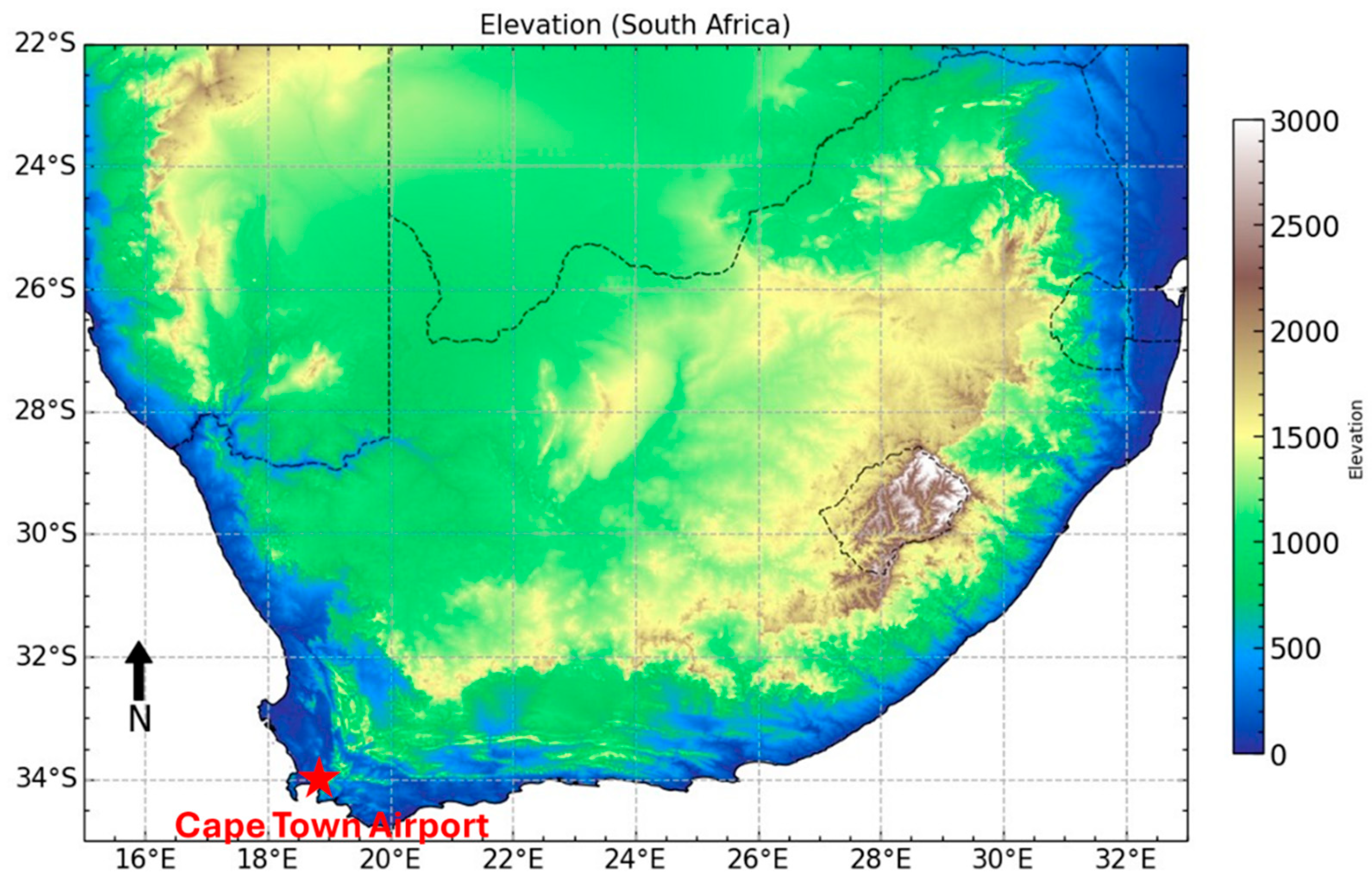
Figure 1. The study area map. Cape Town International Airport is indicated by a red star.
Preprints 112904 g001
Figure 3. The model selection process by forecasting.
Preprints 112904 g003
Figure 4. The LSTM architecture.
Preprints 112904 g004
Figure 5. Schematic structure of the developed hybrid CEEMDAN-ARIMA-LSTM model.
Preprints 112904 g005
Figure 6. Time series of the monthly rainfall.
Preprints 112904 g006
Figure 7. Innovative trend analysis of monthly total rainfall data measured over Cape Town International Airport meteorological station, South Africa.
Preprints 112904 g007
Figure 8. Sequential values of the statistics u(t) (red line) and u’(t) (black line) from the Mann-Kendall test for monthly rainfall.
Preprints 112904 g008
Figure 9. Observed SPI values at the 6-, 9-, and 12-month timescales.
Preprints 112904 g009
Figure 10. The CEEMDAN decomposition results of SPI6 sequence.
Preprints 112904 g010
Figure 11. The time series of observations and forecasts for the SPI prediction (Left) and their Taylor diagram plots at different time scales (Right) (a) SPI-6, (b) SPI-9, and (c) SPI-12.
Preprints 112904 g011
Table 1. Climate classification based on Standardized Precipitation Index (SPI) values.
SPI Value Class Probability (%)
SPI ≥ 2.00 Extremely wet 2.3
1.5 ≤ SPI < 2.00 Severely wet 4.4
SPI < 1.50 Moderately wet 9.2
SPI < 1.00 Mildly wet 34.1
−1.00 ≤ SPI < 0.00 Mild drought 34.1
−1.50 ≤ SPI < −1.00 Moderate drought 9.2
−2.00 ≤ SPI < −1.50 Severe drought 4.4
SPI < −2.00 Extreme drought 2.3
Table 2. Trend results in rain values by ITA.
ITA Variables Values
Trend slope -0.083083
Trend indicator -3.214672
Correlation 0.985378
Slope standard deviation 0.002202
Confidence Limit ( ± ) 0.003415
Table 3. MK and MMK Statistics for Rainfall of Cape Town International Airport.
Variables Mann-Kendall Modified Mann-Kendall
slope 0.04810127 0.04810127
S 6909.0 6909.0
Var(s) 3386141.0 2870533.483
τ 0.142407 0.142407
z-value 3.7540 5 * 4.07728 5 *
p-value 1.74002 × 10 04 * 4.5564 × 10 05 *
Decision (Trend) Decreasing Decreasing
* Significant at 5% level of significance.
Table 4. Comparison of the observed and predicted values of the models using statistical criteria.
Model SPI-6 SPI-9 SPI-12
RMSE R 2 DS RMSE R 2 DS RMSE R 2 DS
ARIMA 0.262 0.872 0.867 0.118 0.964 0.850 0.059 0.981 0.867
LSTM 0.234 0.897 0.883 0.081 0.984 0.883 0.058 0.984 0.883
ARIMA-LSTM 0.186 0.931 0.883 0.077 0.983 0.867 0.057 0.985 0.900
CEEMDAN-ARIMA 0.169 0.945 0.850 0.083 0.983 0.833 0.054 0.984 0.933
CEEMDAN- LSTM 0.178 0.938 0.800 0.066 0.987 0.917 0.047 0.989 0.950
CEEMDAN-ARIMA-LSTM 0.121 0.972 0.950 0.044 0.991 0.917 0.042 0.995 0.950
Disclaimer/Publisher’s Note: The statements, opinions and data contained in all publications are solely those of the individual author(s) and contributor(s) and not of MDPI and/or the editor(s). MDPI and/or the editor(s) disclaim responsibility for any injury to people or property resulting from any ideas, methods, instructions or products referred to in the content.
Copyright: This open access article is published under a Creative Commons CC BY 4.0 license, which permit the free download, distribution, and reuse, provided that the author and preprint are cited in any reuse.
Prerpints.org logo

Preprints.org is a free preprint server supported by MDPI in Basel, Switzerland.

Subscribe

© 2024 MDPI (Basel, Switzerland) unless otherwise stated