1. Introduction
The most convincing and authentic law of energy goes to state that “Energy can neither be created nor destroyed" [
1]. The only human venture in the energy cycle is limited to converting it into one form to another for specific utility. In this venture, since the beginning of the industrial period, fossil fuels have been used and converted into different forms, including, electrical energy, steam, and locomotion. It is expected that these sources of energy will eventually run out. Renewable energy sources, primarily solar radiation, have recently emerged as the energy source of most hope. Household users, organizations, and industries alike are investing in solar energy infrastructure [
2,
3]. It is an interesting area of research to collect data regarding solar energy and analyze it to find insights into it. The Open Data project of Saudi Arabia collects one such data and is available for public consumption. In this paper, this data is targeted for analysis. The main objective is to study the impact of meteorological variables on solar power generation and develop a predictive model for Global Horizontal Irradiance (GHI). It is assumed that the accuracy of solar energy forecasts and energy management techniques can be improved by comprehending the impact of various meteorological elements.
Air temperature, wind speed, relative humidity, and barometric pressure are examples of meteorological variables that are important in determining how much solar radiation reaches the Earth’s surface. These elements can affect how well solar panels work, for example, temperature and humidity have an impact on photovoltaic cell efficiency [
4]. In this research, the effect of these variables on GHI is quantified through an analysis of Saudi Arabia’s Open Data project, which will allow for more precise projections of solar power generation.
The paper explores machine learning algorithms for predictive modeling. This involves using statistical and supervised machine learning techniques specifically the random forest regressor with the XGBoost algorithm [
5] to forecast solar radiation levels based on historical meteorological data. The Random Forest Regressor is chosen for its ability to handle complex interactions between variables and its robustness against over fitting. By training this model on the provided datasets. The research aims to observe the accuracy in predicting GHI and compute coefficients of meteorological variables. This is expected to facilitate better planning, installation, data collection, and management of solar energy resources. This research not only highlights the potential of renewable energy but also underscores the importance of data-driven approaches in addressing the challenges of energy sustainability.
The paper is organized as follows:
Section 2, collects the background research work in this field and organizes it under literature review.
Section 3 discusses the data schema, methodology and early visualizations of the data to get initial insights into the data.
Section 4 addresses the model construction. It discusses the random forest algorithm and how it is mapped to the current data set to create trees and the random forest.
Section 5 introduces the analytic dashboard and its instance.
Section 6 is about results and discussion on them. This section discusses, correlation analysis, meteorological analysis and predictive analysis. The section 6 also presents GHI estimation using meteorologic model coefficients.Inferences based on the confusion matrix are drawn in this section. The last section is about conclusion and future work. It is presented in
section 7.
2. Literature Review
Several studies have investigated the relationship between meteorological variables and solar power generation [
6,
7]. Factors such as temperature, wind speed, humidity, and atmospheric pressure significantly affect solar radiation and, consequently, the efficiency of solar panels[
8] [
9]. Machine learning techniques, including Random Forests, Support Vector Machines, and Neural Networks, have been widely used to model and predict solar energy output[
10,
11,
12]. A review of the relevant literature, in the context of this paper, is provided in this section.
A comprehensive report on global renewable energy problems, opportunities, and trends is presented in these two reports [
2,
3]. The report [
2] emphasizes the increasing investment in renewable energy infrastructure. [
3] Provides analysis and forecasts for renewable energy deployment from 2020 to 2025. It discusses the role of policy frameworks and market dynamics in accelerating renewable energy adoption. The report highlights the need for continued investment and innovation to meet global climate goals.
In [
4] a novel model called the SUNY model is proposed. It is a valuable tool for estimating solar irradiance. It combines satellite-based models with ground-based measurements. The paper argues that this combined method can enhance the accuracy of solar resource assessments. The study emphasizes the importance of ongoing validation and refinement of satellite models to serve the energy sector in a better way. The accuracy assessment and claim in this paper are trivialized by the fact that it uses only statistical measures and misses out on the insights from machine learning algorithms
[
5] is a seminal source on the random forest algorithm. This paper has had a profound impact on the field of machine learning, establishing Random Forest as a standard method in Predictive Modeling.
The impact of meteorological variables on solar energy is studied in [
8] and [
9]. Article [
8] examines past and present developments in solar irradiance and PV power forecasting, emphasizing the advancement of methods and the significance of precise meteorological data. It makes use of text mining to pinpoint important advancements and difficulties, such as the requirement for real-time forecasting and data quality.
The paper [
9] provides a comprehensive overview of micro-meteorology, which involves the study of atmospheric phenomena on a small scale, particularly within the lower atmosphere close to the Earth’s surface.It presents case studies on the role and impact of micro-meteorological data in the new power systems, emphasizing its growing importance in energy management and optimization.It highlights how micro-meteorological data, such as temperature, wind speed, and solar irradiance at a granular level, are crucial for accurately forecasting renewable energy outputs, managing grid stability, and optimizing power system operations.The paper addresses the importance of technology integration of weather data with IoT and AI.
Articles [
10,
11,
12] address the application of random forest algorithms for predictive analytics. The work in [
10] applies Random Forest Algorithm (RFA) to imbalanced datasets. The authors propose modifications to the standard RFA to better manage class imbalance, including techniques like balanced bootstrapping and cost-sensitive learning. They demonstrate that their method improves performance on imbalanced datasets compared to traditional methods. In [
11] split points and feature selections are completely randomized unlike in the traditional algorithm [
5]. The authors [
11] call it an “Extremely Random Forest Algorithm (ERFA). It is demonstrated that extreme randomization contributes to the computational efficiency, accuracy, and robustness of the algorithm. In [
12], RFA is applied in institutional research, forecasting learning outcomes, student performance, etc. It is concluded that the RFA outperforms traditional regression models in terms of handling non-linearity, and complexity of relationships.
The book [
13] is a comprehensive source for understanding data. It provides a nuanced discussion of open data, big data, and data infrastructures. It discusses the role of them in reshaping various domains including research. It addresses the ethical, social, and technical challenges that this data poses. In [
14] the authors examine the effects of data quality, system quality, and service quality of open government data (OGD) on citizens’ trust. The paper claims to have conducted a quantitative study based on a comprehensive questionnaire distributed among 200 citizens from 27 nationalities. The paper suggests the authorities of OGD be more adept concerning OGD in creating trust. [
15] presents OpenSolar, a platform intended to improve the open use of solar datasets. OpenSolar facilitates improved research, innovation, and cooperation by offering a central platform for a variety of solar statistics. The study emphasizes the necessity of ongoing initiatives to support data openness and accessibility in the solar energy industry while highlighting the opportunities and difficulties in accomplishing this goal.
In [
16] a hybrid AI model that combines Long Short Term Memory (LSTM) and Gated Recurrent Units (GRU) is proposed. The objective focus is to forecast short term solar energy with high accuracy, and reliability. The authors compare both LSTM and GRU and report on the hybrid LSTM-GRU model. It is claimed that the proposed model outperforms the traditional solar energy forecasting models. The hybrid model captures complex temporal patterns and dependencies in solar energy.
In [
17] Support Vector Machine (SVM) is applied for solar energy forecasting.The combination of advanced machine learning techniques and big data analytics is explored in this work. The findings suggest that SVM, supported by big data analytics, can significantly enhance forecasting capabilities. The authors compare the forecasting ability of SVM with other machine learning algorithms and claim SVM’s superiority. The big data approach makes the proposed architecture scalable and robust. The authors highlight the importance of their work in solar energy technology and grid management.
In[
18] A two-step approach is proposed that combines both weather records and weather forecast data to predict generated solar power. The authors claim that this philosophy of combining data sources improves model performance. The claimed
value is 70.5%
[
19,
20], and [
21] are the three resources for programming and implementation. The book [
19], provides all Python programming and skill-related information that is required for coding. [
20] is a seminal paper that introduces the specialized world of machine learning to non-specialists through its libraries, APIs, and documentation. The tutorial in [
21] provides useful information about how to incorporate Python scripts into Power BI.
The review suggests that, there is a plethora of literature and resources to conduct such research, but the application case study is unique, and specific observations are required to be produced. The work presented in this paper becomes relevant and distinct of its kind for this reason.
3. The Data & the Analytic Plan
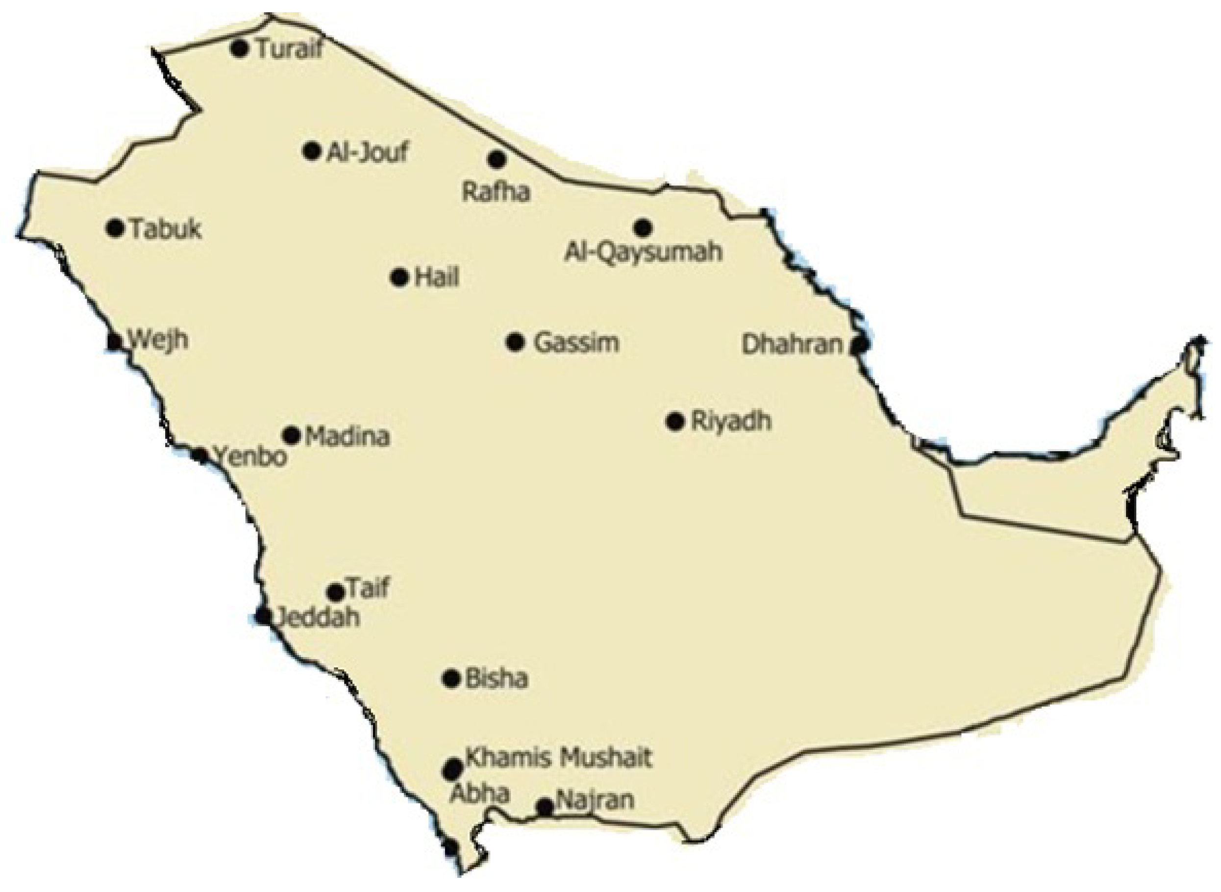
The dataset used in this study comprises meteorological data from various sites in Saudi Arabia. The following map in
Figure 1 shows the data collection centers.
The northern region is more arid than the southern region. The western region has boundaries with the Red Sea. The eastern side has the Arabian Sea near Dammam. Universities and research centers located in these geographical areas collect solar energy data in a consistent format as per a fixed schema. The government, as per its Open data policy releases this data on its
website. In this research data from all such centers is cleaned and combined to subject it for data analysis.
3.1. About the Data
The data includes parameters such as air temperature, wind speed, wind direction, relative humidity, barometric pressure, Direct Normal Irradiance (DNI), Diffuse Horizontal Irradiance (DHI), and Global Horizontal Irradiance (GHI). The dataset schema is as follows:
Table 1.
Data Schema:Attributes of the data.
Table 1.
Data Schema:Attributes of the data.
| S No |
Column Attribute |
Data Type |
| 1 |
Site: Location identifier |
Categorical |
| 2 |
Latitude: Geographical latitude of the site |
Numeric |
| 3 |
Longitude: Geographical longitude of the site |
Numeric |
| 4 |
Date: Timestamp of the recorded data |
Numeric |
| 5 |
Air Temperature (C): Ambient temperature in degrees Celsius |
Numeric |
| 6 |
Wind Direction at 3m (°N): Wind direction at 3 meters height in degrees North |
Numeric |
| 7 |
Wind Speed at 3m (m/s): Wind speed at 3 meters height in meters per second |
Numeric |
| 8 |
Relative Humidity (%): Relative humidity percentage |
Numeric |
| 9 |
Barometric Pressure (mB): Atmospheric pressure in millibars |
Numeric |
| 10 |
DHI (Wh/m²): Diffuse Horizontal Irradiance in watt-hours per square meter |
Numeric |
| 11 |
DNI (Wh/m²): Direct Normal Irradiance in watt-hours per square meter |
Numeric |
| 12 |
GHI (Wh/m²): Global Horizontal Irradiance in watt-hours per square meter |
Numeric |
Given the data and its schema, the following visualizations and analytical insights are planned. Time Series Plots, Correlation heat maps, Box Plots, Bar charts, Line plots, predictive models, Classification, regression analysis, clustering, anomaly detection, optimization, and impact analysis.
3.2. The methodology
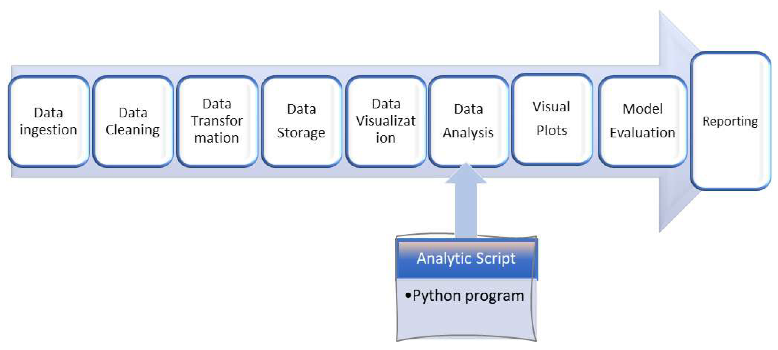
Data ingestion is the collection and importation of data from the Open Data URL. There are multiple data sets each one for a specific geographic location and the collection center. These data sets have the same schema. The schema details are discussed in section 2 above. Each of these files is extracted into one folder/directory. This completes data ingestion. A web scraper with the given URL extracts all the open data files and dumps them into one directory.
Figure 2.
Data Analytic Pipeline:The methodology
Figure 2.
Data Analytic Pipeline:The methodology
Data cleaning involves the following targeted tasks:
Removing the top 10 lines of each file
Then promoting the first line as column header
Reading the first file and appending all other files to it to form one Combined single CSV file.
Removing duplicates from this combined file
Date formatting from “d/m/Y H:M:S” to “d-m-Y” form.
Missing value substitution by the strategy of the mean of the column.
A data preprocessing script automatically performs these tasks. Finally, manual inspection is carried out to ensure the data is clean.
Data transformation involves, Column removal, row removal, (if any), and defining new measure and quick measure to calculate correlation coefficients. In the prediction event, data transformation involves the addition of blank new columns to be filled by the prediction algorithm with the predicted values.
Data storage is saving the cleaned and transformed data in a directory or database or a cloud location so that it can be accessed by the application for analysis. In this research, the data is stored locally by creating a dynamic path to access it. The dynamic path creation helps to access the files even if the file paths are changed. As on the application testing date, the size of the case study data did not exceed 2MB. Any update to the source files will be dynamically reflected in the visualization dashboard and analytical outputs.
Data visualization involves the initial inspection of the data through relational graphs such as line graphs, bar charts, pie charts, doughnut charts, and scatter plots. Plots drawn for Air temperature, wind speed, barometric pressure, and relative humidity against the date and the radiation data parameters provide interesting glimpses for further inquiry.
3.3. Early Data Visualizations
In this section some of the initial data visualizations are collected to comprehend the data and its trends. In this regard the following visualizations are shown below:
Time Series & Scatter Plots: Plots of GHI, DHI, and DNI values over time.
Figure 3 (a). The plot shows lowest temperature in 2020.
Scatter Plot: A scatter plot of DHI vs Air Temperature shows the linear rise of DHI as the air temperature increases
Figure 3 (b).
Figure 3.
Time series (a) and Scatter (b) plots
Figure 3.
Time series (a) and Scatter (b) plots
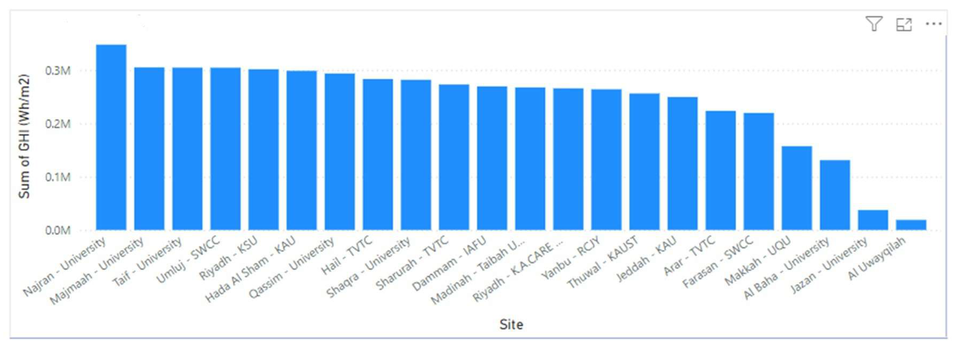
Bar Charts: Bar chart showing average GHI for different sites to identify the most productive locations. Monthly Average GHI: Bar chart to compare average GHI values across different months.
Figure 4.
GHI over different sites, over the years
Figure 4.
GHI over different sites, over the years
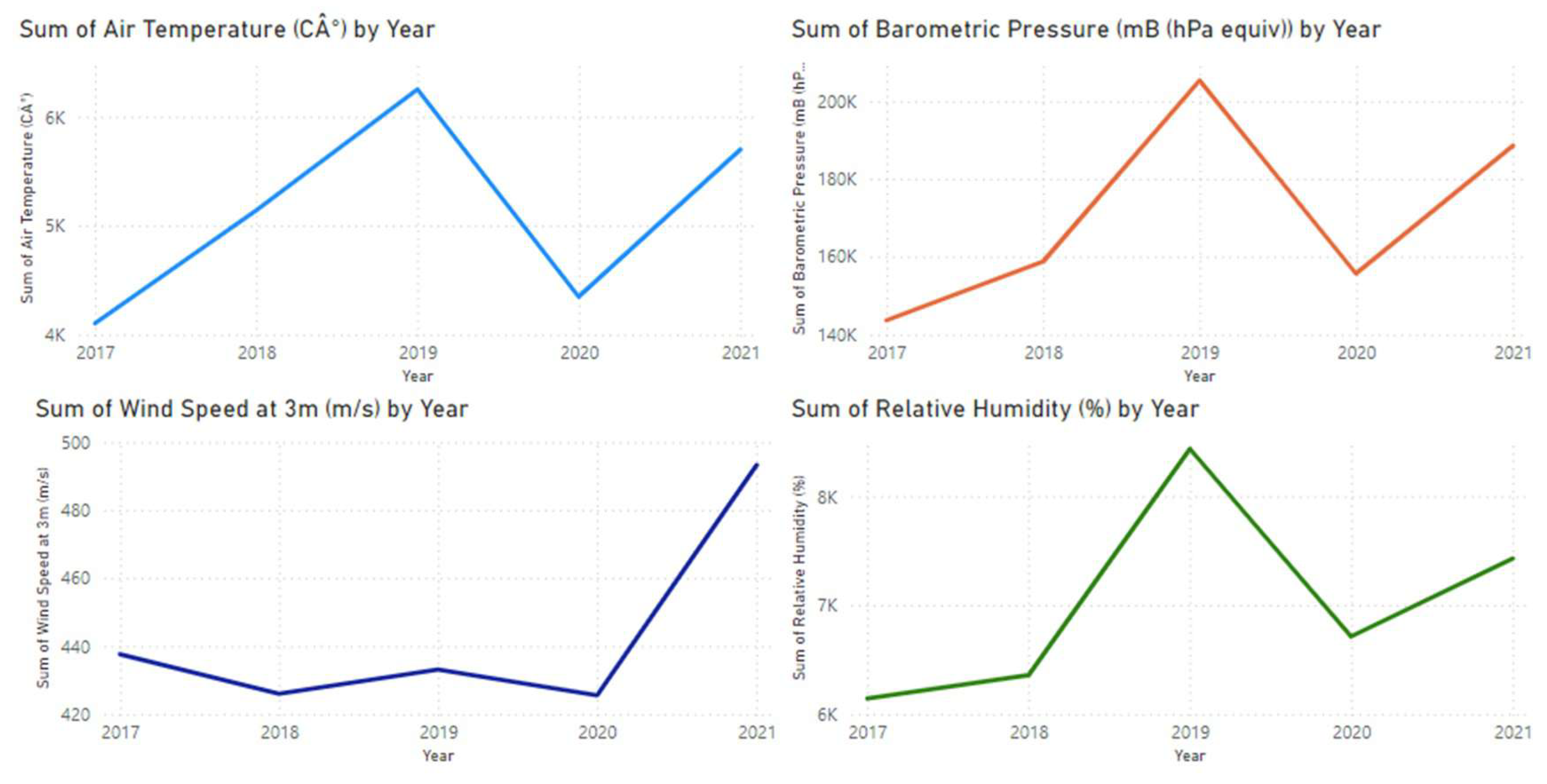
Line Plots: Line plot to compare DHI, DNI, and GHI values over time.
Figure 5.
Variations of meterological parameters, over the years
Figure 5.
Variations of meterological parameters, over the years
The machine learning techniques are then put into practice by writing a Python script. The script provides an integrated data analytic component that is first tested independently on a Jupyter notebook before being integrated into the application architecture. The system is expanded and the visuals and analytical results are reintegrated into visualizations.
At this point, the model is assessed using the case study data set, and metrics like mean average errors, values, confusion matrix, and prediction accuracy. The findings of the empirical tests are then presented in PDF reports and a visual dashboard.
4. The Model Construction
Model construction involves a typical sequence of steps starting from Data preparation, data preprocessing, feature selection, algorithm choice, algorithm implementation, model parameter setting, data splitting, Training and testing, model training, Model evaluation, and predictive visualization.
Given the schema of the data set, the random forest regressor algorithm is chosen for several strong reasons listed below:
Data Variability: The solar data in this case is meteorological data. There can be a lot of variation and noise in meteorological data. Random forest regressor mitigates and optimizes these variations by constructing multiple decision trees. It aggregates the individual results, aiding in reduced unpredictability and reliable forecasts.
Complex correlations: Several variables, including air temperature, wind speed, humidity, and barometric pressure, have complex and non-linear correlations. that affect the production of solar electricity. These relationships can be captured well by Random Forest.
Feature Interaction: It is crucial to consider how different features interact, such as how air temperature and wind speed jointly impact the production of solar electricity. These interactions are naturally captured by Random Forest during the tree-building process.
Apart from these reasons, the random forest regressor is robust, resilient to outliers, and capable of handling both numerical and categorical data well.
4.1. The Random Forest Regressor
A forest as known, is a collection of trees. The random forest here too is a collection of multiple decision trees. It works on the principle of optimized estimation of the predictions of each decision tree inside the forest. This process reduces the risk of over fitting, which is a common issue with individual decision trees. The following
Figure 3 gives an intuitive understanding of the algorithm [
5].
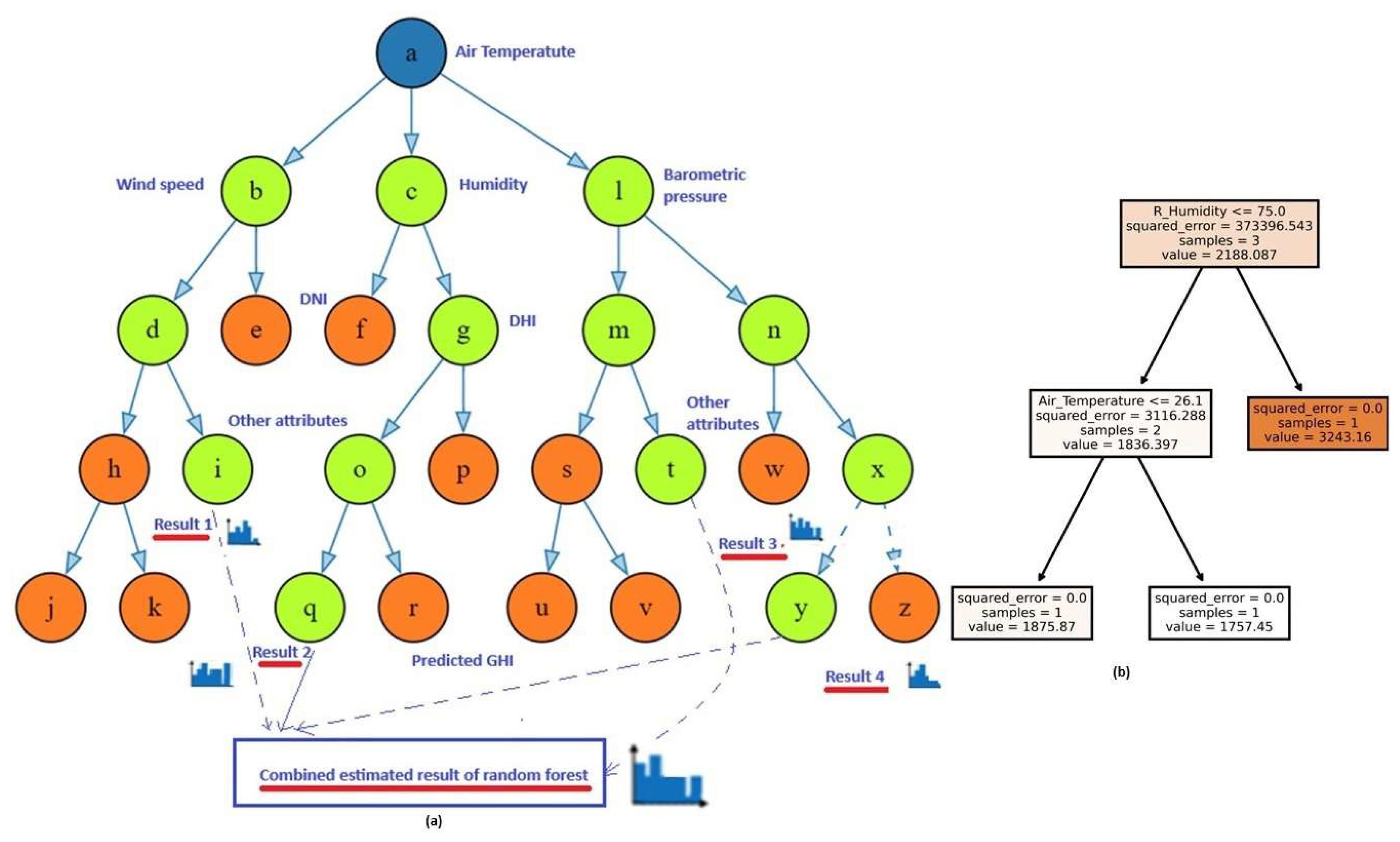
The algorithm generates several decision trees, based on the data set and decision variables. It makes prediction results on each tree. The final prediction of the random forest is computed by taking the optimal best from this pool of individual tree predictions.The green colored nodes indicate decision paths leading to the prediction, the end node of the path. See
Figure 6 (a).
In the context of the schema of solar energy data set and subsequent training, the random forest regressor learns to build an estimator to predict the output. The supervisory learning model for the given data set maps as below:
Input samples are given as an array of shape (n. samples, n. features) E.g. feature values of the solar data set here are:
[ Latitude, Longitude, Date, Air Temperature, Wind Speed, DH, DNI, RH, BP, GHI ]
E.g. The output sample is an array of shape (n. samples,)
The goal of the regressor is to build an estimator for the given dataset such that in the predicted values the error is minimized. The estimator builds a forest of decision trees and estimates the final value by combining individual results of each tree. The estimated error is given by Equation (
Section 4.1) as in [
5].
Where, L is a learning parameter.
Implementing the core logic of machine learning algorithms is simplified by [
19,
20] and [
21].
rf = RandomForestRegressor(random_state=42)
gb = GradientBoostingRegressor(random_state=42)
are the functions for the two algorithms, random forest regressor and gradient boosting respectively. The code prototype for proof of concept is developed using Python [
19]. These scripts are integrated inside the power BI to form an analytic dashboard.
Figure 7 shows the instance of random forest (5 trees) for the illustrative data (X) given above.
The regressor builds a forest of such trees for the given data and estimates the optimal predicted outcome considering the prediction of each tree in the forest. In
Figure 6 (a) shows the intuitive diagram in which dashed lines show the decision paths.
Figure 6 (b) shows a sample tree for the sample data "X" above.
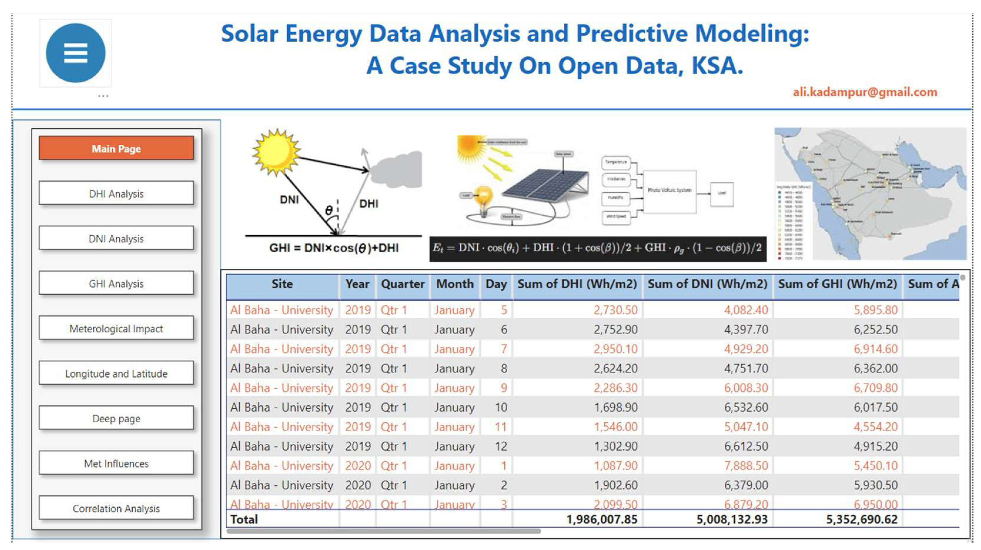
The predictive algorithm is scripted and embedded inside Power BI, as part of the analytic dashboard. The instance of the dashboard is shown in
Figure 8.
5. The Analytic Dashboard
The dashboard has provisions to visualize various analytic outputs with the help of button clicks.
Figure 8 shows the buttons and the main page of the dashboard. The main goal is to study the impact of meteorological parameters on solar energy production. The corresponding analytic results are discussed in the following sections.
6. Results & Discussion
In this section, instances of dashboard, results of correlation analysis, impact of meteorological parameters,predictive analysis, and metric values are presented.
6.1. Correlation analysis
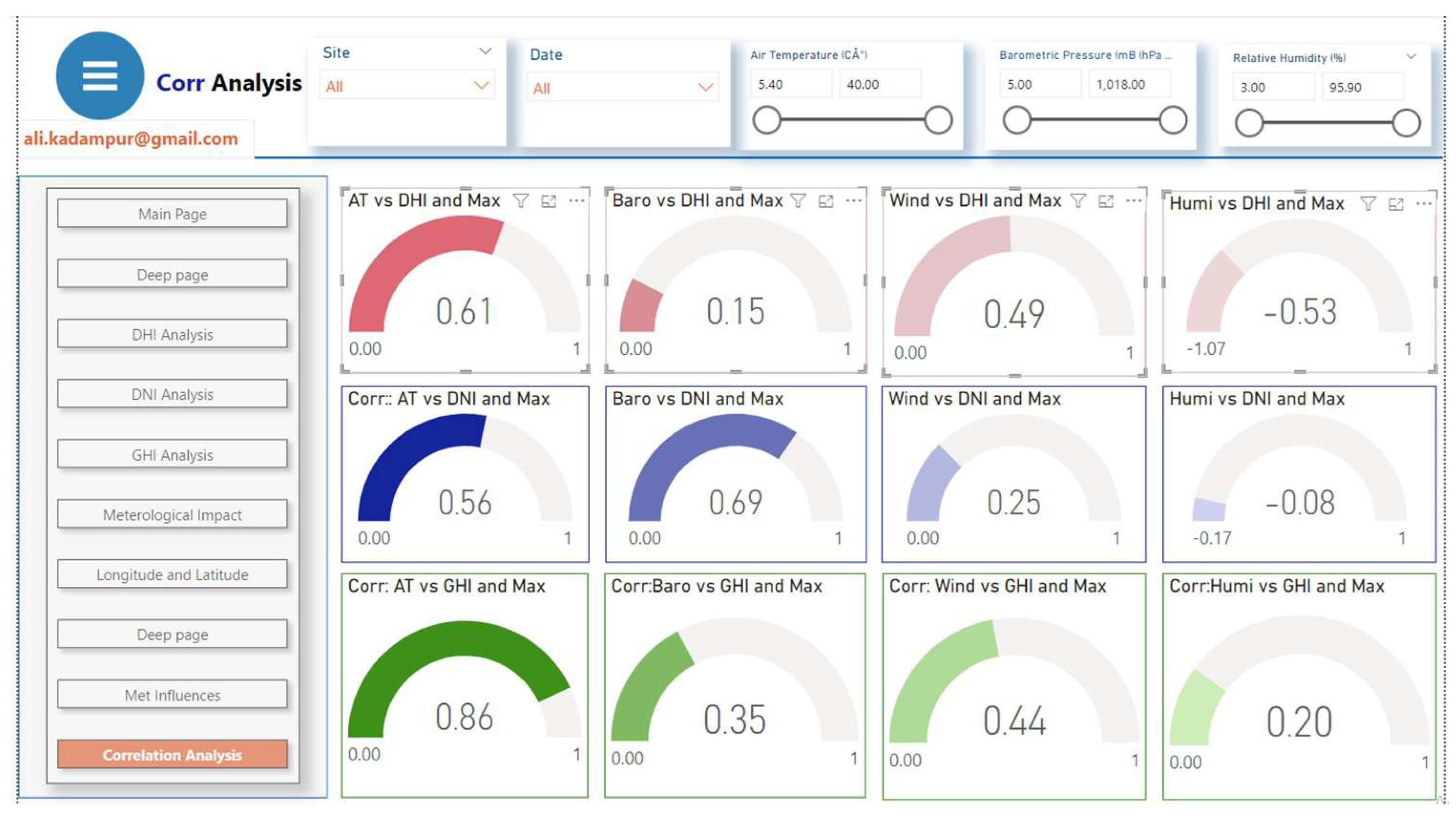
The
Figure 9 shows different correlation values.
Correlation coefficients range from -1 to 1 and indicate the strength and direction of the linear relationship between the two variables. A Positive Correlation Coefficient indicates that one variable increases when the other variable increases. Conversely, a negative correlation coefficient indicates that one variable is increasing while the other is decreasing. The correlation coefficient value of zero indicates that the two variables are not correlated. It is to be noted that the correlation coefficient does not represent the cause and effect relationship between the variables; rather, it only shows the linear relationship between the variables.
Table 2 summarizes the analysis.
6.2. Impact of Meteorological Variables
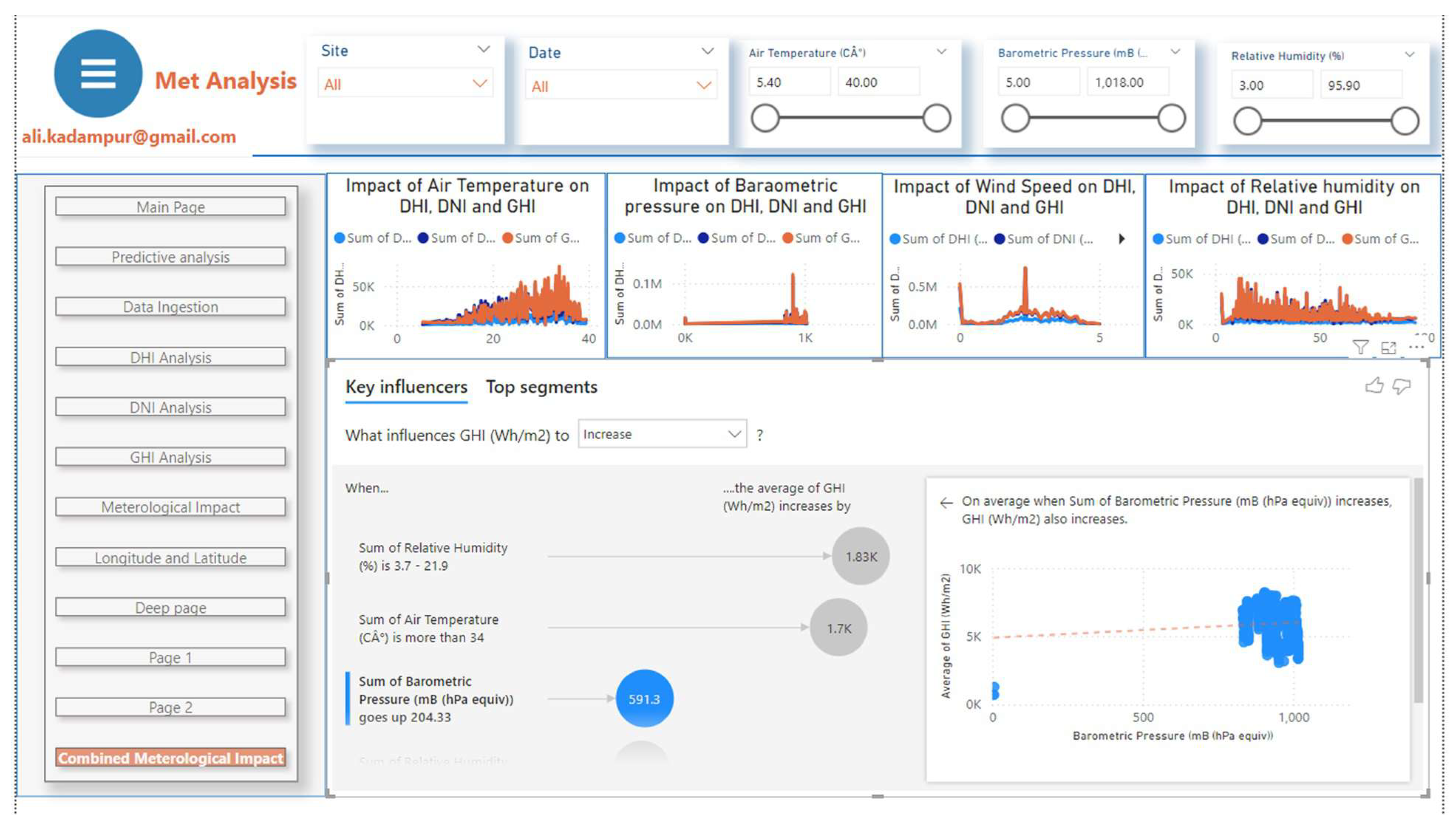
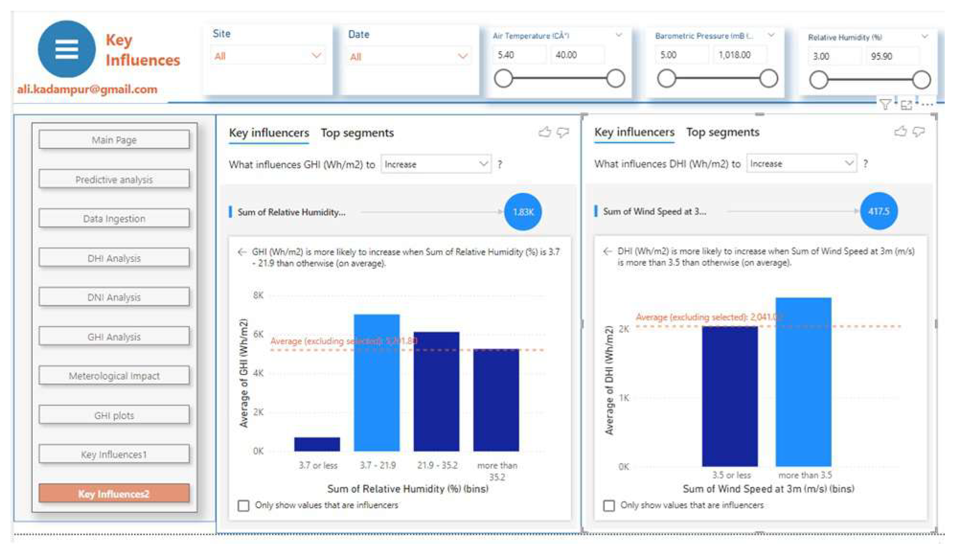
In this section impact analysis of meteorological parameters is carried out by using built in machine learning algorithms of the analytical platform. The visualization feature "Key influencers" of Power BI is applied to get the results. Following
Figure 10 shows the dashboard instance of this analytic output.
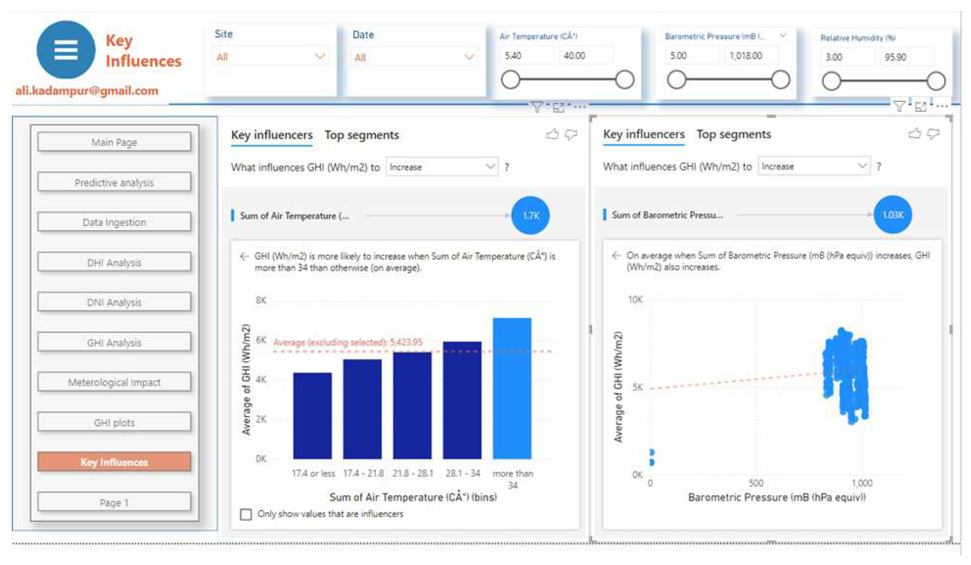
Figure 11,
Figure 12 and the
Table 3 summarize the results of this section.
GHI is more likely to increase when Air Temperature is more than
C, and increase in Barometric Pressure has positive effect on GHI. The GHI increases as Barometric Pressure increases, see
Figure 11. Wind speed has no influence on GHI but it has influence on DHI. DHI increases when WS > 3.5 (m/s), see
Figure 12. GHI is more likely to increase when relative humidity is between 3.7 mB to 21.9 mB See
Figure 12 .The influence of meteorological parameters are summarized in
Table 3
6.3. Predictive Analytics
In this section the prediction results of the random forest regressor and its evaluation metrics are presented.
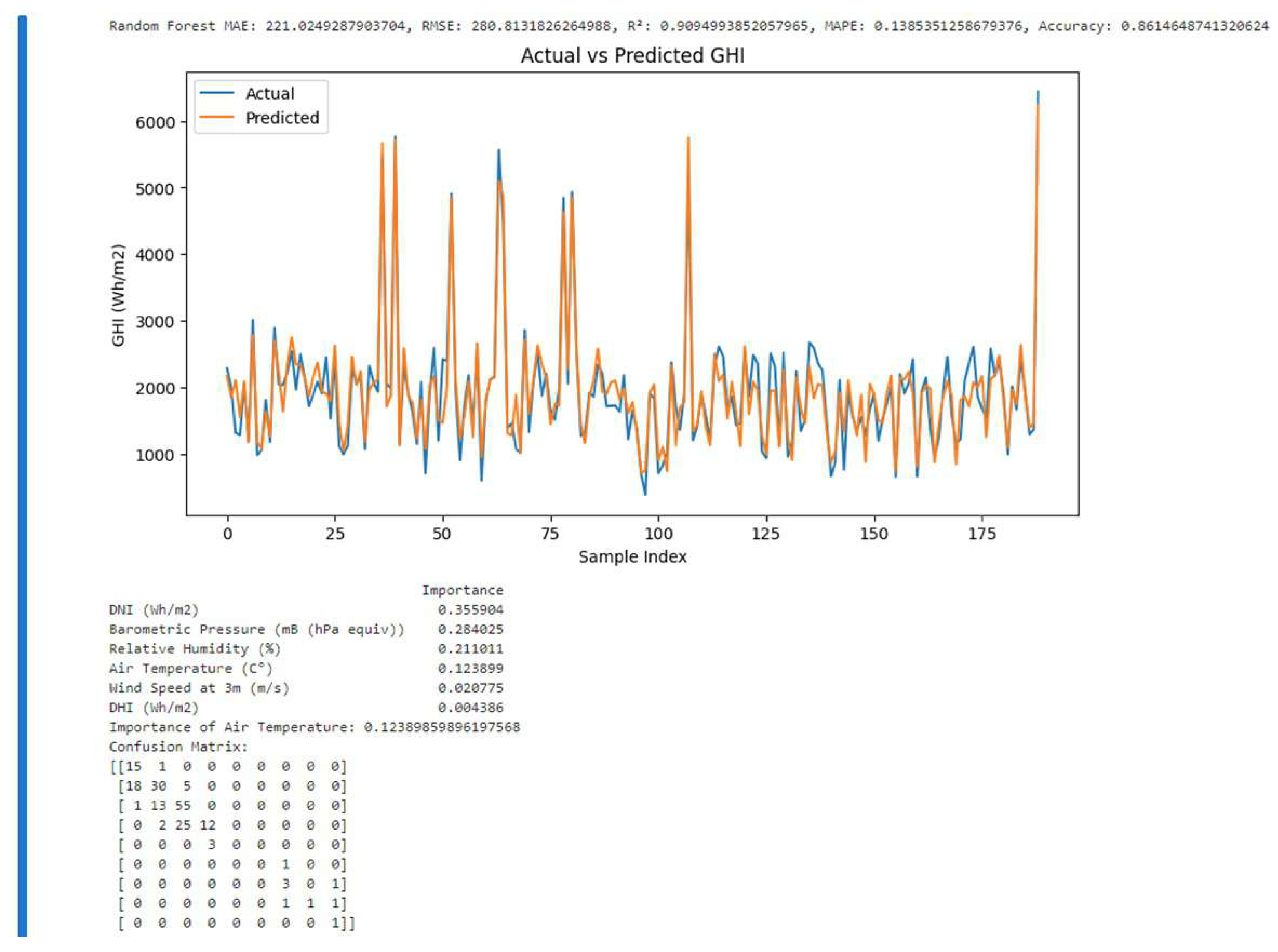
Figure 13 shows the actual GHI values vs Predicted GHI values. This plot shows the meteorological coefficients, the regressor metrics and confusion matrix. The metric values are as follows:
; ;
The MAE of 221.0294 indicates that, on average, the model’s predictions of Global Horizontal Irradiance (GHI) deviate from the actual values by about 221.03 Wh/
The RMSE of 280.81318 suggests a moderate level of error when predicting GHI. RMSE is more sensitive to larger errors compared to MAE.
The value of 0.909499385 indicates that approximately 90.95% of the variance in the GHI data is explained by the model.
Figure 13.
Actual vs Predicted GHI & Metrics:An instance of Predictive Analysis
Figure 13.
Actual vs Predicted GHI & Metrics:An instance of Predictive Analysis
6.4. Model Coefficients & GHI Estimation
The two GHI model estimations are discussed in this section.
In terms of these parameters the multi linear GHI estimator is Equation (
2)
Using the multi linear model coefficients of
Table 4 & Equation (
2), the GHI (multi linear) is computed. The plot in
Figure 15 (a) shows the actual GHI vs the computed GHI over the years. It is observed that the multi linear model, though provides actual GHI values at some instances, it fails to follow the pattern of actual GHI. Arguably, since GHI has complex nonlinear dependency on the meteorological parameters a multi linear equation may be too simple to fit to the model. Therefore, a nonlinear model is required to compute GHI.
Figure 14.
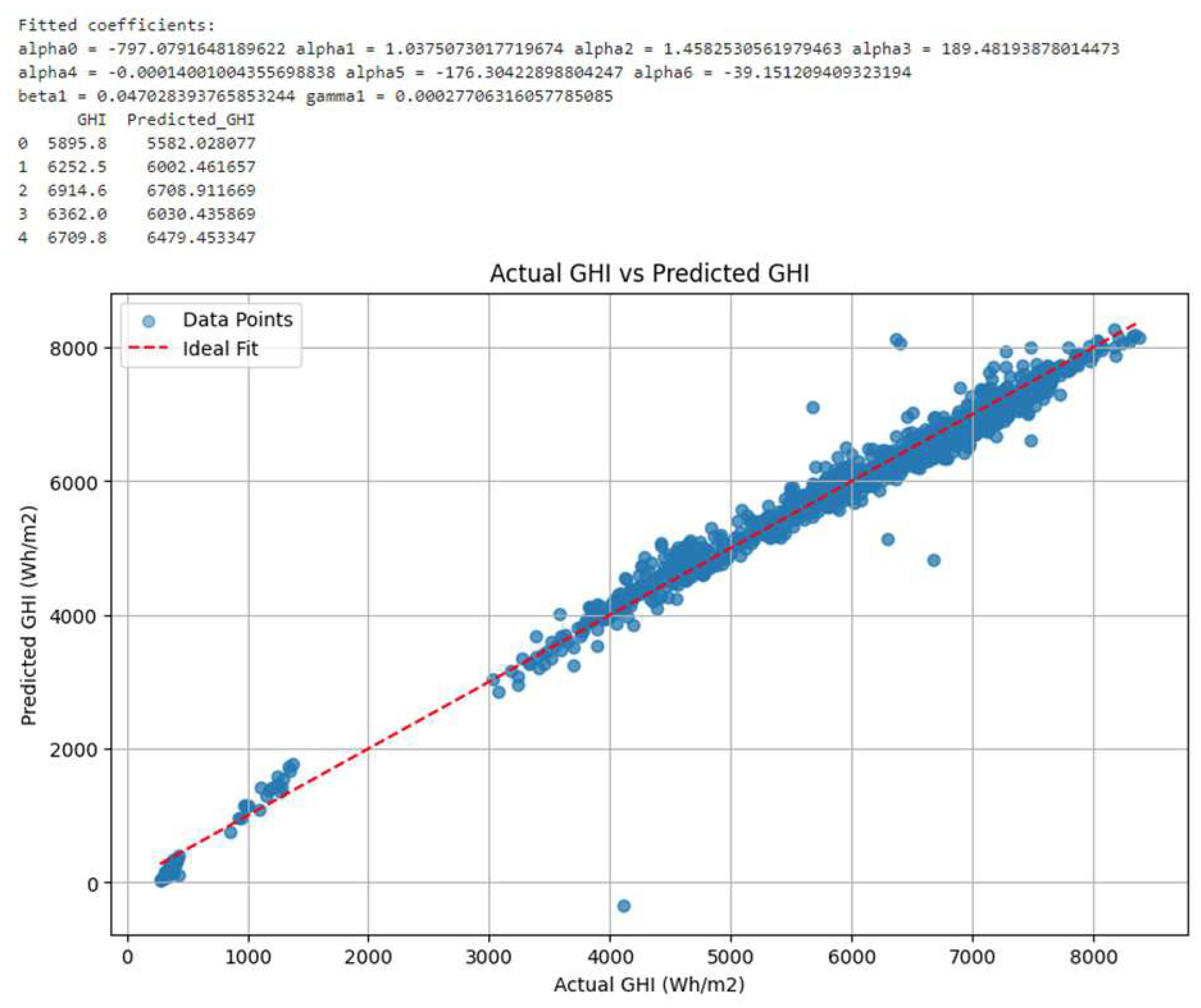
Scatter plot of Actual vs Predicted GHI after Non-linear modeling
Figure 14.
Scatter plot of Actual vs Predicted GHI after Non-linear modeling
Figure 15.
Line graphs of actual and computed GHI under multilinear (a) and Nonlinear (b) modeling
Figure 15.
Line graphs of actual and computed GHI under multilinear (a) and Nonlinear (b) modeling
The Equation (
3) provides a GHI estimation considering the nonlinear dependency on the meteorological paraders.
Figure 14, shows the meteorological model coefficients under nonlinear modeling.
Using these model coefficients and a nonlinear Equation (
3), GHI (Nonlinear) is computed. The plot in
Figure 15 (b) shows the actual GHI vs the computed GHI over the years. It can be noted that the nonlinear model follows the exact pattern as the actual GHI line. The value difference can be compensated by clamping the parameter
. The plot in
Figure 16 (d & e), shows the actual and computed GHI plots under nonlinear modeling. In conclusion of this discussion, Equation (
3) is a better fit for predicting GHI.
Therefore, to estimate GHI in Saudi Arabia, the nonlinear Equation (
3) with the coefficient values given in
Table 5 may be used.
6.5. Confusion Matrix
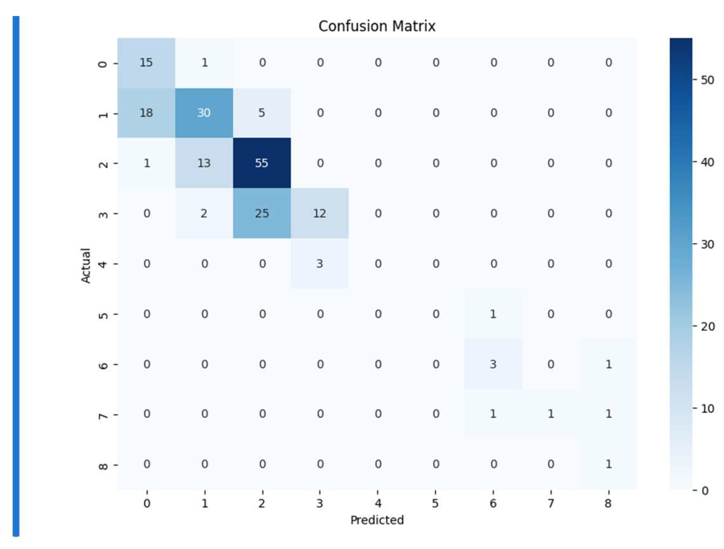
A confusion matrix is a performance measurement tool for machine learning classification algorithms. It is a table that has actual values as rows and predicted values as columns. A multi class classifier may have many columns otherwise it is always a 2x2 matrix. The confusion matrix allows visualization of the performance of an algorithm by comparing the actual target values with the predicted values produced by the model. It benchmarks the confusion factor in the classifier. The colored version of it is called heat map.
Figure 17, shows the heat map obtained for the random forest regressor. A bin size of 10 was initialized to get 10 classes (10x10) in the matrix. Inferences are drawn by comparing the heat map of
Figure 17, with the heat map axioms of
Table 6
Therefore, the inferences drawn from the confusion matrix indicate that the model is performing well.
7. Conclusion & Future Work
In the context of Saudi Arabia’s solar energy production, this study emphasizes the significant influence of meteorological variables on solar power generation. The study successfully illustrates the use of machine learning algorithms, specifically RandomForestRegressor, in the prediction of Global Horizontal Irradiance (GHI) using publicly available meteorological data.
This study highlights the substantial impact of meteorological variables on solar power generation, specifically in the context of Saudi Arabia’s solar energy production. Utilizing open meteorological data, the research effectively demonstrates the application of machine learning algorithms, particularly RandomForestRegressor, in predicting Global Horizontal Irradiance (GHI). Key findings indicate that solar energy production is optimal at barometric pressure levels between 800-1000 mB, and GHI increases significantly when the atmospheric temperature exceeds 34°C. Additionally, lower relative humidity correlates with higher solar energy output, while wind speeds between 2 to 4 m/s, peaking at 2.4 m/s, also positively influence solar power production. The predictive models developed in this study achieved high accuracy, with Random Forest and Gradient Boosting showing R² scores of 0.909499385 and 0.865, respectively. The model has MAE of 221.025, and RMSE of 280.813.These results underscore the efficacy of machine learning in enhancing the accuracy of solar energy forecasts, which is critical for energy management and planning. The paper explored the meteorological coefficients generated by the model and applied them to form a multi-linear equation to compute GHI. The paper identified the short comings of this multi-linear equation and improved the GHI forecasting equation by considering the non-linear coefficients. Equation (
3) with parameters of
Table 5 is an important outcome of this research to compute GHI in Saudi Arabian context.
The paper integrated machine learning models into Power BI and demonstrated the practical application of data analytics and visualization tools in renewable energy. This approach not only facilitates better understanding and optimization of solar energy production but also supports the broader goal of integrating renewable sources into the energy grid.
Future research has scope for improvement. It can be said that the outcome of machine learning algorithms is as good as the data used. In this case study, the open data was found to be limited in terms of monthly span and number of records in each location.If the data collection authorities pay attention to update this data, the research in this area will be greatly benefited. Based on the findings in this paper the work can expand to incorporating additional features and exploring other machine learning techniques to further refine prediction models and enhance solar energy forecasting accuracy.
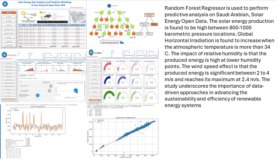
The study underscores the importance of data-driven approaches in advancing the sustainability and efficiency of renewable energy systems.
Funding
This work was supported and funded by the Deanship of Scientific Research at Imam Mohammad Ibn Saud Islamic University (IMSIU) (grant number IMSIU-RG23155).
Data Availability Statement
The Open Data sets are available at
Open Data.The preprocessed data along with the dashboard is available at github repository and the personal website at
myGithub &
DrMAK School.
Acknowledgments
I would like to thank, the Deanship of Research & Development, Imam Mohammad Ibn Saud Islamic University, Riyadh, KSA for encouraging to work on renewable energy particularly AI & Predictive analytics applications to Solar energy. Thanks are due for the Open Data initiative of government of Saudi Arabia.
Conflicts of Interest
The author declares no conflicts of interest.
Abbreviations
The following abbreviations are used in this manuscript:
| AI |
Artificial Intelligence |
| AT |
Air Temperature |
| BI |
Business Intelligence |
| BP |
Barometric Pressure |
| DHI |
Direct Horizontal Irradiation |
| DNI |
Direct Normal Irradiation |
| GHI |
Global Horizontal Irradiation |
| H |
Relative Humidity |
| IEA |
International Energy Agency |
| IoT |
Internet of Things |
| KSA |
Kingdom of Saudi Arabia |
| mB |
Millibars |
| ML |
Machine Learning |
| OGD |
Open Government Data |
| P |
Barometric Pressure |
| PV |
Photo Voltaics |
| RH |
Relative Humidity |
| RFA |
Random Forest Algorithm |
| RFR |
Random Forest Regressor |
| T |
Air Temperature |
| URL |
Uniform Resource Locator |
| W |
Wind Speed |
| WS |
Wind Speed |
| XGBoost |
Extreme Gradient Boost |
References
- Halliday, D.; Resnick, R.; & Walker, J.Fundamentals of Physics; 10th Eds.; Wiley & Sons: Danvers, Massachusetts, USA, 2010; pp. 195.
- REN21:Renewable Energy Now. Available online: URL https://www.ren21.net/reports/global-status-report/ (accessed on 07/10/2024).
- Renewables. Available online: URL https://www.iea.org/reports/renewables(accessed on 07/10/2024).
- Adnan Ayaz.;Faraz Ahmad.;Mohammad Abdul Aziz Irfan.;Zabdur Rehman.;Krzysztof Rajski.; and Jan Danielewicz. Comparison of Ground-Based Global Horizontal Irradiance and Direct Normal Irradiance with Satellite-Based SUNY Model. Energies 2022, 15(7), 2528. [CrossRef]
- Breiman, L. Random Forests. Machine Learning 2001, 45, 5–32. [Google Scholar] [CrossRef]
- Ali Jassim M Lari. Forecasting and Prediction of Solar Energy Generation using Machine Learning Techniques. Doctor of Philosophy, Swansea University, Wales UK, 20/06/2023.
- Ewa Chodakowska.; Joanicjusz Nazarko.; Lukasz Nazarko.; and Hesham S. Rabayah. Solar Radiation Forecasting: A Systematic Meta-Review of Current Methods and Emerging Trends. Energies 2024, 17(13), 3156. [CrossRef]
- Yang D.; Kleissl, J.; Gueymard C. A.; Pedro H. T. C.; & Coimbra C. F. M. History and trends in solar irradiance and PV power forecasting: A preliminary assessment and review using text mining. Solar Energy 2018, 168, 160–101. [CrossRef]
- Huijun Zhang.; Mingjie Zhang.; Ran Yi.; Yaxin Liu.; Qiuzi Han Wen.; and Xin Meng. Growing Importance of Micro-Meteorology in the New Power System: Review, Analysis and Case Study. Energies 2024, 17(6), 1365. [CrossRef]
- Chen C.; Liaw A.; & Breiman L. (University of California, Berkeley. USA); 2004.
- Geurts P.; Ernst D.; & Wehenkel L.Extremely randomized trees. Machne Learning 2006, 63, 3–42. [CrossRef]
- Lingjun He.; Richard A.; Levine.; Juanjuan Fan.; Joshua Beemer.; Jeanne Stronach. Random Forest as a Predictive Analytics Alternative to Regression in Institutional Research Practical Assessment, Research & Evaluation Journal 2018, 23(1), 1–16. ISSN:1531-7714.
- Rob Kitchin.The Data Revolution: A Critical Analysis of Big Data, Open Data and Data Infrastructures; 2nd Eds.; SAGE: Oliver’s Street, London, UK, 2022; pp. 43-75. ISBN:978-1529733754.
- Arie Purwanto.; Anneke Zuiderwijk.; and Marijn Janssen. Authors Info & Claims "Citizens’ Trust in Open Government Data: A Quantitative Study about the Effects of Data Quality, System Quality and Service Quality. In Proceedings of 21st Annual International Conference on Digital Government Research, Seol, Republic of Korea, (15-19/06/2020); Pages 310–318. [CrossRef]
- Cong Feng.; Dazhi Yang.; Bri-Mathias Hodge.; Jie Zhang. OpenSolar: Promoting the openness and accessibility of diverse public solar datasets. Solar Energy 2019, 188(1), 1369–1379. [CrossRef]
- Aneela Zameer.; Fatima Jaffar.; Farah Shahid.; Muhammad Muneeb.; Rizwan Khan.; Rubina Nasir. Short-term solar energy forecasting: Integrated computational intelligence of LSTMs and GRU PLoS ONE 2023, 18(10): e0285410. [CrossRef]
- Stefan Preda.; Simona-Vasilica Opre.; Adela Bâra.; and Anda Belciu (Velicanu). PV Forecasting Using Support Vector Machine Learning in a Big Data Analytics Context. Symmetry 2018, 10(12), 748. [CrossRef]
- Giheung-gu.; Yongin-si.; Gyenggi-do. A Two-Step Approach to Solar Power Generation Prediction Based on Weather Data Using Machine Learning. Sustainability 2019, 11(5), 1501. [CrossRef]
- Andreas C. Müller.; and Sarah Guido. Introduction to Machine Learning with Python.; Oreilly publisher: Gravenstein Highway North, Sebastopol, CA, USA. 2017; pp. 378. ISBN:978-1-449-36941-5.
- Pedregosa F.; Varoquaux G.; Gramfort, A.; Michel, V.; Thirion, B.; Grisel O.; & Duchesnay, E. Scikit-learn: Machine Learning in Python. Journal of Machine Learning Research 2011, 12, 2825–2830.
- Annie Leung.; & Janni Leung. (University of Queensland, Queensland. UK). "How to use Python in Power BI? Step-by-step tutorial – a case study of creating a correlation heatmap, 2020. [CrossRef]
|
Disclaimer/Publisher’s Note: The statements, opinions and data contained in all publications are solely those of the individual author(s) and contributor(s) and not of MDPI and/or the editor(s). MDPI and/or the editor(s) disclaim responsibility for any injury to people or property resulting from any ideas, methods, instructions or products referred to in the content. |
© 2024 by the authors. Licensee MDPI, Basel, Switzerland. This article is an open access article distributed under the terms and conditions of the Creative Commons Attribution (CC BY) license (http://creativecommons.org/licenses/by/4.0/).
