Preprint
Article

Hydropower Plant Available Energy Forecasting Using Artificial Neural Network and Particle Swarm Optimization

Altmetrics

Downloads

119

Views

38

Comments

0

A peer-reviewed article of this preprint also exists.

This version is not peer-reviewed

Submitted:

21 July 2024

Posted:

25 July 2024

You are already at the latest version

Alerts
Abstract
Accurate forecasting of available energy portion that corresponds to the reservoir inflow of the month(s) ahead provides important decision support for the hydropower plants in energy pro-duction planning for revenue maximization, as well as for the environmental impact prevention, and flood control at the upstream and downstream of a basin. Therefore, a reliable forecasting tool or model is deemed necessary and crucial. Considering the fluctuation and nonlinearity of data which significantly influence the forecasting results, this study develops an effective hybrid model by integrating Artificial Neural Network (ANN) and Particle Swarm Optimization (PSO) called “PSO-ANN” model based on the hydrological and meteorological data pre-processed by cross-correlation function (CCF), autocorrelation function (AFC), and normalization techniques for predicting the available energy portion corresponding to the reservoir inflow mentioned above for a case study hydropower plant in Laos namely, Theun-Hinboun hydropower plant (THHP). The model was evaluated by using correlation coefficient (r), relative error (RE), root mean square error (RMSE), and Taylor diagram plots in comparison with the popular single algorithm approaches such as ANN, and NARX models. Results demonstrated the superiority of the proposed PSO-ANN approach over the other two models.
Keywords: 
Subject: Engineering  -   Electrical and Electronic Engineering

1. Introduction

At present, renewable energy (RE) plays a crucial role in a clean energy supply in which one of the significant sources of RE is hydropower [1]. In a hydropower plant, accurate forecasting of available energy or reservoir inflow is necessary for ensuring optimal operation of the reservoir as sufficient water needs to be maintained in the reservoir in the dry season while unplanned or unreasonable spillage needs to be avoided in the wet season. The optimal reservoir operation is directly associated with generation planning that supports revenue maximization, as well as environmental impact prevention, and flood control at the upstream and downstream of a basin [2]. Due to real hydrological and meteorological data having the characteristics of fluctuation and nonlinearity resulting from the extensive influence of human activity and natural factors [3]; several studies have given more attention to the methodology of high precision forecasting of which two fundamental techniques for forecasting, physically based and data-driven models, are widely implemented [4]. The results provided by the physically based models are more explainable compared to those of data-driven models [5]. The existing physically based models including, but not limited to CalSim, WEAP, and HEC ResSim are regarded as powerful tools for forecasting as they are based on the principles of mass and hydrological conservation, and the laws of physics [6]; however, these physical models had some limitations resulting from their requirements for a huge effort in terms of hydrological and climate data, and time-consuming in the learning process [7]. Therefore, the data-driven approaches are the alternative solutions as these approaches are highly adaptable and able to be constantly optimized and updated hence, promising accurate forecasting [8].
In the past decades, The data-driven methods with a single algorithm have gained a lot of attention as a result of their simplicity such as the Adaptive Neuro-Fuzzy Inference System (ANFIS) model utilized for monthly dam inflow prediction in which the model with three input variables i.e. monthly rainfall, dam inflow and rainfall forecast of next month provided a higher accuracy than the other models [9]; Recurrent Neural Network (RNN) based on radar rainfall data and reservoir inflow data for multi-step-ahead reservoir inflow forecasting outperformed the Back Propagation Neural Network (FFBPNN) [10]; multi-layer perceptron (MLP) artificial neural network model for one-month-ahead inflow forecasting for the Ubonratana reservoir situated in Thailand revealed the better performance of the Type F (with inflow known and assumed to be the forecast) model over the other models [11]; Support Vector Machine (SVM) models considered different monthly time lags for predicting inflow to Zayandehroud dam reservoir in Iran displayed more accurate results than those of the ANN models [12]; Bayesian Networks (BN) model for annual and monthly inflow forecasting for the Zayandehrud dam reservoir in Iran depicted a more reliability over the other limited research conducted in the study area [13]; Nonlinear Auto-Regressive with exogenous input (NARX) model, and Nonlinear Auto-Regressive (NAR) model provided good alternative approaches for inflow forecasting such as the forecast for a case study reservoir in Iran (Sefidruod dam reservoir) which depicted a capability of the NAR model over the NARX [14]; hydropower generation prediction using SVM, ANN and ARIMA for three Gorges Dam situated in China demonstrated the superiority of the ANN model over the other models with the correlation coefficient (r) between 0.9011 and 0.8883 [15]. After reviewing the literature, some limitations of the single technique were detected such as overfitting of ANN, parameter uncertainty of SVM, local minimization drawback of PSO, cognitive uncertainties of Fuzzy logic, and lack of memory in genetic programming [16] especially when employed for the fluctuation and nonstationary data of different hydrological and climatic conditions thus influenced the forecasting accuracy; hence many researchers developed the hybrid models, instead of the single algorithm models, with the aim of improving the accuracy in the forecasting [8].
A hybrid model of SARIMA–GEP integrated a Seasonal Autoregressive Integrated Moving Average (SARIMA) and the gene expression programming (GEP) carried out for monthly reservoir inflow forecasting provided more accurate forecasting over the single algorithm models like ANN, GEP, and SARIMA models [17]; a DEL-LSTM model combined a Decomposition-Ensemble Learning (DEL) and Long Short Term Memory (LSTM) for predicting daily reservoir inflow outperformed the standalone ARIMA, DNN, MDFL, and LSTM [18]; a Hybrid Deep Learning Inflow Prediction-Rolling Window called “HDeepLIP-RW models” provided superiority over several single algorithm models namely, ANN, RNN, MLR, GRU, and LSTM [19]; a fusion-based model combined several individual artificial neural networks (ANNs) with the moderate-resolution imaging spectroradiometer (MODIS) data increased the accuracy in forecasting monthly reservoir inflow [20]. As an alternative, this study develops effective hybrid models by integrating the Artificial Neural Network (ANN) and Particle Swarm Optimization (PSO) based on the hydrological and meteorological data, properly pre-processed by cross-correlation function (CCF), autocorrelation function (AFC), and normalization techniques, to forecast the available energy portion corresponding to the reservoir inflow mentioned above.
Previously, some researchers adopted a hybrid of Particle Swarm Optimization (PSO) and Artificial Neural Network (ANN) based-models known as “PSO-ANN models” in the forecasting works such as an electrical load prediction in which the PSO algorithm was used for solving the problem related to day-ahead load shifting and the cost saving with demand response (DR) program in combination with the multilayer feed-forward model [21]; a water level prediction by employing the PSO as an optimizer to search for the optimal parameter values for the ANN training process [22]; an application of PSO in optimizing the weights and biases of the ANN to enhance accuracy and performance of the prediction model for gas metering system [23]; a preference prediction in Multi-Criteria Recommender System (a powerful online tools that help to overcome problems of information overload) by training the feed-forward neural networks with the particle swarm optimization (PSO) algorithm and then used the neural network as an aggregation function for predicting the preferences of the users [24]; a behaviour prediction and structural optimization of lightweight sandwich composite heliostats by using the PSO-ANN approach [25]; a crack prediction in pipeline using PSO-ANN whereas the PSO algorithm was employed to enhance ANN training parameters (biases and weights) by minimizing the difference between actual and desired outputs and then using these parameters to generate the network [26]. Based on the aforementioned, we found that the hybrid of ANN and PSO has been employed in several fields of forecasting effectively, except in the reservoir inflow or available energy prediction area, hence this study aims to take advantage of the PSO-ANN approach to forecast the available energy portion corresponding to the Nam Gouang reservoir inflow of the case study hydropower plant in Laos (THHP) which constitutes a novelty approach for the forecasting on this field. To reflect the real application in the commercial hydropower plants and/or the case study hydropower plant as illustrated in Figure 3, this study converted the historical monthly reservoir inflow into the energy unit (available energy in GWh) before the forecasting. By forecasting the available energy portion corresponding to reservoir inflow, the case study hydropower plant can significantly improve its decision support for energy production planning that maximizes revenue. This forecasting also aids in environmental impact prevention and flood control upstream and downstream of the basin. In essence, the hydropower plant will consider the forecasted available energy portion alongside the actual available energy portion, that corresponds to existing water in the reservoir, to determine the amount of energy it can declare for sale in each month ahead. This decision aligns with annual supply targets and ensures sufficient available energy throughout the year. Additionally, this approach helps prevent unreasonable or unplanned reservoir spillage during the wet season, which could lead to lost generation opportunities.
This study has two main goals. The first is to develop the proposed PSO-ANN models in the MATLAB environment. The second is to evaluate the prediction performance of the proposed models using the testing data cluster (not included in the training data cluster), and statistical indicators including correlation coefficient (r), relative error (RE), and root mean square error (RMSE) in couple with Taylor diagrams.
The remainder of this paper is divided into three main Sections. Section 2 introduces the methodology. Section 3 describes the results and discussion. Finally, Section 4 presents the conclusions.

2. Methodology

In this Section, we introduce the research framework of the proposed methodology, which includes the overview of the PSO-ANN concept, comprehensive descriptions of the case study hydropower plant, and data preparation as well as those of the Artificial Neural Network (ANN) and Particle Swarm Optimization (PSO).

2.1. Research Framework

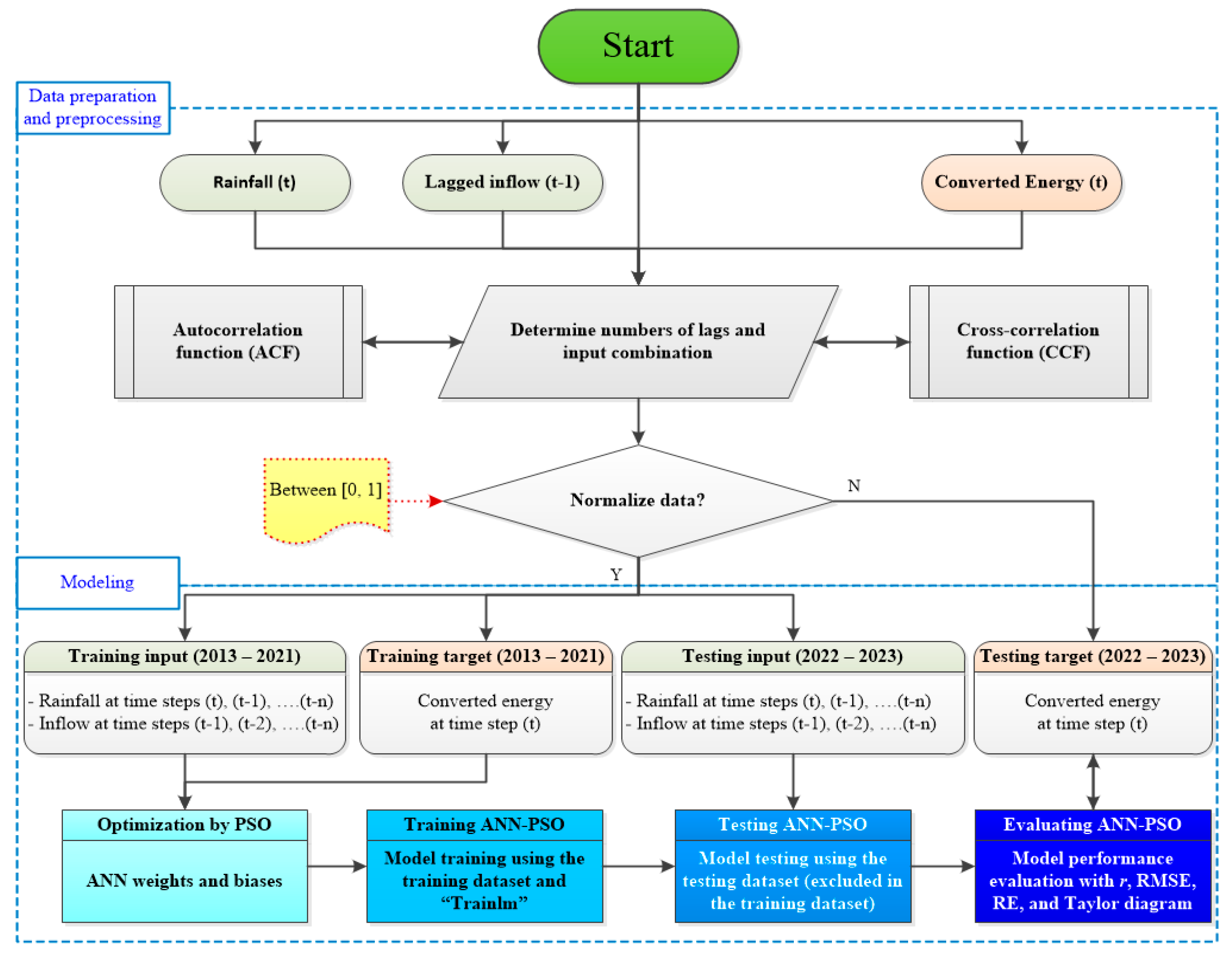
This study was carried out to develop the hybrid models for the forecasting of the month-ahead available energy portion corresponding to the reservoir inflow by integrating the ANN and PSO based on the available historical hydrological and meteorological data of the Nam Guouang reservoir of the Theun-Hinboun hydropower plant, which is the case study hydropower plant situated in Laos, hereinafter referred to as “THHP”. Another goal of this study is to evaluate the performance of the proposed models in comparison with the single algorithm models i.e., ANN, and NARX models. The flowchart of the proposed approach is illustrated in Figure 1. In the data preparation and preprocessing phase, the hydrological and meteorological data including historical monthly rainfall, and inflow data (available in the case study hydropower plant) influencing the prediction results were collected, then the cross-correlation function (CCF) and autocorrelation function (AFC) were employed to determine the number of input lags and combinations for the proposed models. For the achievement of better results and faster learning, the datasets were normalized into numbers between 0 and 1 before plugging into the proposed PSO-ANN models. With respect to the modelling process, four main steps were carried out including (1) optimizing the ANN weights and biases using the PSO algorithm thus obtaining the optimal network, (2) training the models by the “trainlm” function, and using a training cluster (3) testing the trained models by using a separated testing cluster (not included in the training cluster), and (4) evaluating the model by calculating the correlation coefficient (r), relative error (RE), root mean square error (RMSE) in couple with Taylor diagrams.

2.2. Study Area

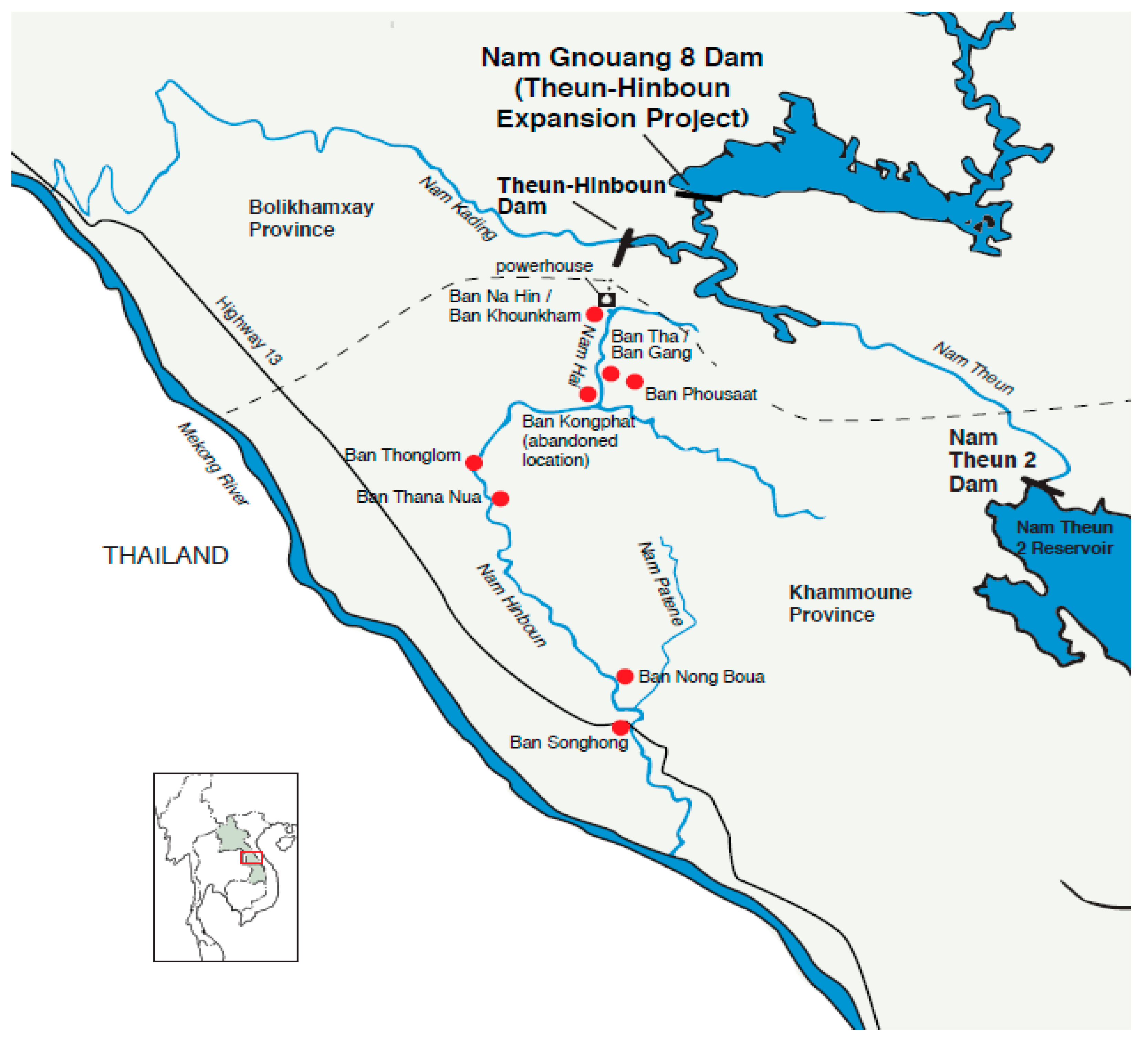
This study implemented the Energy Forecasting for the Theun-Hinboun Hydropower Plant (THHP) situated in the co-area of Khammouane and Bolikhamxay Provinces in Laos approximately 217 km to the east of Vientiane capital and owned by Theun Hinboun Power Company (THPC). Initially, a 220 MW run-of-river project, consisting of two spillway radial gates, a head pond with full supply level of 400 m asl, and generation capacity of 1,100 GWh per year, has been constructed of which 95% of electricity is purchased by the Electricity Generating Authority of Thailand (EGAT). The remaining 5% is for domestic supply to Electricité du Lao (EDL). After the operation for a decade, THPC has expanded the project to a total installed capacity of 500 MW by constructing a new reservoir on the Nam Gnouang River which is a tributary of the mainstream of the existing run-of-river project. The new Nam Gnouang Dam, hereinafter referred to as “NG”, is constructed approximately 20 kilometers upstream of the existing Weir Dam in the form of a concrete gravity Dam with a structure of 480 meters wide and 65 meters high created the NG reservoir with storage capacity of up to 2,430 million cubic meters (MCM) at the full supply level of 455 masl. The NG Dam consists of five spillway gates operated only to discharge water during the wet season to avoid flood event(s). Figure 2
During normal operation, the NG Dam releases water through the NG Powerhouse, which can generate power up to 60 MW for domestic supply to the EDL from the NG Powerhouse. After the NG reservoir, the water flows into the Theun River and the existing head pond above the original Weir Dam. The water finally flows through the new intake and tunnel system to the expanded Theun-Hinboun Powerhouse located approximately 240 meters below in the Na Hin town of Khounkham District. At this location, a new 220 MW Francis generator has been installed alongside the existing two (2) 110 MW generators. After the powerhouse, the water flows to a spillway and then a regulating pound before releasing into the Nam Hai River which is a tributary of the Hinboun River. The new NG reservoir enables THPC to export up to 440 MW to EGAT in which the power is transmitted to a designated delivery point at the Thakhek substation on the Lao PDR-Thailand border via a 230 kV double-circuit transmission line with a total length of approximately 86 kilometers while the remaining 60 MW are allocated for the domestic supply which purchased by the EDL.
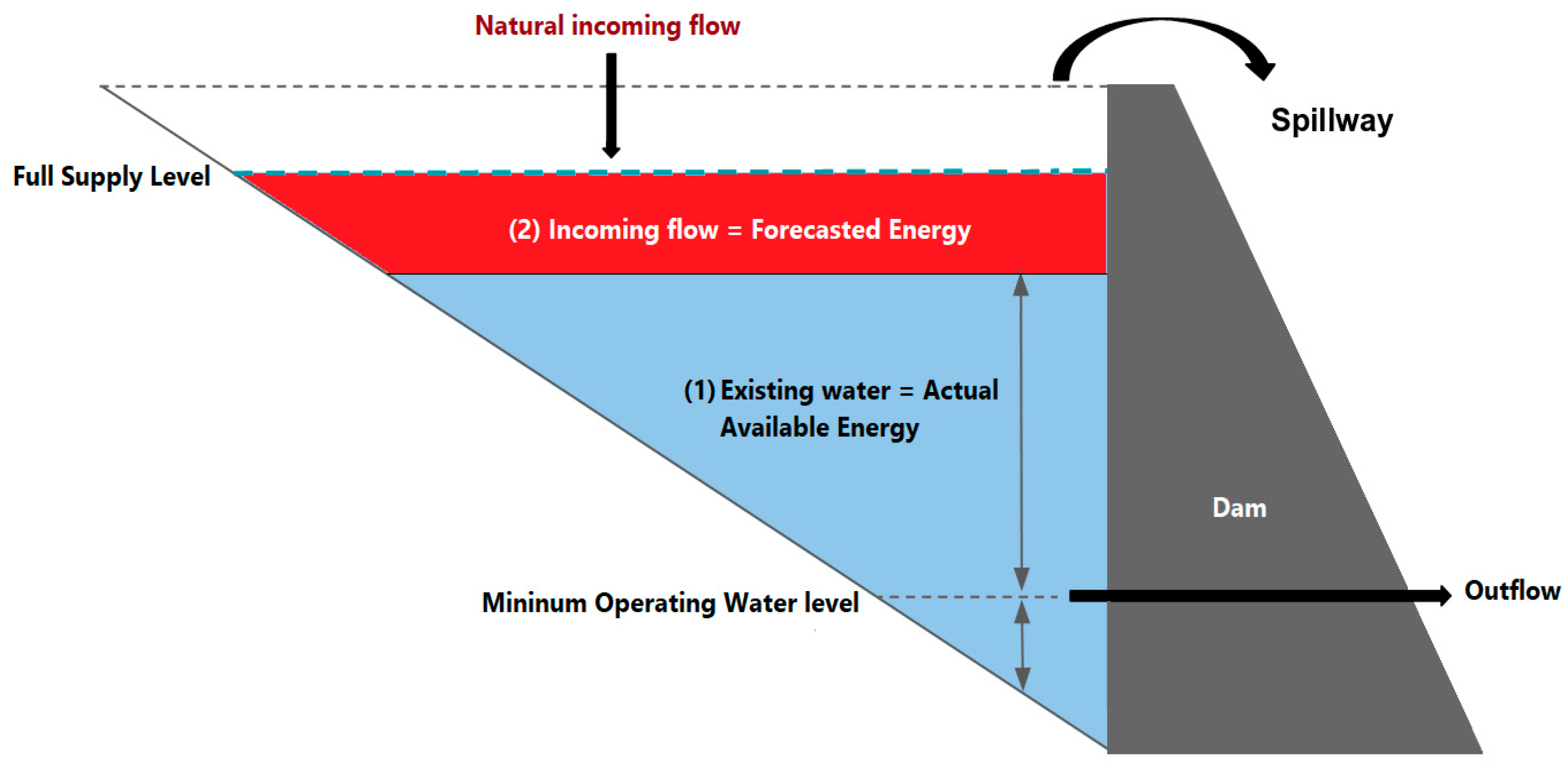
The power purchase agreement between the THPC and EGAT is in the form of the take-or-pay principle with a contract term of 25 years commencing from the commercial operation date (COD). To ensure optimal generation planning associated with revenue maximization as well as environmental impact prevention, and flood control at the upstream and downstream of the basin, the THPC needs to take into account two key energy portions before declaring the energy amount (availability) for selling including the actual available energy portion that corresponds to the existing water in the Nam Gnouang reservoir and head pound at the time of declaration, and the future energy (forecasted energy) that corresponds to the natural inflow (reservoir inflow) expected to flow into the reservoir and head pound in the days and/or months ahead as illustrated in Figure 3.

2.3. Data Preparation

Initially, the historical hydrological and meteorological data including rainfall, and reservoir inflow of the Nam Gnouang reservoir of the THHP were collected from the measurement stations, and some missing data were filled by using the backpropagation technique. The total duration of the data was 11 years (1 January 2013 to 31 December 2023). To reflect the real-world application in the commercial hydropower plants and/or the case study hydropower plant as illustrated in Figure 3, the historical reservoir inflow of the time step (t) has been converted into the energy unit (available energy in GWh) before applying to the models based on the THHP energy coefficient at 0.56117 kWh/m3. The collected data was then analyzed, normalized, and partitioned into four clusters including (i) training input cluster (rainfall and lagged inflows); (ii) training target cluster (converted available energy); (iii) testing input cluster (same parameters of the training input cluster); and (iv) testing target cluster (same parameter of the training target cluster) whereas the duration of the training input cluster and training target clusters were the same at 9 years (approximately 80%) ranging from 1 January 2013 to 31 December 2021, and those of the testing input cluster and testing target clusters at 2 years thereafter (approximately 20%) ranging from 1 January 2022 to 31 December 2023 in compliance with the partition ratio recommended by the previous study [4]. The training input and target clusters were collectively referred to as the “training dataset”, and the testing input and target clusters were collectively referred to as the “testing dataset” in this study.
To determine the number of delays (input time lags) and input combinations for the proposed models, the correlation of every single parameter as well as between each input parameter, and the target parameter were analysed with the autocorrelation function (AFC), and cross-correlation function (CCF). In addition to the data analysis by ACF and CCF, all the data were also normalized into numbers between [0, 1] to ensure faster learning and achievement of better results [27] by using Equation (1):
x ' k = ( x k x min ) ( x max x min )
where x k is the sampling data; x min is the minimum value of the sampling data; and x max is the maximum value of the sampling data.

2.4. Artificial Neural Networks (ANN)

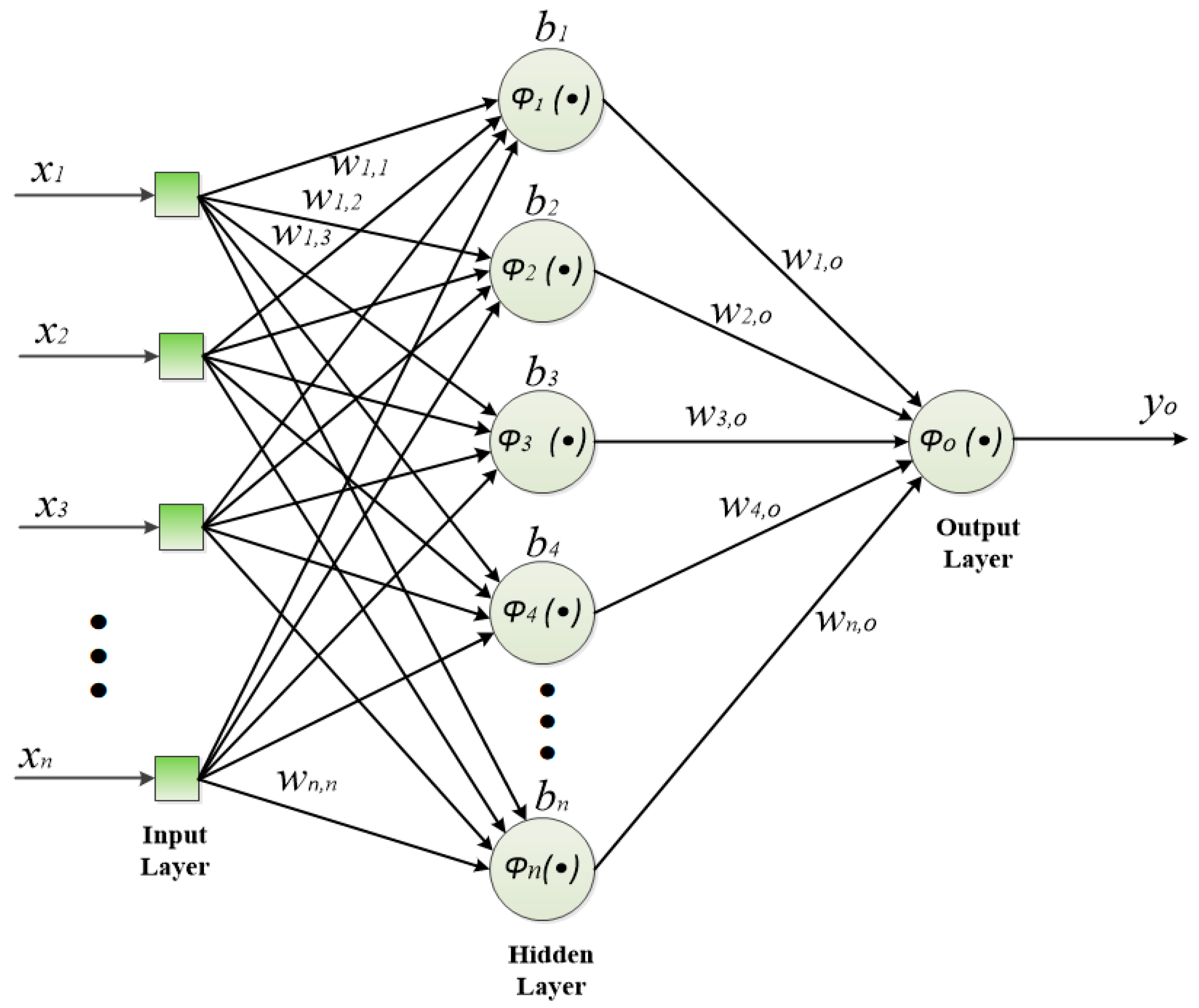
Artificial neural network models were first introduced by McCulloch and Pitts in 1943 [28]. The ANNs are computer software or hardware models inspired by the structure and behavior of neurons in the human nervous system [29]. The ANN model is a part of the artificial intelligence modelling techniques, it can learn from the training data and find the data pattern to estimate the results [30]. Due to the fluctuation and nonlinearity behavior of the hydrological and meteorological time-series data, the ANN is widely used to develop forecasting models that produce results more accurately than statistical models. In general, the ANNs consist of three-layer architecture including the Input layer, Hidden layer, and Output layer, which is sufficient to solve a complex nonlinear problem like time-series forecasting. Figure 5 illustrates an ANN architecture with three layers.
Where x 1 , x 2 , x 3 , , x n are the input signals; w 1 , 1 , w 1 , 2 , w 1 , 3 , , w n , n are respective weights for the connection between the input layer and hidden layer of the network; w 1 , O , w 2 , O , w 3 , O , , w n , O are the respective weights for the connection between the hidden layer and output layer of the network; b 1 , b 2 , b 3 , , b n are the biases of the hidden nodes; b O is the bias of the output node; ϕ 1 ( ) , ϕ 2 ( ) , ϕ 3 ( ) , , ϕ n ( ) are the activation functions of the hidden nodes; ϕ O ( ) is the activation function of the output node; and y O is the output signal of the network. Mathematically, the ANN can be represented as follows:
u 1 = ( w 1 , 1 x 1 + w 2 , 1 x 2 + w 3 , 1 x 3 + + w n , 1 x n )
u 2 = ( w 1 , 2 x 1 + w 2 , 2 x 2 + w 3 , 2 x 3 + + w n , 2 x n )
u 3 = ( w 1 , 3 x 1 + w 2 , 3 x 2 + w 3 , 3 x 3 + + w n , 3 x n )
u n = ( w 1 , n x 1 + w 2 , n x 2 + w 3 , n x 3 + + w n , n x n )
h 1 = ϕ 1 ( u 1 + b 1 )
h 2 = ϕ 2 ( u 2 + b 2 )
h 3 = ϕ 3 ( u 3 + b 3 )
h 4 = ϕ 4 ( u 4 + b 4 )
h n = ϕ n ( u n + b n )
u O = ( w 1 , O h 1 + w 2 , O h 2 + w 3 , O h 3 + + w n , O h n )
y O = ϕ O ( u O + b O )
where u 1 , u 2 , u 3 , , u n are the linear combiners of the hidden nodes; h 1 , h 2 , h 3 , , h n are the output signals of the hidden nodes; u O is the linear combiner of the output node; and y O is the output signal of the network. The optimal choice in selecting the activation functions can depend on the specific problem and/or dataset. However, this study selected the tangent sigmoid activation function based on its superior advantages in terms of balanced range that can be advantageous for PSO as particles don’t get confined to a specific positive region, allowing for more balanced exploration during optimization, and its gradient consistency as it generally has smoother gradients compared to other activation functions like ReLU. This smoother gradient can be beneficial for PSO, as the particles rely on these gradients to update their positions and potentially lead to faster convergence during optimization.

2.5. Particle Swarm Optimization (PSO)

Particle Swarm Optimization, widely known as “PSO”, was introduced by Kennedy and Eberhart in 1995, it is a computational swarm-based search method inspired by the flocking behavior of birds in searching for food. With its strong optimization ability and ease of implementation hence, the PSO has become a popular option for solving various optimization problems [31,32]. Like other evolutionary algorithms, the PSO algorithm begins with an initial random population of candidate solutions called “particles”. These particles iteratively explore the search space, adjusting their positions based on their own flying experience and the best solution discovered by the entire swarm. This process is guided by a few key parameters to lead the swarm towards the optimal solution with minimal computational cost [33]. A swarm P ( t ) of N particles herein initialized the t = 0 , a random position x i ( t ) was assigned to each particle P i ( t ) , and the cost of each particle evaluated. During subsequent iterations, each particle performance was assessed at its current location to determine and update the personal best ( P b e s t ) and global best ( G b e s t ) experiences. Whereas the P b e s t refers to the best personal position that a particular particle has encountered, and G b e s t refers to the best position discovered by the entire swarm. The flight velocity and position of each particle were updated according to the following equations.
v t ( t ) = w v i ( t 1 ) + ρ 1 ( P b e s t x i ( t 1 ) )
+ ρ 2 ( G b e s t x i ( t 1 ) )
x i ( t ) = x i ( t 1 ) + v i ( t )
The random variables ρ 1 = r 1 C 1 and ρ 2 = r 2 C 2 whereas r 1 , r 2 U [0, 1], C 1 and C 2 represent positive acceleration constants, and ω represents an inertia weight. The second and last portions of Equation (13) are referred to as the cognitive component and social component, respectively. Therefore, C 1 and C 2 herein are the cognitive and social acceleration constants, respectively.
While a larger PSO population explores a wider search space, potentially finding better solutions, however, it can be computationally expensive; adversely, a smaller population faster computation but might get stuck in local optima. Higher C 1 emphasizes individual learning, potentially leading to faster convergence towards individual bests but risking local optima in the meanwhile, higher C 2 emphasizes swarm learning, promoting exploration of the search space but potentially slowing down convergence thus adjusting C 1 and C 2 helps strike a balance between individual and swarm learning. With respect to the inertia weight ( ω ), the higher weight promotes exploration in the early stages, allowing particles to move further and explore a wider search space while the lower weight encourages exploitation in later stages, focusing particles closer to promising areas. Gradually reducing the weight over iterations helps with this transition. To ensure the PSO algorithm stability, the previous research [34] suggested C 1 + C 2 4 . Considering the aforementioned, and based on the real forecasting results, this study finally configured C 1 and C 2 at 1.5 and 2, respectively. For the inertia weight ω , it was updated in each iteration according to Equation (14).
ω = ω d a m p * ω
where ω d a m p is the inertia weight damping ratio finally set to 0.99 in this study.

2.6. Proposed PSO-ANN Hybrid Models

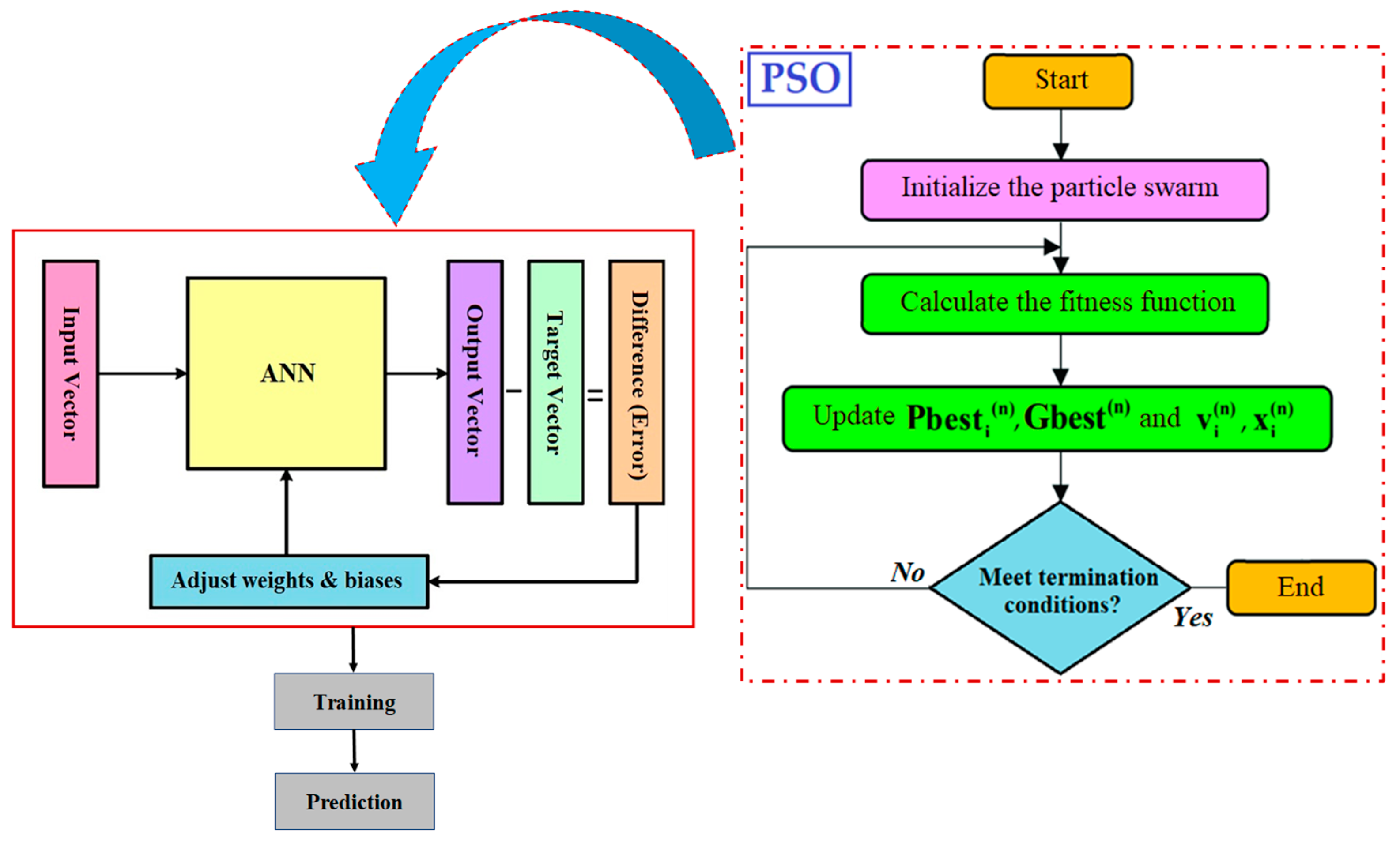
The ANNs are good for learning input-output relationships or patterns. However, they could face local minima and network paralysis problems due to rough weights assigned by learning algorithms such as backpropagation [35]. To overcome these drawbacks, we propose the PSO algorithm to optimize the weights and biases for the ANNs so that the results produced by the ANNs are more accurate as the prediction errors will be minimized. The descriptions of the ANN and PSO algorithms were clearly explained in Section 2.4 and Section 2.5 respectively. To enhance the prediction performance, this study also employed the autocorrelation function (ACF), cross-correlation function (CCF), and data normalization techniques during the data pre-processing phase as described in Section 2.3. For a better understanding, the proposed PSO-ANN approach can also be represented and described by the flowchart in Figure 6:
In Figure 6, the output vector of the ANN network is compared with the target vector, and their difference called “error” is calculated in the form of normalized mean squared error (NMSE); If the average change in the global best (Gbest), corresponding to the NMSE, is greater than the options of the function tolerance (1e-15), the weights and biases of the network will be adjusted or optimized by using the PSO algorithm. The iteration continues until the average change is less than the options of the function tolerance. The proposed PSO-ANN models, for predicting the available energy portion corresponding to the reservoir inflow, can be summarized in the Table 2 below:
Based on the ACF and CCF analyses, the rainfall of the timestep (t) and the inflow of the timestep (t-1) have a good correlation with their own lagged values as well as with the target values i.e., with the converted available energy of the timestep (t) up to three timesteps hence, this study performed the simulation in several scenarios by alternating various input combinations, as summarized in Table 2 for seeking the best prediction model or scenario of the proposed approach to compare with the ANN and NARX approaches as mentioned above whereas the number of output variable for the models was determined to be equal to 1 corresponding to the forecasting objective, and the number of hidden nodes or neurons determined by using the trial-and-error method.

3. Prediction Error

To evaluate the performance of the proposed PSO-ANN prediction models, the three measurement or statistical indicators including root mean square error (RMSE), relative error (RE), and correlation coefficient (r) were calculated and analyzed using Equation (16)–(18) in couple with the Taylor diagrams.
r = i = 1 N ( E m i E ¯ m ) × ( E c i E ¯ c ) [ i = 1 N ( E m i E ¯ m ) 2 × i = 1 N ( E c i E ¯ c ) 2 ]
R M S E = ( i = 1 N ( E m i E c i ) 2 N ) 0.5
R E = | E c i E m i | E c i × 100 %
where E m i represents the target or observed available energy at the time i ; E ¯ m represents the average value of the target or observed available energy at the time i ; E c i represents the predicted available energy at the time i ; E ¯ c i represents the average value of predicted available energy at the time i ; and N represents the number of data points.
The root mean square error (RMSE) and relative error (RE) were used to evaluate the performance of the models whilst the correlation coefficient (r) is used to assess the relations between the target and predicted values as well as to measure the strength in terms of the relationship between the two variables [15].

4. Result and Discussion

A Hybrid model has been developed in this study to predict the available energy portion corresponding to the reservoir incoming flow of Nam Gouang reservoir of the THHP based on the combination of ANN and PSO algorithms described in Section 2.6 together with the ACF, CCF, and data normalization techniques. The historical hydrological and meteorological data of the case study hydropower plant were initially collected ranging from 2013–2023 and then some missing data were filled with the backpropagation technique before preprocessing by proper analysis and normalization. The normalized data was finally partitioned into training and testing clusters at a ratio of approximately 80:20 as described in Section 2.3. In addition to the proposed model, the same datasets were also applied for the ANN and NARX models for comparison purposes.

4.1. Hyperparameter Determination

Input combinations for the feedforward neural network of the proposed approach were determined based on the correlation analysis results in which five scenarios of input combinations were selected and tested as summarized in Table 2. The number of hidden neurons for the neural network was determined by the trial-and-error method and finally selected 30 which is the number that provided the best prediction results. Lastly, the number of output variables was determined to be equal to 1 corresponding to the forecasting objective. With respect to the PSO algorithm, all the hyperparameters were determined by the trial-and-error method and finally obtained the C 1 and C 2 of 1.5 and 2, respectively, ω d a m p (inertia weight damping ratio) of 0.99, and a population (swarm) size of 200.

4.2. Results of the Proposed Approach

Table 3 and Table 4 revealed that the proposed PSO-ANN model of the third scenario (PA3) with the structure (5,30,1) has given the best prediction results with the statistical indicators r = 0.973, RMSE = 22.994 and RE = 1.038 % for the single year of 2022; and r = 0.966, RMSE = 24.846 and RE = 2.853 % for 2023 which were superior over those of the other scenarios i.e., the RMSE and RE of the proposed scenario, both single years, were less than those of other scenarios indicating more accuracy in the forecasting; on the other hand, the correlation coefficient (r) of the proposed scenario was closer to 1 than those of the other scenarios (both years) demonstrating a stronger relationship between predicted and the target values. Hence, the third scenario (PA3) was selected to be the best structure for the proposed approach and for later comparison with the other prediction approaches in this study.

4.3. Training Results

The proposed approach started by adjusting or optimizing the weights and biases of the feedforward neural networks whereas the particle swarm optimization (PSO) algorithm was employed based on the training dataset. The weights and biases were then updated a little bit more with the default function of the network namely, “Trainlm” (a network training function that updates weight and bias values according to Levenberg-Marquardt optimization) during the training process. Several models with different structures have been trained and tested, one best model was then selected based on the results of the statistical indicators, of which the proposed PSO-ANN model of the third scenario (PA3) with the structure (5,30,1) has given the best prediction results.
A cost function applied in the model is the Normalised Mean Square Error (NMSE). The cost function returns an output value, called the “Cost”, which is a numerical value representing the deviation, or degree of error, between the model prediction and the target data; the lower the cost, the lower the deviation (error); hence, the optimal prediction model would have a cost close to 0. Figure 7 depicted the convergence of the best cost in PSO versus the updating iteration for the selected scenario (PA3) in which the best cost value started from 0.61479 in the first iteration and gradually declined to 0.10206 in iteration 842 regarded as the last iteration of the PSO running process.
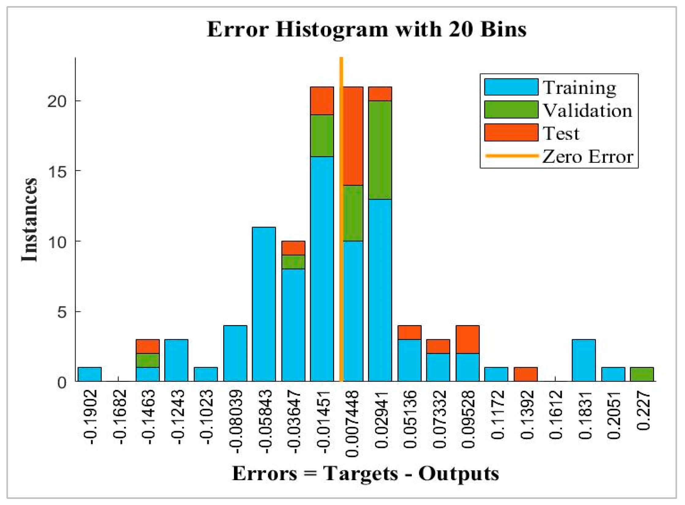
Error histogram represents the histogram of the errors between target values and predicted values after training a feedforward neural network. As these error values indicate how predicted values are different from the target values, hence these can be negative or positive. The graph of the error histogram in Figure 8 visualized errors between the proposed model output and target values during the training process in which the vertical line represents the error at the zero point. In this graph, most of the errors are close to zero points, which demonstrates minor errors in all data clusters, i.e., the training, testing, and validation clusters.
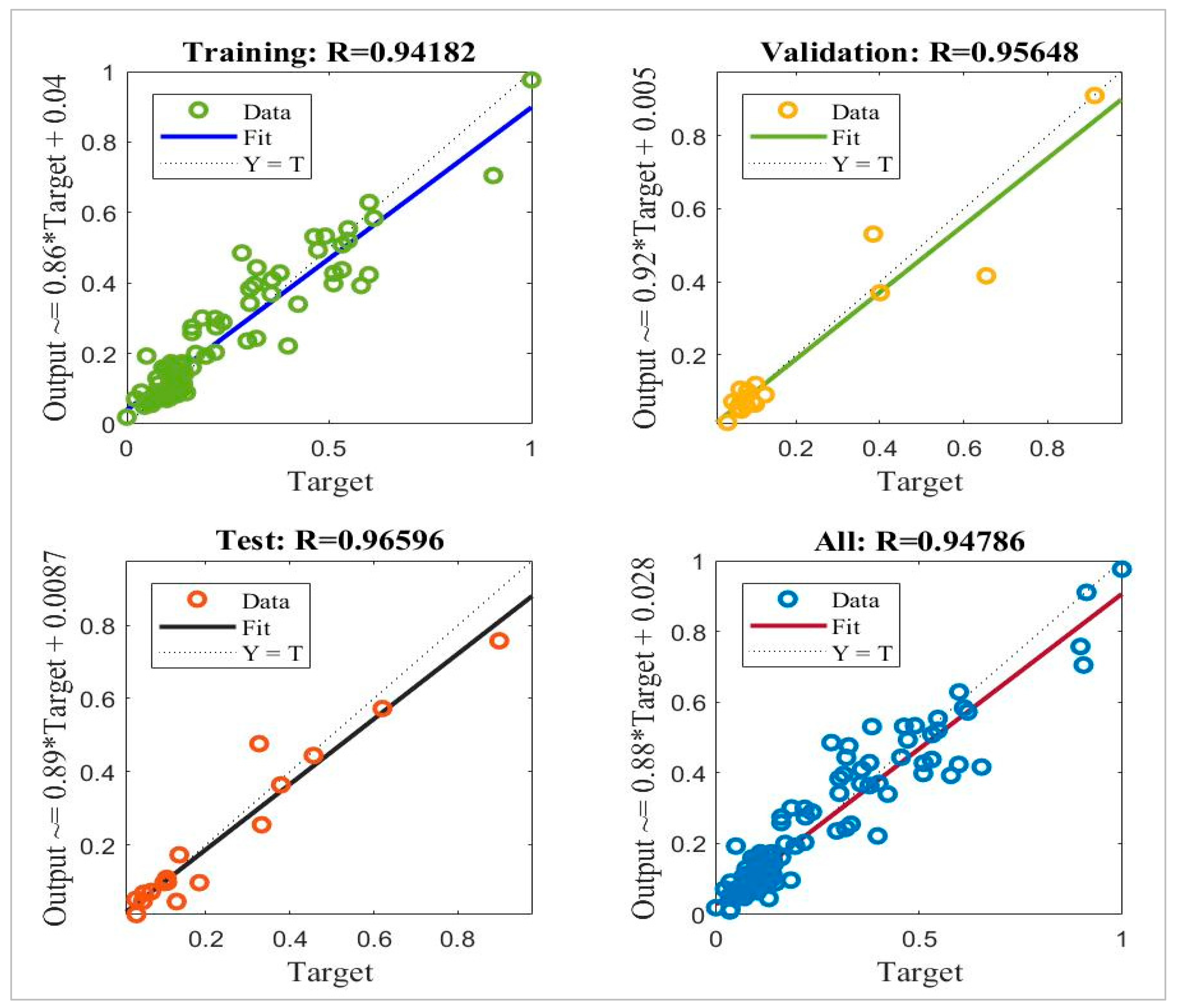
Training regression graphs in Figure 9 representing the correlation between the model output and target values of each data cluster during the process of training (training, validation, testing, and all data clusters) indicated that all the calculated regression coefficients (R) having the directions close to 1 i.e., 0.94182, 0.95648, 0.96596 and 0.94786 for training, validation, test, and all data clusters respectively which mean that the output values of the proposed model (PA3) are having a very good relationship with the target values.
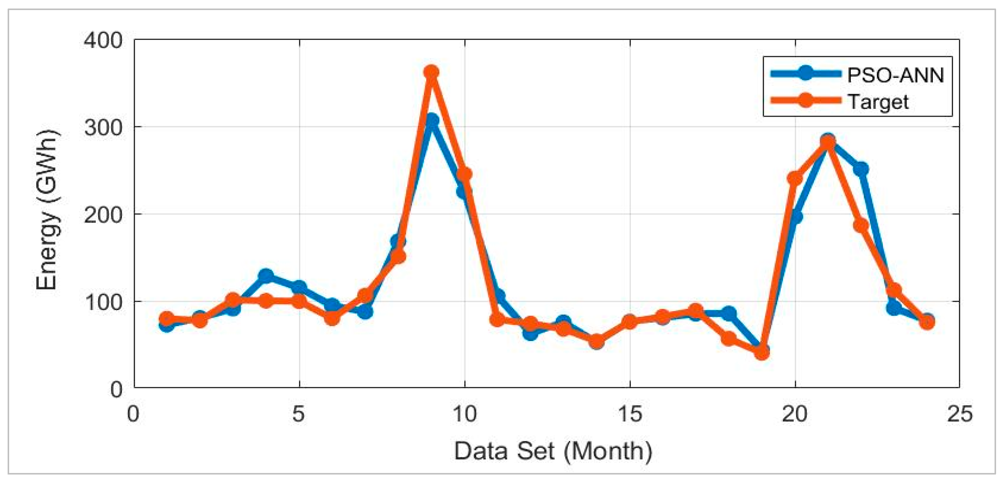
Figure 10 depicts the prediction results of the third scenario (PA3) of the proposed PSO-ANN approach compared to the target values with a total duration of two years i.e., from 2022 to 2023. We observed that the prediction values, represented by the blue curve, agree quite well with the target values, represented by the red curve, all along the testing duration. However, there are still some deviations visualized from the graph both, in the dry period and wet/peak period of the years in which the significant deviation mainly resulted from the high fluctuation and nonstationary of data in the periods of extreme weather conditions.

4.4. Comparison of PSO-ANN, ANN and NARX models

To compare the performance of the proposed PSO-ANN approach of which the third scenario (PA3) has been proved and selected to be the best scenario as described in Section 4.2, the same datasets i.e., the training and testing datasets, comprising of rainfall and lagged inflow, were also applied for the ANN and NARX prediction models and then the best scenario from each approach was selected and compared among the three approaches. In addition to the datasets, the same numbers of input combinations and hidden neurons were also applied for both, ANN and NARX models. The comparison among the best models, of the three approaches, has been made based on the statistical indicators in couple with the Taylor diagrams.
Table 5 and Table 6 revealed that the third scenario of each prediction approach, with the structure (5,30,1) i.e., PA3, A3, and N3 for PSO-ANN, ANN, and NARX models respectively, has given the superior prediction results. We also observed that the third scenario (PA3) of the proposed approach with r = 0.973, RMSE = 22.994 and RE = 1.038 % for the single year of 2022, and r = 0.966, RMSE = 24.846 and RE = 2.853 % for 2023; outperformed those of the ANN and NARX models of which the scenario A3 of the ANN given r = 0.905, RMSE = 36.851 and RE = 7.872 % for the single year of 2022, and r = 0.942, RMSE = 37.238 and RE = 3.619 % for 2023; and the scenario N3 of the NARX given r = 0.939, RMSE = 30.315 and RE = 3.491 % for the single year of 2022, and r = 0.960, RMSE = 28.320 and RE = 3.548 % for 2023 i.e., the root mean square error (RMSE), and relative error (RE) of the proposed PSO-ANN model, both single years, were less than those of the ANN, and NARX models indicating more accuracy in the forecasting; on the other hand, the correlation coefficient (r) of the proposed model was closer to 1 than those of the other models (both years) depicted a stronger correlation between the predicted and target values.
In addition to the clear comparison in Table 5 and Table 6, Figure 11 depicts the predicted values of the three prediction models (scenarios PA3, A3, and N3) versus the target values. We observed that all three prediction curves can track changes of the target (red curve) throughout the testing duration whereas the curve of the proposed PSO-ANN model has a better coincidence than the others, especially during the peak periods of the years indicating superiority in the forecasting. However, the ANN, and NARX models, in some few months during the dry season, performed slightly better than the proposed model, this depicted the advantages and limitations of each approach.
Testing regression graphs with a testing duration of 2 years in Figure 12, illustrate the correlation between each model prediction and target values of which the calculated regression coefficients (R) of the proposed PSO-ANN model at 0.95758 was superior to those of the ANN and NARX models (0.93290, and 0.90303 respectively). In general, Correlation coefficients with a magnitude between 0.9 and 1.0 indicate variables that can be considered very highly correlated. Correlation coefficients with a magnitude between 0.7 and 0.9 indicate variables that can be considered highly correlated. Correlation coefficients with a magnitude between 0.5 and 0.7 indicate variables that can be considered moderately correlated. Whilst the correlation coefficients with a magnitude between 0.3 and 0.5 indicate variables that have a low correlation, and the correlation coefficients with a magnitude less than 0.3 have little if any (linear) correlation.
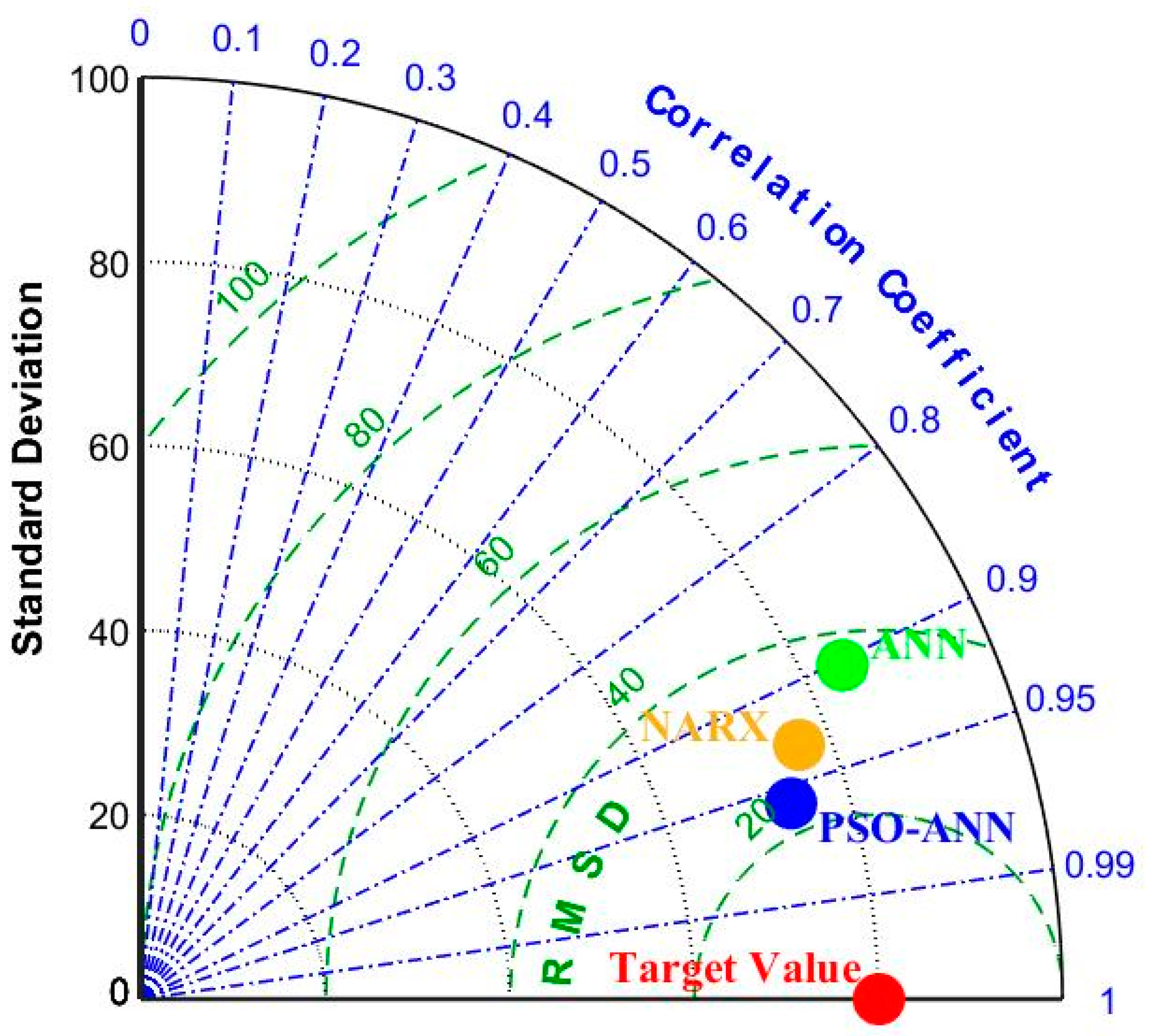
Taylor diagram in Figure 13 illustrates that the root mean square deviation (RMSD), and correlation coefficient (r) of the proposed PSO-ANN model have more vicinity to the target location compared to the ANN and NARX models. With respect to the standard deviation, the ANN and NARX models depicted slightly closer to the target location; however, the standard deviation just indicating how far each value lies from the mean or expected value (A high standard deviation means that values are generally far from the mean, while a low standard deviation indicates that values are clustered close to the means) thus the size of the standard deviation does not reflect a better or worse prediction performance whilst those of the proposed PSO-ANN model herein depicted less than those of the target as well as of the ANN and NARX models. Based on the comparison results illustrated by the Talor diagram in combination with the results of statistical indicators summarized in Table 5 and Table 6, we can conclude that the proposed PSO-ANN approach is more robust and efficient for the available energy prediction for the case study hydropower plant.

5. Conclusion

To forecast the available energy portion that corresponds to the reservoir inflow of the month(s) ahead for ensuring optimal generation planning associated with the revenue maximization as well as the environmental impact prevention, and flood control at the upstream and downstream of the basin, this study has developed the effective hybrid model by integrating Artificial Neural Network (ANN) and Particle Swarm Optimization (PSO) based on hydrological and meteorological data pre-processed by autocorrelation function (AFC), cross-correlation function (CCF), and normalization techniques whereas the Nam Gnouang reservoir of THHP in Laos was selected to be the case study hydropower plant. The model was evaluated using statistical indicators such as correlation coefficient (r), relative error (RE), root mean square error (RMSE), and Taylor diagrams as described in Section 3. Based on the results summarized in Table 5 and Table 6, the third scenario of each prediction approach, with the structure (5,30,1) i.e., PA3, A3, and N3 for PSO-ANN, ANN, and NARX models respectively, has given the best prediction results whereas the proposed PSO-ANN prediction model given r = 0.973, RMSE = 22.994 and RE = 1.038 % for the single year of 2022, and r = 0.966, RMSE = 24.846 and RE = 2.853 % for 2023 demonstrated the superiority over the other models i.e., ANN, and NARX models. Taylor’s diagram in Figure 12 also indicated the same conclusion. These comparison results proved that the proposed approach is more robust and efficient for the available energy forecasting. However, this study has some limitations such as the limited duration of the data, some missing data, limited numbers of hydrological and meteorological factors, and highly fluctuated and nonstationary data significantly affecting the prediction results. For future studies, we suggest considering using the data of longer periods and other relevant hydrological and meteorological variables as well as to seek for an optimal technique for handling climate variability and nonstationary data. In addition, incorporating data from multiple sources by considering using data from satellites, reanalysis products, and ground observations to capture the spatial and temporal variability of climate variables is also recommended.

Author Contributions

Conceptualization, S.K. and V.K.; methodology, S.K. and V.K.; software, S.K. and V.K.; validation, S.K.; formal analysis, S.K.; investigation, S.K.; resources, V.K.; data curation, V.K.; writing—original draft preparation, V.K.; writing—review and editing, S.K.; visualization, S.K.; supervision, S.K.; project administration, S.K.; funding acquisition, S.K. All authors have read and agreed to the published version of the manuscript.

Funding

This research received no external funding.

Data Availability Statement

Not applicable.

Conflicts of Interest

The authors declare no conflicts of interest.

References

  1. Fang, Y.; Ahmadianfar, I.; Samadi-Koucheksaraee, A.; Azarsa, R.; Scholz, M.; Yaseen, Z.M. An accelerated gradient-based optimization development for multi-reservoir hydropower systems optimization. Energy Rep. 2021, 7, 7854–7877. [Google Scholar] [CrossRef]
  2. Long, Y.; Wang, H.; Jiang, C.; Ling, S. Seasonal Inflow Forecasts Using Gridded Precipitation and Soil Moisture Information: Implications for Reservoir Operation. Water Resour. Manag. 2019, 33, 3743–3757. [Google Scholar] [CrossRef]
  3. Li, F.; Ma, G.; Chen, S.; Huang, W. An Ensemble Modeling Approach to Forecast Daily Reservoir Inflow Using Bidirectional Long- and Short-Term Memory (Bi-LSTM), Variational Mode Decomposition (VMD), and Energy Entropy Method. Water Resour. Manag. 2021, 35, 2941–2963. [Google Scholar] [CrossRef]
  4. Rajesh, M.; Anishka, S.; Viksit, P.S.; Arohi, S.; Rehana, S. Improving Short-range Reservoir Inflow Forecasts with Machine Learning Model Combination. Water Resour. Manag. 2022, 37, 75–90. [Google Scholar] [CrossRef]
  5. Yu, J.; Chang, W.-S.; Dong, Y. Building Energy Prediction Models and Related Uncertainties: A Review. Buildings 2022, 12, 1284. [Google Scholar] [CrossRef]
  6. Khorram, S.; Jehbez, N. A Hybrid CNN-LSTM Approach for Monthly Reservoir Inflow Forecasting. Water Resour. Manag. 2023, 37, 4097–4121. [Google Scholar] [CrossRef]
  7. Saab, S.M.; Othman, F.; Tan, C.G.; Allawi, M.F.; Sherif, M.; El-Shafie, A. Utilizing deep learning machine for inflow forecasting in two different environment regions: a case study of a tropical and semi-arid region. Appl. Water Sci. 2022, 12, 272. [Google Scholar] [CrossRef]
  8. Latif, S.D.; Ahmed, A.N. A review of deep learning and machine learning techniques for hydrological inflow forecasting. Environ. Dev. Sustain. 2023, 25, 12189–12216. [Google Scholar] [CrossRef]
  9. Awan, J.A.; Bae, D.-H. Improving ANFIS Based Model for Long-term Dam Inflow Prediction by Incorporating Monthly Rainfall Forecasts. Water Resour. Manag. 2014, 28, 1185–1199. [Google Scholar] [CrossRef]
  10. Chang, F. J. , Lo, Y. C., Chen, P. A., Chang, L. C., & Shieh, M. C. Multi-step-ahead reservoir inflow forecasting by artificial intelligence techniques. Smart Innovation System and Technology 2015, 30, 235–249. [Google Scholar] [CrossRef]
  11. Chiamsathit, C.; Adeloye, A.J.; Bankaru-Swamy, S. Inflow forecasting using Artificial Neural Networks for reservoir operation. Proc. Int. Assoc. Hydrol. Sci. 2019, 373, 209–214. [Google Scholar] [CrossRef]
  12. Babaei, M.; Moeini, R.; Ehsanzadeh, E. Artificial Neural Network and Support Vector Machine Models for Inflow Prediction of Dam Reservoir (Case Study: Zayandehroud Dam Reservoir). Water Resour. Manag. 2019, 33, 2203–2218. [Google Scholar] [CrossRef]
  13. Noorbeh, P.; Noorbeh, P.; Roozbahani, A.; Roozbahani, A.; Moghaddam, H.K.; Moghaddam, H.K. Annual and Monthly Dam Inflow Prediction Using Bayesian Networks. Water Resour. Manag. 2020, 34, 2933–2951. [Google Scholar] [CrossRef]
  14. Hadiyan, P.P.; Moeini, R.; Ehsanzadeh, E.; Karvanpour, M. Trend Analysis of Water Inflow Into the Dam Reservoirs Under Future Conditions Predicted By Dynamic NAR and NARX Models. Water Resour. Manag. 2022, 36, 2703–2723. [Google Scholar] [CrossRef]
  15. Hanoon, M.S.; Ahmed, A.N.; Razzaq, A.; Oudah, A.Y.; Alkhayyat, A.; Huang, Y.F.; Kumar, P.; El-Shafie, A. Prediction of hydropower generation via machine learning algorithms at three Gorges Dam, China. Ain Shams Eng. J. 2023, 14. [Google Scholar] [CrossRef]
  16. Fallah, S.N.; Deo, R.C.; Shojafar, M.; Conti, M.; Shamshirband, S. Computational intelligence approaches for energy load forecasting in smart energy management grids: State of the art, future challenges, and research directions. Smart Grid 2018, 11, 596. [Google Scholar] [CrossRef]
  17. Moeeni, H.; Bonakdari, H.; Ebtehaj, I. Monthly reservoir inflow forecasting using a new hybrid SARIMA genetic programming approach. J. Earth Syst. Sci. 2017, 126, 18. [Google Scholar] [CrossRef]
  18. Qi, Y.; Zhou, Z.; Yang, L.; Quan, Y.; Miao, Q. A Decomposition-Ensemble Learning Model Based on LSTM Neural Network for Daily Reservoir Inflow Forecasting. Water Resour. Manag. 2019, 33, 4123–4139. [Google Scholar] [CrossRef]
  19. Feizi, H.; Apaydin, H.; Sattari, M.T.; Colak, M.S.; Sibtain, M. Improving reservoir inflow prediction via rolling window and deep learning-based multi-model approach: case study from Ermenek Dam, Turkey. Stoch. Environ. Res. Risk Assess. 2022, 36, 3149–3169. [Google Scholar] [CrossRef]
  20. Ghazali, M.; Honar, T.; Nikoo, M.R. A fusion-based neural network methodology for monthly reservoir inflow prediction using MODIS products. Hydrol. Sci. J. 2019, 63, 2076–2096. [Google Scholar] [CrossRef]
  21. Bayat, N.; Park, J.-H. Particle Swarm Optimization Based Demand Response Using Artificial Neural Network Based Load Prediction. 2023 North American Power Symposium (NAPS).
  22. Panyadee, P.; Champrasert, P.; Aryupong, C. Water level prediction using artificial neural network with particle swarm optimization model. Natural Disaster Management 2017. [Google Scholar] [CrossRef]
  23. Rosli, N.S.; Ibrahim, R.; Ismail, I. Neural network model with particle swarm optimization for prediction in gas metering systems. Intelligent and Advanced System 2017. [Google Scholar] [CrossRef]
  24. Hamada, M.; Hassan, M. Artificial Neural Networks and Particle Swarm Optimization Algorithms for Preference Prediction in Multi-Criteria Recommender Systems. Informatics 2018, 5, 25. [Google Scholar] [CrossRef]
  25. Fadlallah, S.O.; Anderson, T.N.; Nates, R.J. Artificial Neural Network–Particle Swarm Optimization (ANN-PSO) Approach for Behaviour Prediction and Structural Optimization of Lightweight Sandwich Composite Heliostats. Arab. J. Sci. Eng. 2021, 46, 12721–12742. [Google Scholar] [CrossRef]
  26. Seguini, M.; Boutchicha, D.; Nedjar, D. Crack prediction in pipeline using ANN-PSO based on numerical and experimental modal analysis. Smart Structures and System 2021, 27, 507–523. [Google Scholar] [CrossRef]
  27. Lu, H.; Wu, J.; Ruan, Y.; Qian, F.; Meng, H.; Gao, Y.; Xu, T. A multi-source transfer learning model based on LSTM and domain adaptation for building energy prediction. Int. J. Electr. Power Energy Syst. 2023, 149, 109024. [Google Scholar] [CrossRef]
  28. Moayed, F.A.; Shell, R.L. Application of Artificial Neural Network Models in Occupational Safety and Health Utilizing Ordinal Variables. Ann. Work. Expo. Heal. 2021, 55, 132–142. [Google Scholar] [CrossRef]
  29. Tzeng, F.-Y.; Ma, K.-L. Opening the black box | data driven visualization of neural networks. Computer Science 2005. [Google Scholar] [CrossRef]
  30. Bhadeshia, H.K.D.H. Neural Networks in Materials Science. ISIJ Int. 1999, 39, 966–979. [Google Scholar] [CrossRef]
  31. Shami, T.M.; El-Saleh, A.A.; Alswaitti, M.; Al-Tashi, Q.; Summakieh, M.A.; Mirjalili, S. Particle Swarm Optimization: A Comprehensive Survey. IEEE Access 2022, 10, 10031–10061. [Google Scholar] [CrossRef]
  32. Wang, R.; Hao, K.; Chen, L.; Wang, T.; Jiang, C. A novel hybrid particle swarm optimization using adaptive strategy. Inf. Sci. 2021, 579, 231–250. [Google Scholar] [CrossRef]
  33. Semero, Y.K.; Zheng, D.; Zhang, J. A PSO-ANFIS based Hybrid Approach for Short Term PV Power Prediction in Microgrids. Electr. Power Components Syst. 2018, 46, 95–103. [Google Scholar] [CrossRef]
  34. Kennedy, J. The behavior of particles. In Proceedings of the Transactions on Petri Nets and Other Models of Concurrency XV; Springer: Berlin/Heidelberg, Germany, 1998; pp. 579–589. [Google Scholar]
  35. Sharma, D.K.; Hota, H.S.; Brown, K.; Handa, R. Integration of genetic algorithm with artificial neural network for stock market forecasting. Int. J. Syst. Assur. Eng. Manag. 2021, 13, 828–841. [Google Scholar] [CrossRef]
Disclaimer/Publisher’s Note: The statements, opinions, and data contained in all publications are solely those of the individual author(s) and contributor(s) and not of MDPI and/or the editor(s). MDPI and/or the editor(s) disclaim responsibility for any injury to people or property resulting from any ideas, methods, instructions, or products referred to in the content.
Figure 1. Research methodology flowchart.
Preprints 112801 g001
Figure 2. Map of Nam Gnouang reservoir of THHP.
Preprints 112801 g002
Figure 3. Hydropower plant energy schematic overview.
Preprints 112801 g003
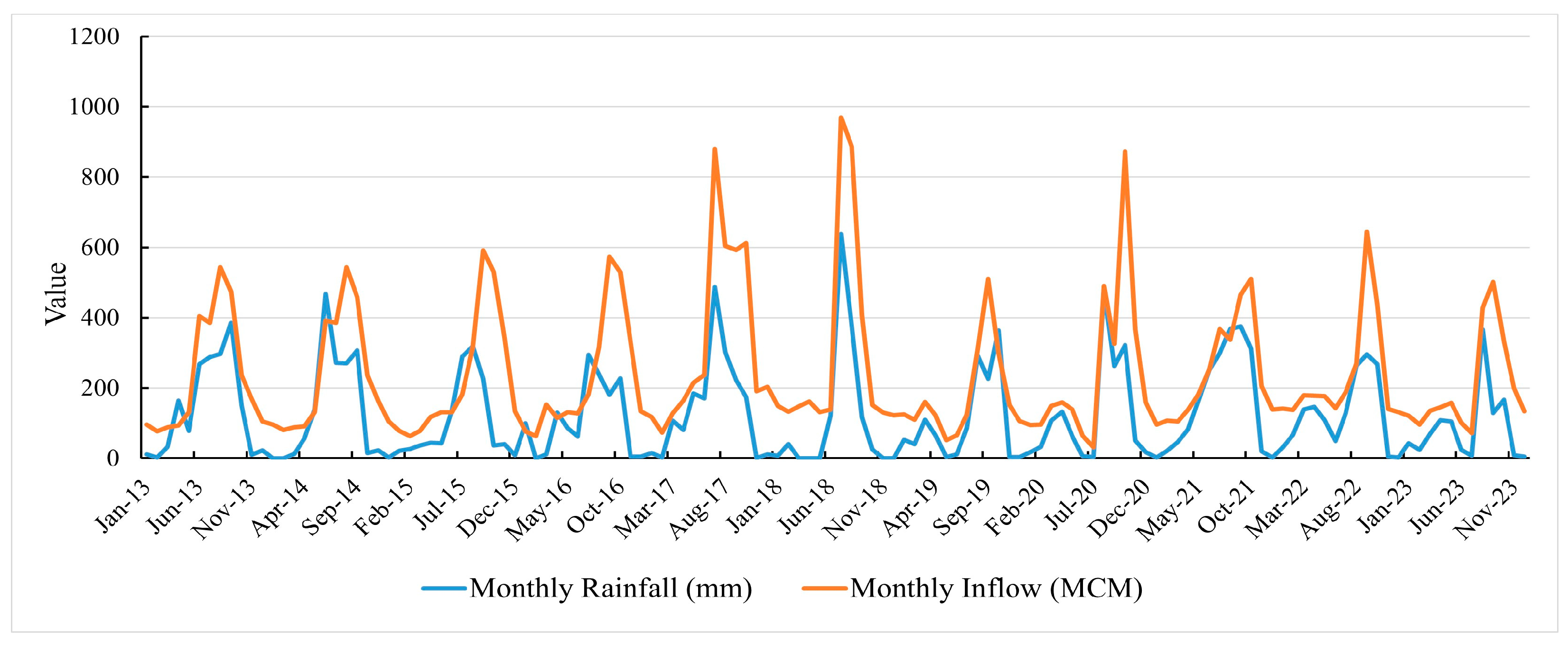
Figure 4. Original data of Nam Gnouang reservoir.
Preprints 112801 g004
Figure 5. Feedforward Neural Network.
Preprints 112801 g005
Figure 6. PSO-ANN approach.
Preprints 112801 g006
Figure 7. Best cost of the selected scenario (PA3).
Preprints 112801 g007
Figure 8. Training error histogram (PA3).
Preprints 112801 g008
Figure 9. Training regression (PA3).
Preprints 112801 g009
Figure 10. PSO-ANN prediction vs. target values (PA3).
Preprints 112801 g010
Figure 11. Comparison among the three models with the target values.
Preprints 112801 g011
Figure 12. Regression comparison among the three models (testing duration of 2 years).
Preprints 112801 g012
Figure 13. Taylor diagram of the three models vs. the target.
Preprints 112801 g013
Table 1. Basic design specifications of the case study hydropower plant.
Design Feature Specification
Original Weir Dam (run-of-river type):
Concrete Gravity Free Overflow Weir:
Spillway radial gates
Head Pond Full Supply Level
Two concrete-lined headrace tunnels length
Installed capacity

NG Dam (storage type):
Concrete Gravity Dam
Reservoir Full Supply Level
Max Actual Storage Volume
Spillway radial gates
Installed capacity
268 x 27 m (L x H)
2
400 m asl
5,289 m and 5,496 m
2 x 110 MW (+ 220 MW)


480 x 65 m (L x H)
455 m asl
2,430 MCM
5
2 x 30 MW
Table 2. Summary of the various combination input designs.
Model Scenario Input combinations Output
SC1 R(t), I(t-1)
SC2
SC3
SC4
SC5
R(t), R(t-1), I(t-1), I(t-2)
R(t), R(t-1), I(t-1), I(t-2),I(t-3)
R(t), R(t-1), R(t-2), I(t-1), I(t-2)
R(t), R(t-1), R(t-2), I(t-1), I(t-2),I(t-3)
E(t)
* Notes: R(t) = Rainfall of month (t) [mm]. R(t-1) = Rainfall of month (t-1) [mm]. R(t-2) = Rainfall of month (t-2) [mm]. I(t-1) = Inflow of month (t-1) [hm3]. I(t-2) = Inflow of month (t-2) [hm3]. I(t-3) = Inflow of month (t-3) [hm3]. E(t) = Energy of month (t) [GWh].
Table 3. Results by statistical indicators of the PSO-ANN models 2022.
Model Scenarios Model Input
combinations
Model Output Different
Models
Model Structures r RMSE RE
PA1
PA2
PA3
PA4
PA5
R(t), I(t-1)
R(t), R(t-1), I(t-1), I(t-2)
R(t), R(t-1), I(t-1), I(t-2),I(t-3)
R(t), R(t-1), R(t-2), I(t-1), I(t-2)
R(t), R(t-1), R(t-2), I(t-1), I(t-2),I(t-3)
E(t)
E(t)
E(t)
E(t)
E(t)
PSO-ANN
PSO-ANN
PSO-ANN
PSO-ANN
PSO-ANN
(2,30,1)
(4,30,1)
(5,30,1)
(5,30,1)
(6,30,1)
0.951
0.968
0.973
0.942
0.930
38.168
33.261
22.994
32.924
34.354
8.261
18.459
1.038
7.847
3.662
Table 4. Results by statistical indicators of the PSO-ANN models 2023.
Model Scenarios Model Input
combinations
Model Output Different
Models
Model Structures r RMSE RE
PA1
PA2
PA3
PA4
PA5
R(t), I(t-1)
R(t), R(t-1), I(t-1), I(t-2)
R(t), R(t-1), I(t-1), I(t-2),I(t-3)
R(t), R(t-1), R(t-2), I(t-1), I(t-2)
R(t), R(t-1), R(t-2), I(t-1), I(t-2),I(t-3)
E(t)
E(t)
E(t)
E(t)
E(t)
PSO-ANN
PSO-ANN
PSO-ANN
PSO-ANN
PSO-ANN
(2,30,1)
(4,30,1)
(5,30,1)
(5,30,1)
(6,30,1)
0.905
0.965
0.966
0.930
0.956
44.925
30.668
24.846
36.757
27.934
15.059
5.832
2.853
7.928
3.001
Table 5. Results by statistical indicators of all models 2022.
Model Scenarios Model Input
combinations
Model Output Different
Models
Model Structures r RMSE RE
PA1
PA2
PA3
PA4
PA5

A1
A2
A3
A4
A5

N1
N2
N3
N4
N5
R(t), I(t-1)
R(t), R(t-1), I(t-1), I(t-2)
R(t), R(t-1), I(t-1), I(t-2),I(t-3)
R(t), R(t-1), R(t-2), I(t-1), I(t-2)
R(t), R(t-1), R(t-2), I(t-1), I(t-2),I(t-3)

R(t), I(t-1)
R(t), R(t-1), I(t-1), I(t-2)
R(t), R(t-1), I(t-1), I(t-2),I(t-3)
R(t), R(t-1), R(t-2), I(t-1), I(t-2)
R(t), R(t-1), R(t-2), I(t-1), I(t-2),I(t-3)

R(t), I(t-1)
R(t), R(t-1), I(t-1), I(t-2)
R(t), R(t-1), I(t-1), I(t-2),I(t-3)
R(t), R(t-1), R(t-2), I(t-1), I(t-2)
R(t), R(t-1), R(t-2), I(t-1), I(t-2),I(t-3)
E(t)
E(t)
E(t)
E(t)
E(t)

E(t)
E(t)
E(t)
E(t)
E(t)

E(t)
E(t)
E(t)
E(t)
E(t)
PSO-ANN
PSO-ANN
PSO-ANN
PSO-ANN
PSO-ANN

ANN
ANN
ANN
ANN
ANN

NARX
NARX
NARX
NARX
NARX
(2,30,1)
(4,30,1)
(5,30,1)
(5,30,1)
(6,30,1)

(2,30,1)
(4,30,1)
(5,30,1)
(5,30,1)
(6,30,1)

(2,30,1)
(4,30,1)
(5,30,1)
(5,30,1)
(6,30,1)
0.951
0.968
0.973
0.942
0.930

0.894
0.900
0.905
0.821
0.775

0.894
0.832
0.939
0.796
0.844
38.168
33.261
22.994
32.924
34.354

43.444
55.512
36.851
76.032
55.106

40.182
55.317
30.315
51.605
45.577
8.261
18.459
1.038
7.847
3.662

18.178
41.521
7.872
27.723
10.051

3.030
16.462
3.491
7.338
4.250
Table 6. Results by statistical indicators of all models 2023.
Model Scenarios Model Input
combinations
Model Output Different
Models
Model Structures r RMSE RE
PA1
PA2
PA3
PA4
PA5

A1
A2
A3
A4
A5

N1
N2
N3
N4
N5
R(t), I(t-1)
R(t), R(t-1), I(t-1), I(t-2)
R(t), R(t-1), I(t-1), I(t-2),I(t-3)
R(t), R(t-1), R(t-2), I(t-1), I(t-2)
R(t), R(t-1), R(t-2), I(t-1), I(t-2),I(t-3)

R(t), I(t-1)
R(t), R(t-1), I(t-1), I(t-2)
R(t), R(t-1), I(t-1), I(t-2),I(t-3)
R(t), R(t-1), R(t-2), I(t-1), I(t-2)
R(t), R(t-1), R(t-2), I(t-1), I(t-2),I(t-3)

R(t), I(t-1)
R(t), R(t-1), I(t-1), I(t-2)
R(t), R(t-1), I(t-1), I(t-2),I(t-3)
R(t), R(t-1), R(t-2), I(t-1), I(t-2)
R(t), R(t-1), R(t-2), I(t-1), I(t-2),I(t-3)
E(t)
E(t)
E(t)
E(t)
E(t)

E(t)
E(t)
E(t)
E(t)
E(t)

E(t)
E(t)
E(t)
E(t)
E(t)
PSO-ANN
PSO-ANN
PSO-ANN
PSO-ANN
PSO-ANN

ANN
ANN
ANN
ANN
ANN

NARX
NARX
NARX
NARX
NARX
(2,30,1)
(4,30,1)
(5,30,1)
(5,30,1)
(6,30,1)

(2,30,1)
(4,30,1)
(5,30,1)
(5,30,1)
(6,30,1)

(2,30,1)
(4,30,1)
(5,30,1)
(5,30,1)
(6,30,1)
0.905
0.965
0.966
0.930
0.956

0.909
0.873
0.942
0.910
0.821

0.905
0.922
0.960
0.943
0.911
44.925
30.668
24.846
36.757
27.934

44.268
51.048
37.238
55.710
57.602

43.566
39.719
28.320
34.179
39.604
15.059
5.832
2.853
7.928
3.001

24.058
28.574
3.619
25.550
11.466

14.521
5.724
3.548
6.101
7.106
Disclaimer/Publisher’s Note: The statements, opinions and data contained in all publications are solely those of the individual author(s) and contributor(s) and not of MDPI and/or the editor(s). MDPI and/or the editor(s) disclaim responsibility for any injury to people or property resulting from any ideas, methods, instructions or products referred to in the content.
Copyright: This open access article is published under a Creative Commons CC BY 4.0 license, which permit the free download, distribution, and reuse, provided that the author and preprint are cited in any reuse.
Prerpints.org logo

Preprints.org is a free preprint server supported by MDPI in Basel, Switzerland.

Subscribe

© 2024 MDPI (Basel, Switzerland) unless otherwise stated