Representation Learning-Based Graph and Generative Network for Hyperspectral Small Target Detection

Preprint

Article

Representation Learning-Based Graph and Generative Network for Hyperspectral Small Target Detection

Altmetrics

Downloads

108

Views

Comments

A peer-reviewed article of this preprint also exists.

This version is not peer-reviewed

Submitted:

26 July 2024

Posted:

27 July 2024

You are already at the latest version

Alerts

Abstract

Hyperspectral small target detection (HSTD) is a promising pixel-level detection task. However, due to the low contrast and imbalance number between the target and background spatially and high dimensions spectrally, it is a challenging one. To address these issues, this work proposes a representation learning-based graph and generative network for hyperspectral small target detection. The model builds a fusion network through frequency representation for HSTD, where the novel architecture incorporates irregular topological data and the spatial-spectral feature to improve its representation ability. Firstly, a graph convolutional network (GCN) module better models the non-local topological relationship between samples to represent the hyperspectral scene’s underlying data structure. The mini-batch-training pattern of the GCN decreases the high computational cost of building an adjacency matrix for high-dimensional data sets. In parallel, the generative model enhances the differentiation reconstruction and the deep feature representation ability with respect to the target spectral signature. Finally, a fusion module compensates for the extracted different types of HS features and integrates their complementary merits for hyperspectral data interpretation while increasing detection and background suppression capabilities. Experiments on different hyperspectral data sets demonstrate the advantages of the proposed architecture.

Keywords:

Subject: Computer Science and Mathematics - Artificial Intelligence and Machine Learning

1. Introduction

Hyperspectral images (HSIs) are widely applied in land cover mapping, agriculture, urban planning, and other applications [1]. The high spectral resolution of HSIs enables the detection of a wide range of small and specific targets through spatial analysis or visual inspection[2]. In HSIs, the definition of small targets typically depends on the specific application scenario and task requirements. For instance, if the task is to detect traffic signs in HSIs, small targets may be defined as objects with traffic sign characteristics, with their size determined by the actual dimensions of traffic signs. These small targets usually have dimensions ranging from the pixel level to a few dozen pixels. Although their size may be minuscule compared to the entire image, they hold significant importance in specific contexts. Additionally, the semantic content of small targets may carry particular significance; for example, HSIs may include various objects such as vehicles, buildings, and people.

In this topical area, the most challenging targets in HSIs have the following characteristics: 1) Weak contrast: HSIs with their high spectral resolution but lower spatial resolution depict spatially and spectrally complex scenes, affected by sensor noise and material mixing; the targets are immersed in this context, leading to usually weak contrast and low signal-to-noise ratio (SNR) values. 2) Limited numbers: Due to the coarse spatial resolution, a target often occupies only one or a few pixels in a scene, which provides limited training samples. 3) Spectral complexity: HSI contains abundant spectral information. This leads to a very large dimension of the feature space, to strong data correlation in different bands, extensive data redundancy, and eventually long computational times. In HSTD, the background typically refers to the parts of the image that do not contain the target. Compared to the target, the background usually has a higher similarity in color, texture, or spectral characteristics with the surrounding area, resulting in lower contrast within the image. This means it does not display distinct characteristics or significant differences from the surrounding regions. Background areas generally exhibit a certain level of consistency, with neighboring pixels having high similarity in their attributes. For example, a green grass field, a blue sky, or a gray building wall. This consistency means that the background may show relatively uniform spectral characteristics. Additionally, the background usually occupies a larger portion of the image and may have characteristics related to the environment, such as terrain, vegetation types, and building structures. These characteristics help distinguish the background from the target area. Accurately defining and modeling the background is crucial for improving the accuracy and robustness of target detection.

Based on these characteristics, the algorithms for HSI target extraction may be roughly subdivided into two big families: more traditional signal detection methods and more recent data-driven pattern recognition and machine learning methods.

Traditionally, detection involves transforming the spectral characteristics of target and background pixels into a specific feature space based on predefined criteria [4]. Targets and backgrounds occupy distinct positions within this space, allowing targets to be extracted using threshold or clustering techniques. In this research domain, diverse descriptions of background models have led to the development of various mathematical models [5,6,7,8] for characterizing spectral pixel changes.

A first category of algorithms in this family are the spectral information-based models, when the target and background spectral signatures are supposed to be generated by a linear combination of end member spectra. The Orthogonal Subspace Projection (OSP) [9] and the Adaptive Subspace Detector (ASD) [10] are two representative subspace-based target detection algorithms. OSP employs a signal detection method to remove background features by projecting each pixel’s spectral vector onto a subspace. However, the fact that the same object may have distinct spectra, and the same spectra may appear in different objects because of spectral variation caused by the atmosphere, by sensor noise, and the mixing of multiple spectra makes the identification of a target more challenging in reality due to imaging technology limitations [11]. To tackle this issue, Chen et al. proposed an adaptive target pixel selection approach based on spectral similarity and spatial relationship characteristics [12], which addresses the pixel selection problem.

A second category is statistical methods. These approaches presume a background that follows a specified distribution and then establish whether or not the target exists by looking for outliers with respect to this distribution. The adaptive cosine consistency estimator (ACE) [13] and the adaptive matched filter (AMF) [14], are among the techniques in this group, and are both based on the generalized likelihood ratio-based detection test (GLRT) method [15].

Both ACE and AMF are spectral detectors that measure the distance between target features and data samples. ACE can be considered as a special case of a spectral angle-based detector. AMF was designed according to the hypothesis testing method of Gaussian distribution. The third category is the representation-based methods without assumption of data distribution, e.g., constrained energy minimization (CEM) [16,17], hierarchical CEM (hCEM) [18], ensemble-based CEM (eCEM) [19], sCEM [20], target-constrained inference-minimized filter (TCIMF), and sparse representation (ST)-based methods [21]. Among these approaches, the classic and foundational CEM method constrains targets and minimizes data sample variance, and the TCIMF method combines CEM and OSP.

The most recent deep learning methods for target detection are mainly based on data representations involving kernels, sparse representations, manifold learning, and unsupervised learning. Specifically, methods based on sparse representation take into account the connections between samples in the sparse representation space. The Combined Sparse and Collaborative Representation (CSCR) [22] and the Dual Sparsity Constrained (DSC) [23] methods are examples of sparse representation. However, the requirement for exact pixel-wise labeling makes the task of achieving good performance an expensive one. To address the challenge of obtaining pixel-level accurate labels, Jiao et al. proposed a semantic multiple-instance neural network with contrastive and sparse attention fusion [24]. Kernel-based transformations [25] are employed to address the linear inseparability issue between targets and background in the original feature space. Gaussian radial basic kernel functions are commonly used, but there is still a lack of rules for choosing the best performing kernel. Besides, in [26], manifold learning is employed to learn a subspace that encodes discriminative information. Finally, for unsupervised learning methods, an effective feature extraction method based on unsupervised networks is proposed to mine intrinsic properties underlying HSIs. The spectral regularization is imposed on autoencoder (AE) and variational AE (VAE) to emphasize spectral consistency [27]. Another novel network block with the region-of-interest feature transformation and the multi-scale spectral-attention module is also proposed to reduce the spatial and spectral redundancies simultaneously and provide strong discrimination [28].

While recent advancements have shown increased effectiveness, challenges remain in efficiently tuning a large number of hyperparameters and in obtaining accurate labels [29,30]. Moreover, the statistical features extracted by GAN-based methods often overlook the potential topological structure information. Such phenomenon greatly limits the ability to capture non-local topological relationships to better represent the underlying data structure of HSI. Thus, the representative of features are not fully exploited and utilized to preserve the most valuable information through different networks. Detecting the location and shape of small targets with weak contrast against the background remains a significant challenge. Therefore, this paper proposes a deep representative model of the graph and generative learning fusion network with frequency representation. The goal is to learn a stable and robust model based on an effective feature representation. The primary contributions of this study are summarized as follows:

We explore a collaboration framework for HSTD with less computation cost and high accuracy. Under the framework, the feature extraction from the graph and generative learning compensates each other. As far as we are concerned, it is the first work to explore the collaborative relationship between the graph and generative learning in HSTD.
The graph learning module is established for HSTD. The GCN module aims at compensating for the information loss of details caused by the encoder and decoder via aggregating features from multiple adjacent levels. As a result, the detailed features of small targets can be propagated to the deeper layers of the network.
The primary mini batch GCN branch for HSTD is designed by following an explicit design principle derived from the graph method to solve high computational costs. It enables the graph to enhance the feature and suppress noise, effectively dealing with background interference and retaining the target details.
A spectral-constrained filter is used to retain the different frequency components. Frequency learning is introduced into data preparation in coarse candidate sample selection, favoring strong relevance among pixels of the same object.

The remainder of this article is structured as follows. Section 2 provides a brief overview of graph learning. Section 3 elaborates on the proposed GCN and introduces the fusion module. Extensive experiments and analyses are given in Section 4. Section 5 provides some conclusions.

2. Graph Learning

A graph describes the one-to-many relations in a non-Euclidean space [31], including directed and un-directed patterns. It can be mixed with a neural network to design Graph Convolution Networks (GCNs), Graph Attention Networks (GATs), Graph Autoencoders (GAEs), Graph Generative Networks (GGNs), and Graph Spatial-Temporal Networks (GSTNs) [32].

Among the graph-based networks mentioned above, this work focuses on GCNs, a set of neural networks that infers convolution from traditional data to graph data. Specifically, the convolution operation can be applied within a graph structure, where the key operation involves learning a mapping function. In this work, an undirected graph models the relationship between the spectral features and performs feature extraction [33]. In matrix form, the layer-wise propagation rule of the multi-layer GCN is defined as:

H^{(k)} = σ (D^{- \frac{1}{2}} \tilde{A} D^{- \frac{1}{2}} H^{(k - 1)} W^{(k)})

(1)

where

H^{(k)}

denotes the output in the

(k)

-th layer.

σ (\cdot)

is the activation function with respect to the weights to-be-learned and the biases of all layers. D represents a diagonal matrix of node degrees.

\tilde{A} = A + I

represents the adjacency matrix

A

of undirected graph G added with the identity matrix

I

of proper size throughout this article.

Deep learning-based approaches for HSIs based on Graph Learning are increasingly widely used, especially for detection and classification. For instance, weighted feature fusion of convolutional neural network (CNN) and graph attention network (WFCG) exploits the complementing characteristics of superpixel-based GAT and pixel-based CNN [34,35]. Finally, a robust self-ensembling network (RSEN) is proposed, comprising a base and ensemble network, which achieves satisfactory results even with limited sample sizes [36].

3. Proposed Methodology

3.1. Overall Framework

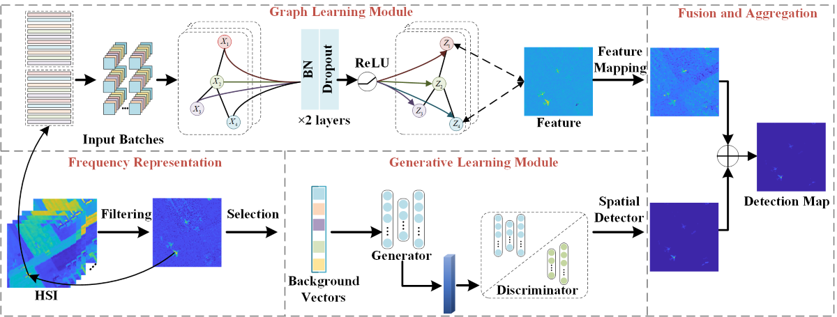
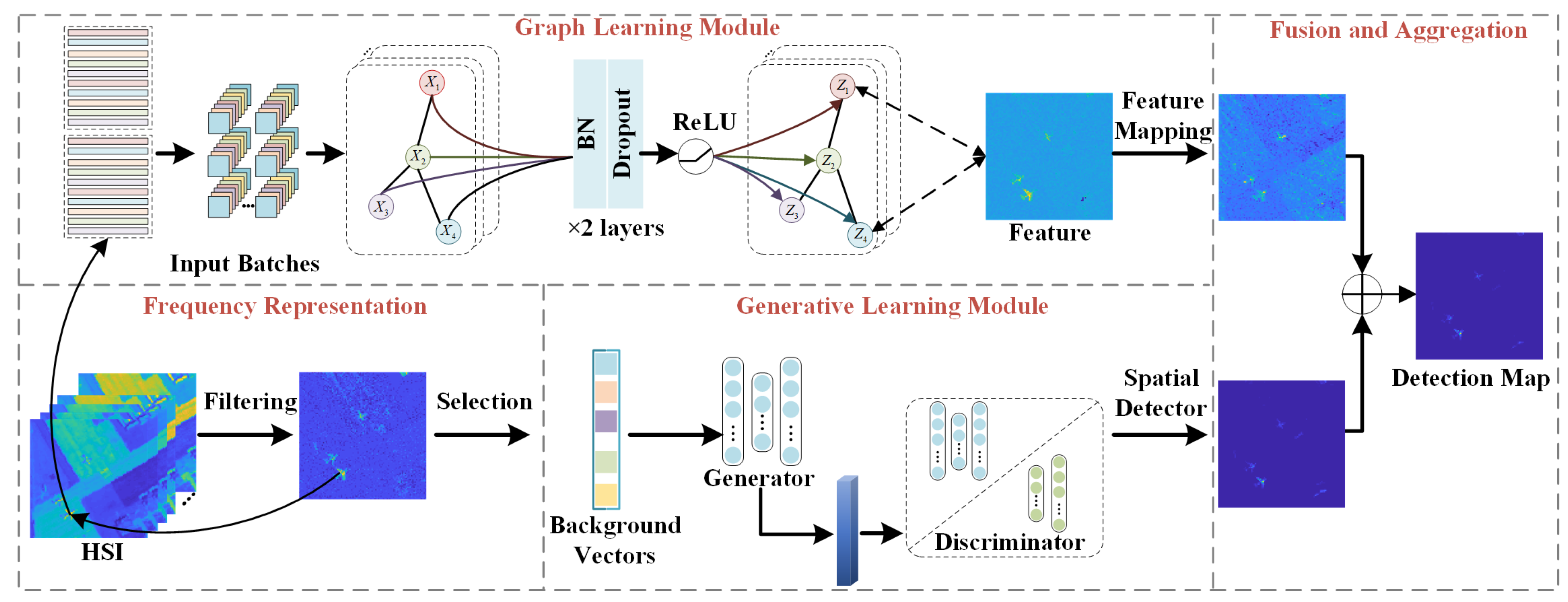
This section proposes a fusion graph and generative learning network with frequency representation. The architecture of this method is shown in Figure 1, which consists of the GCN and GAN modules, to represent different types of features, with help from the frequency learning to select the initial pseudo labels. The graph learning module’s graph structure defines topological interactions in small batches to minimize computer resource requirements and refine the spatial features from HSI. The idea is to obtain spatially and spectrally representative information from the latent and reconstructed domains. The information is based on components extracted in the generative learning module to leverage the discriminative capacity of GAN models. A fusion module then exploits the association between these two complementary modules.

The description of problem formulation is as follows. Let’s denote the HSI by

X \in R^{M \times N \times C}

, where M, N, C are the three dimensions of the image. The input HSI can is the collection of background set

X_{B}

and target set

X_{T}

, i.e.

X = [X_{B}, X_{T}]

, and

X_{B} \cup X_{T} = X

X_{B} \cap X_{T} = ϕ

. According to these definitions, the establishment of the overall model is

(X_{g_{1}}, X_{g_{2}}) = ψ (X, d; X = X_{B} \cup X_{T})

(2)

where

X_{g_{1}} = f_{g r a p h} (X_{i n}, L, w, b)

is the output of the GCN function

f_{g r a p h} (\cdot)

L

is the Laplacian matrix.

X_{g_{2}}

is the output of GAN.

Y_{i n}^{t e} = X_{B}

and

X_{i n} = α X_{B}

are the input to the testing and the training phase, respectively.

α

is the coefficient setting the percentage of the training samples

X_{B}

3.2. Data Preparation based on Frequency Learning

Prior to any detection step, the first step of the processing chain is a subdivision of the original HSI into frequency representation components. For images, frequency learning can be used to enhance features, reduce noise, and compress data by focusing on the significant frequency components. We analyze the spectral properties of images to extract relevant features. The filter output is the input to the upper and lower branches of the architecture in Figure 1. The idea is that the high-frequency component plays a significant role in depicting smaller targets. Some specific information in high-frequency components, such as object boundaries, can more effectively distinguish different objects. Unlike natural images, HSI contains rich spectral and spatial information. The low-frequency component refers to its continuous smooth part in the spatial domain, which indicates the similarity of spectral features between adjacent pixels. Additionally, in the case of original labels, low-frequency components are more generalizable than high-frequency components, which may play an essential role in detecting particular smaller objects. Therefore, detecting objects in the frequency domain may be more suitable for small and sparse hyperspectral targets [37,38].

Based on the above ideas, this work passes the original HSI through a designed linear FIR filter to obtain a pseudo-label map through CEM-inspired algorithm. The filtered signal includes high-frequency components from the image with significant gradients, representing edges. Also, it includes low-frequency components in the image with relatively slow frequency changes. Combining high and low-frequency components, each representing distinct physical characteristics, as inputs to the network, enhances the accuracy of target detection. The filter output serves as input to both the upper and lower branches of the architecture in Figure 1. For the GCN module, graph structure convolution is analogous to a Fourier transform that defines the original frequency signal. The combination of frequency components obtained by filtering is subjected to Fourier transform in the frequency domain to realize spectral domain graph convolution. The input of GCN includes pixel-level samples and an adjacency matrix that models the relationship between samples.

Specifically, the filter’s design is about the hCEM-inspired function.The traditional CEM algorithm designs a filter such that the energy of the target signal remains constant after passing through it, thereby minimizing total output energy under these conditions. However, the detection effect of this filter may not be achieved through one single layer. Therefore, the hCEM algorithm [18] connects multiple layers of CEM detectors in series and uses a nonlinear function to suppress the background spectrum. Each CEM processes the spectrum as input for the subsequent layer, progressively enhancing the detector’s effectiveness. The filter designed in this way helps in individuating the target. With a similar idea, frequency filtering in this work is

X_{B} = F i l t (X, R, w)

(3)

where

F i l t (\cdot)

represents the filter function. The latent variable, denoted as

R

, is obtained by the following steps. First, the HSI and prior target spectral signature are put in input to the initial network. Then, white Gaussian noise is added to each spectral vector, and the latent variable

R_{m}

is computed. Calculation stops once the output converges to a constant:

R_{m} = \frac{X_{m} X_{m}^{T}}{M N}

, where the initial value of

X_{m}

is the spectral vector of the

X

, and

M N

represents the number of spectral vectors.

The filter coefficient

ω

is designed to suppress the background spectrum as

ω_{m} = \frac{{(R_{m} + 0.0001 * I)}^{- 1} d}{d^{T} {(R_{m} + 0.0001 * I)}^{- 1} d}

(4)

where d represents a prior spectral vector.

The output of the m-th layer is

y_{m} = {(ω_{m})}^{T} X_{m}

(5)

and the stopping condition is defined as

δ_{m} = \frac{1}{N} {∥y_{m}∥}_{2}^{2} - \frac{1}{N} {∥y_{m - 1}∥}_{2}^{2}

(6)

In each iteration, the previous output

y_{m}

is utilized in the training phase. Iterations conclude upon meeting the stopping condition, yielding final output

y

Values in

y

sort the pixels based on filtering results: closer to 0 indicates higher probability of background, while closer to 1 suggests higher likelihood of being a target. Solely relying on low frequencies limits discriminative ability in frequency learning [39]. This is because node representations become similar by only aggregating low-frequency signals from neighbors, regardless of whether the nodes belong to the same class. Therefore, for GAN, the pseudo-target and pseudo-background vectors are input into the network simultaneously; the network learns high-frequency and low-frequency parts. The proposed network integrates benefits from both low-frequency and high-frequency signal representations. The output from this frequency learning module serves as input for training and testing phases, with detailed process and network structure descriptions as follows.

3.3. The Graph Learning Module

This section introduces the graph learning module. The output from the frequency learning module serves as input for both training and testing phases, accompanied by a detailed process and network structure description.

Due to the ability to represent the relations between samples, effectively handle graph structure data, and be compatible with HSIs, a GCN is the perfect fit as the basic structure [34]. The traditional discrete convolution of CNN cannot maintain translation invariance on the data of non-Euclidean structure. Due to varying adjacency in the topology graph, convolution operations cannot use kernels of uniform size for each vertex’s adjacent vertices. CNN cannot handle the data of non-Euclidean structure, but it is expected to effectively extract spatial features on such a topological structure [40]. And GCN is employed an undirected graph to represent the relations between spectral signatures in the proposed method. When building the model, the network is supposed to effectively characterize the non-structural feature information between different spectral samples and complement the representation ability of the traditional spatial-spectral joint features obtained by CNNs. Therefore, it is motivated to build the GCN to achieve multiple updates in each epoch. In traditional GCNs, pixel-level samples are fed into the network through an adjacency matrix that models the relationship among samples, and that must be computed before the training begins. However, the huge computational cost caused by the high dimensionality of HSIs limit graph learning performances for these data. This is why this work’s local optimum training in a mini-batch pattern (similar to CNN) was adopted. The mini-batch decreases the high computational cost of constructing an adjacency matrix on high-dimensional data sets and improves binary detection training and model convergence speed. In [41], it is theoretically applicable in using mini-batch training strategies.

Figure 1 illustrates the GCN structure within the proposed target detection framework. Here,

Graph = (V, E)

denotes an undirected graph with vertex set V and edge set E. HS pixels define vertex sets, with similarities establishing the edge set. Adjacency matrix construction and spectral domain convolution proceed as follows.

The adjacency matrix

M

defines the relationship between vertexes. Each element in

M

can be generally computed by

M_{i, j} = exp (- \frac{{∥x_{i} - x_{j}∥}^{2}}{σ^{2}})

, where

σ

is a parameter to control the width of the Radial Basis Function (RBF) included in the formula. The vectors

x_{i}

and

x_{j}

denote the spectral signatures associated with the vertexes

v_{i}

and

v_{j}

. Given

M

, the corresponding graph Laplacian matrix

N

may be computed as

N = Λ - M

, in which

Λ

is a diagonal matrix representing the degrees of

M

, i.e.,

Λ_{i, i} = \sum_{j} M_{i, j}

Describing graph convolution involves initially extracting a set of basis functions by computing eigenvectors of

N

. Then, the spectral decomposition of

N

is performed according to

N = U Λ U^{- 1}

(7)

The convolution between f and g on a graph with coefficient

θ

can thus be expressed as

G [f * g_{θ}] \approx θ (I + N^{- \frac{1}{2}} M N^{- \frac{1}{2}}) f

(8)

Accordingly, the propagation rule for GCN can be represented as

X_{h, w, m}^{l + 1} = h ({\tilde{N}}^{- \frac{1}{2}} \tilde{M} {\tilde{N}}^{- \frac{1}{2}} X^{(l)} W^{l} + b^{(l)})

(9)

where

\tilde{M} = M + I

and

{\tilde{N}}_{i, i} = \sum_{j} {\tilde{M}}_{i, j}

are the re-normalization terms of

M

and

N

, respectively, used to enhance the stability in the process of the network training. Additionally,

X^{(l)}

represents the

l^{t h}

layer’s output, with

h (\cdot)

serving as the activation function in the final layer (e.g., ReLU).

The unbiased estimator of the node in the full batch

(l + 1) t h

GCN layer, denoted as

X^{(l + 1)} = [{\tilde{X}}_{1}^{(l + 1)}, \dots, {\tilde{X}}_{s}^{(l + 1)}, \dots {\tilde{X}}_{[\frac{N}{M}]}^{(l + 1)}]

(10)

where s is not only the s-th sub-graph but also the s-th batch in the network training.

Dropout is applied to the first GCN layer to prevent overfitting, thereby avoiding all pixels being misdetected as background during training.

3.4. Generative Learning Module

The GCN focuses on global feature smoothing by aggregating intra-class information and making intra-class features similar. As complementary, a generative learning module was introduced into the model to enhance the discrepancy between the two classes. During the training phase, the generator is pre-trained on pseudo samples. Therefore, it could be regarded as a function that transforms noise vector samples from the d-dimensional latent space to a pixel-space-generated image.

The generator G minimizes

log (1 - D (E n c (X_{l})))

and generates output samples of the encoder

E n c (X_{l})

to match the distribution of

X_{l}

, deceiving discriminator D. The network’s output can be described as follows:

X_{g_{2}} = ψ_{g} (α (w_{L_{d}} α (w_{L_{e}} X_{L_{e}} + b_{L_{e}}) + b_{L_{d}}))

(11)

where

α (w_{L_{e}} X_{L_{e}} + b_{L_{e}})

is the extracted feature of the encoder.

(w_{L_{e}}, b_{L_{e}}, w_{L_{d}}, b_{L_{d}})

are the weights and biases of the encoder and decoder.

When training converges, the discriminator fails to distinguish between generated and target data.

ψ_{g} (\cdot)

serves as the testing and detection network in the generative module, obtaining maps from trained parameters.

3.5. Fusion and Aggregation Module

Extracting statistical features from data often overlooks the potential topological structure information between different land cover categories. GAN-based methods typically only model the local spatial relationships of samples, which greatly limits the ability to capture non-local topological relationships, which can better represent the underlying data structure of HSI. To alleviate this issue, in this work, the deep representative model fuses different modules and enhance the feature discrimination ability by combining the advantages of the graph and generative learning. Specifically, the proposed GCNs can be combined with standard GAN models as follows:

\begin{matrix} X_{det} & = f_{aggre} (X_{g_{1}}, X_{g_{2}}) \\ = \frac{1}{1 + exp (- X_{g_{1}} \cdot F M (X^{l + 1}))} \end{matrix}

(12)

where

X_{det}

is the detection map of the whole network.

X_{g_{1}}

and

X_{g_{2}}

are the output of generative and graph learning modules, respectively.

f_{a g g r e} (\cdot)

represents the nonlinear aggregation module. The feature mapping function

F M (\cdot)

transforms extracted features through GCN into detection maps, effectively suppressing background.

The outputs from the graph convolution module and generative training module can be considered as features. Since the generative model is able to extract spatial-spectral features, and graph learning represents topological relations between samples, combining both models should provide better results exploiting feature diversity. The nonlinear processing after two modules provides a more robust nonlinear representation ability of the features, aggregates the small targets which are hard to detect, and suppresses the complex background similar to the targets.

4. Experimental Results and Analysis

4.1. Data Sets

The performance of the proposed approach and state-of-the-art techniques are evaluated on five data sets, including HYDICE, San Diego, ABU-1 (Texas Coast-1), ABU-2 (Texas Coast-2), and ABU-3 (Los Angeles) data sets. The details of the description of the data sets are shown in Table 1.

4.1.1. HYDICE Data Set

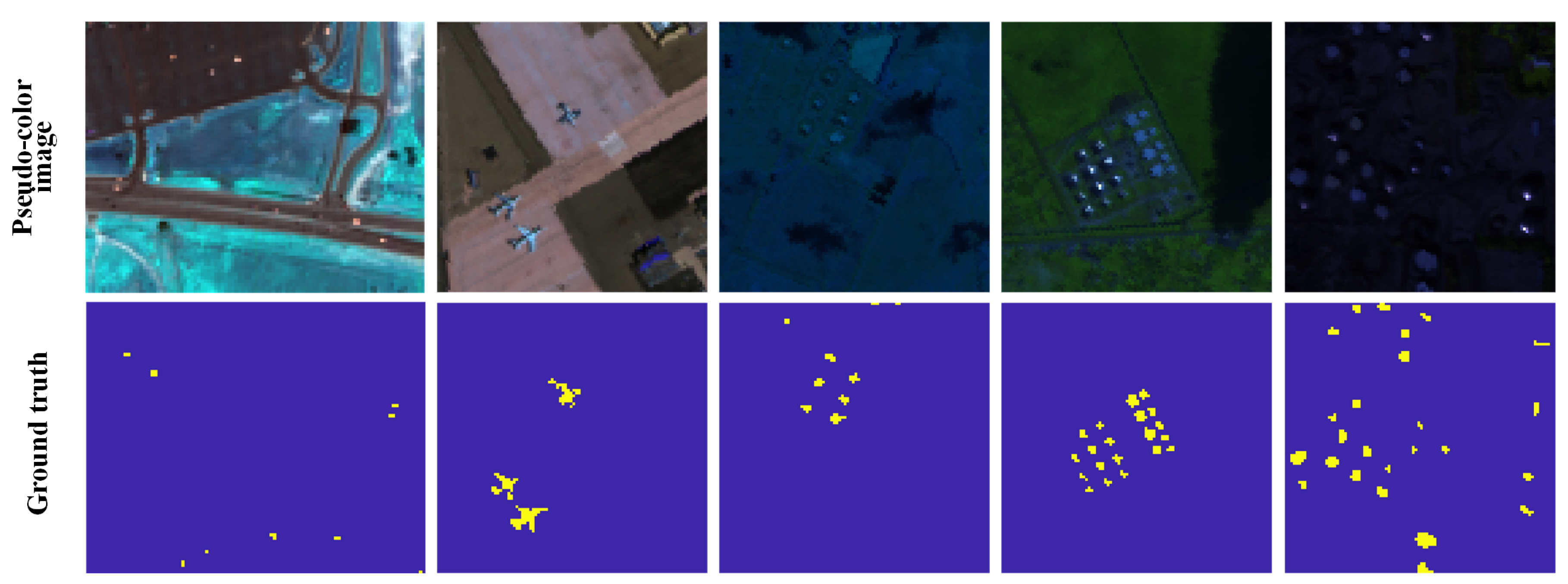
The first data set was recorded by the hyperspectral digital imagery collection experiment (HYDICE) sensor 1. It contains 162 bands after removing the noisy bands in a total of 210 bands with a sub-image of 80×100 for each band. Figure 2 (a). shows the pseudo-color image and ground truth.

4.1.2. San Diego Data Set

The second data set was captured by the Airborne Visible/Infrared Imaging Spectrometer (AVIRIS) sensor 2. After removing the water vapor absorption and low SNR bands, the sub-image is sliced from the original scene at the center of the original scene. The background contains hangars, parking aprons, and exposed soil. Figure 2 (b) shows the pseudo-color image and ground truth.

4.1.3. Texas Coast Data Set

The third and fourth data sets were acquired by the AVIRIS sensor. They were obtained from Airport-Beach-Urban (ABU) data sets with a series of scenes of the Texas Coast 3. Noisy bands in the original images have been removed. The first scene contains 100×100 pixels in the spatial domain with 204 bands. The second scene contains 100×100 pixels in the spatial domain with 207 bands. Figure 2 (c) and (d) show the pseudo-color image and ground truth.

4.1.4. Los Angeles Data Set

The fifth data set was also from ABU data sets and were captured by the AVIRIS sensor covering the Los Angeles city area with noisy bands in the original images being removed3. It contains 100×100 pixels in the spatial domain with 205 bands. Figure 2 (e) shows the pseudo-color image and ground truth.

4.2. Evaluation Indexes

Several metrics, i.e., the receiver operating characteristic (ROC) and the area under the curve (AUC), were leveraged for performance evaluation. Specifically, the 3D ROC curve of

(P_{D}, P_{F})

(P_{D}, τ)

, and

(P_{F}, τ)

was used to evaluate the detector effectiveness and the background suppression ability [2,3]. The

AU C_{BS}

is a measure that obtained by subtracting

AU C_{(F, τ)}

from

AU C_{(D, F)}

to describe the background suppression ability. The

AU C_{SNPR}

is a measure which is obtained by dividing

AU C_{(D, τ)}

AU C_{(F, τ)}

. It describes the signal-to-noise rate of the methods, where the false alarm probability can be assumed to be caused by noise. When the value is higher, the performance of the detector is better.

4.3. Implementation Details

Prior spectra in HSTD can be obtained by laboratory measurements or simulations. In this experiment, we obtain it by calculating the mean of the target spectra according to groundtruth. Compared to the commonly used optimization methods, such as Adagrad and Momentum optimization, the Adam algorithm is chosen for optimization with a better performance. The learning rate is set to 0.0001 and updated every 50 epochs. The normalization adopts batch normalization, and the momentum is set to 0.9. The mini-batch is a set amount of training samples that are less than the total training samples in the data set. In each iteration, the batch size of the network on a different set of samples is set to 32 until all of the samples are used in the data set. As the number of layers increases, the model does not show a noticeable accuracy increase because an over deep network leads to over-smoothing, thus leading to poor training accuracy. Accordingly, this work sets the depth to two layers: a balance of complexity and performance. For graph learning, the module converges when the interaction is 200. For the generative module, the training model parameters and checkpoint are saved every 200 iterations, and the number of cycles is adaptively determined in the test phase according to the detection accuracy.

4.4. Comparison Methods

For comparison, eight state-of-the-art methods were selected, i.e., CEM [7], ACE [13], hCEM [18], eCEM [19], CSCR [22], DSC [23], BLTSC [29], and WHTD [30]. All these methods were re-implemented according to the papers and open-source code. The AUC scores are listed in Table 2 to Table 6. According to them, the performance of the proposed model is superior to the compared methods in the

AU C_{SNPR}

and

AU C_{BS}

. The target detection and background suppression ability outperform other methods on most data sets.

4.5. Analysis of the Results

This section presents quantitative and qualitative experiments to validate the effectiveness of the proposed method. Performance evaluation includes 2D detection maps, 3D detection maps, 3D ROC analysis, and box-plot analysis, detailed as follows.

4.5.1. Quantitative Analysis

Table 2, Table 3, Table 4, Table 5, Table 6 and Table 7 show the assessment of different methods for different data sets through six different evaluation indexes.

Table 2. The Quantitative Results of the Compared and Proposed Methods on San Diego Data Set

Methods	$AU C_{(D, F)}$	$AU C_{(F, τ)}$	$AU C_{(D, τ)}$	$AU C_{BS}$	$AU C_{SNPR}$
ACE	0.97331	0.19440	0.46121	0.77891	2.37249
CEM	0.96615	0.03411	0.30351	0.93204	8.89861
eCEM	0.87246	0.00352	0.11064	0.86893	31.3964
hCEM	0.95866	0.12958	0.37872	0.82908	2.92266
BLTSC	0.96699	0.00211	0.14054	0.96488	66.7020
CSCR	0.90767	0.11453	0.24495	0.79313	2.13868
DSC	0.98846	0.00651	0.30534	0.98195	46.9101
WHTD	0.99286	0.00136	0.21972	0.99150	156.929
Proposed	0.99362	0.00062	0.06992	0.99300	112.597

Table 3. The Quantitative Results of the Compared and Proposed Methods on ABU-2 Data Set

Methods	$AU C_{(D, F)}$	$AU C_{(F, τ)}$	$AU C_{(D, τ)}$	$AU C_{BS}$	$AU C_{SNPR}$
ACE	0.73605	0.16987	0.36055	0.56618	2.12248
CEM	0.85598	0.01192	0.18881	0.84406	15.8347
eCEM	0.95001	0.00322	0.17984	0.94679	55.9387
hCEM	0.91435	0.10487	0.27172	0.80949	2.59111
BLTSC	0.87148	0.01332	0.19970	0.85816	14.9923
CSCR	0.97465	0.07370	0.35924	0.90095	4.87435
DSC	0.96575	0.00655	0.12170	0.95920	18.5749
WHTD	0.98099	0.00077	0.16159	0.98022	209.589
Proposed	0.99914	0.00057	0.05476	0.99857	96.0632

Table 4. The Quantitative Results of the Compared and Proposed Methods on ABU-3 Data Set

Methods	$AU C_{(D, F)}$	$AU C_{(F, τ)}$	$AU C_{(D, τ)}$	$AU C_{BS}$	$AU C_{SNPR}$
ACE	0.84312	0.15227	0.32359	0.69085	2.12513
CEM	0.86691	0.02227	0.20235	0.84464	9.08753
eCEM	0.88075	0.03513	0.17956	0.84562	5.11101
hCEM	0.96708	0.07389	0.23705	0.89319	3.20825
BLTSC	0.86691	0.00560	0.17108	0.86131	30.5505
CSCR	0.81881	0.04432	0.18554	0.77449	4.18647
DSC	0.93001	0.00067	0.01634	0.92933	24.2838
WHTD	0.98115	0.00154	0.16477	0.97961	107.271
Proposed	0.99487	0.00073	0.06572	0.99414	89.7801

Table 5. The Quantitative Results of the Compared and Proposed Methods on ABU-1 Data Set

Methods	$AU C_{(D, F)}$	$AU C_{(F, τ)}$	$AU C_{(D, τ)}$	$AU C_{BS}$	$AU C_{SNPR}$
ACE	0.95936	0.18326	0.46656	0.77610	2.54593
CEM	0.94110	0.01501	0.21594	0.92609	14.3842
eCEM	0.99025	0.03149	0.61422	0.95877	19.5076
hCEM	0.99164	0.15707	0.58292	0.83457	3.71131
BLTSC	0.94655	0.00499	0.17624	0.94156	35.2978
CSCR	0.99745	0.00309	0.05403	0.99436	17.4748
DSC	0.98754	0.02826	0.44433	0.95928	15.7235
WHTD	0.99694	0.00094	0.18216	0.99600	193.581
Proposed	0.99631	0.00036	0.11012	0.99595	309.312

Table 6. The Quantitative Results of the Compared and Proposed Methods on HYDICE Data Set

Methods	$AU C_{(D, F)}$	$AU C_{(F, τ)}$	$AU C_{(D, τ)}$	$AU C_{BS}$	$AU C_{SNPR}$
ACE	0.98642	0.24168	0.65020	0.74474	2.69031
CEM	0.98243	0.02187	0.44714	0.96056	20.4470
eCEM	0.98015	0.00298	0.16045	0.97717	53.8416
hCEM	0.99999	0.06944	0.56489	0.93055	8.13533
BLTSC	0.98243	0.01230	0.44536	0.97013	36.2108
CSCR	0.98648	0.00339	0.06766	0.98309	19.9416
DSC	0.92391	0.02961	0.15000	0.89429	5.06510
WHTD	0.99917	0.00131	0.39685	0.99786	305.308
Proposed	0.99986	0.00026	0.27252	0.99961	1060.39

Table 7. Average Scores of

AU C_{(D, F)}

AU C_{(F, τ)}

AU C_{BS}

, and

AU C_{SNPR}

for Compared Methods on Different Data Sets

Table 7. Average Scores of

AU C_{(D, F)}

AU C_{(F, τ)}

AU C_{BS}

, and

AU C_{SNPR}

for Compared Methods on Different Data Sets

ACE	CEM	eCEM	hCEM	BLTSC	CSCR	DSC	WHTD	Proposed	Improvement
0.89970	0.92250	0.93470	0.93500	0.92690	0.93700	0.95910	0.99020	0.99660	0.64633%
0.18830	0.02104	0.01527	0.04346	0.00766	0.04781	0.01432	0.00118	0.00078	33.8983%
0.71136	0.90148	0.91946	0.89156	0.91921	0.88920	0.94481	0.98904	0.99587	0.69057%
2.37127	13.7304	33.1591	56.6544	36.7507	9.72318	22.1115	194.535	333.629	71.5004%

For the HYDICE data set, although the proposed method has slightly lower detection accuracy than hCEM, its false alarm rate is one order of magnitude better than other methods, resulting in better

AU C_{SNPR}

and

AU C_{BS}

. So as on ABU-2 data set, the performance of the proposed method is comparable in

AU C_{(F, τ)}

AU C_{BS}

, and

AU C_{SNPR}

, which is mainly due to the different compensatory representation of the fusion network. For the San Diego data set, the

AU C_{(D, F)}

of the proposed method reaches 0.99362, and the

AU C_{BS}

of the proposed is 0.993, which is better than others. For ABU-2 and ABU-3 data sets, the proposed method performs well on most indexes, proving the effectiveness of graph and generative learning modules with frequency representation.

To provide a comprehensive performance comparison of the proposed algorithm, Table 7 calculates average scores for five real scene hyperspectral datasets, evaluating each method’s performance.

The proposed algorithm reaches the optimum on the average of

AU C_{(D, F)}

AU C_{(F, τ)}

AU C_{BS}

, and

AU C_{SNPR}

, which demonstrates better detection and background suppression ability.

4.5.2. Visual Analysis

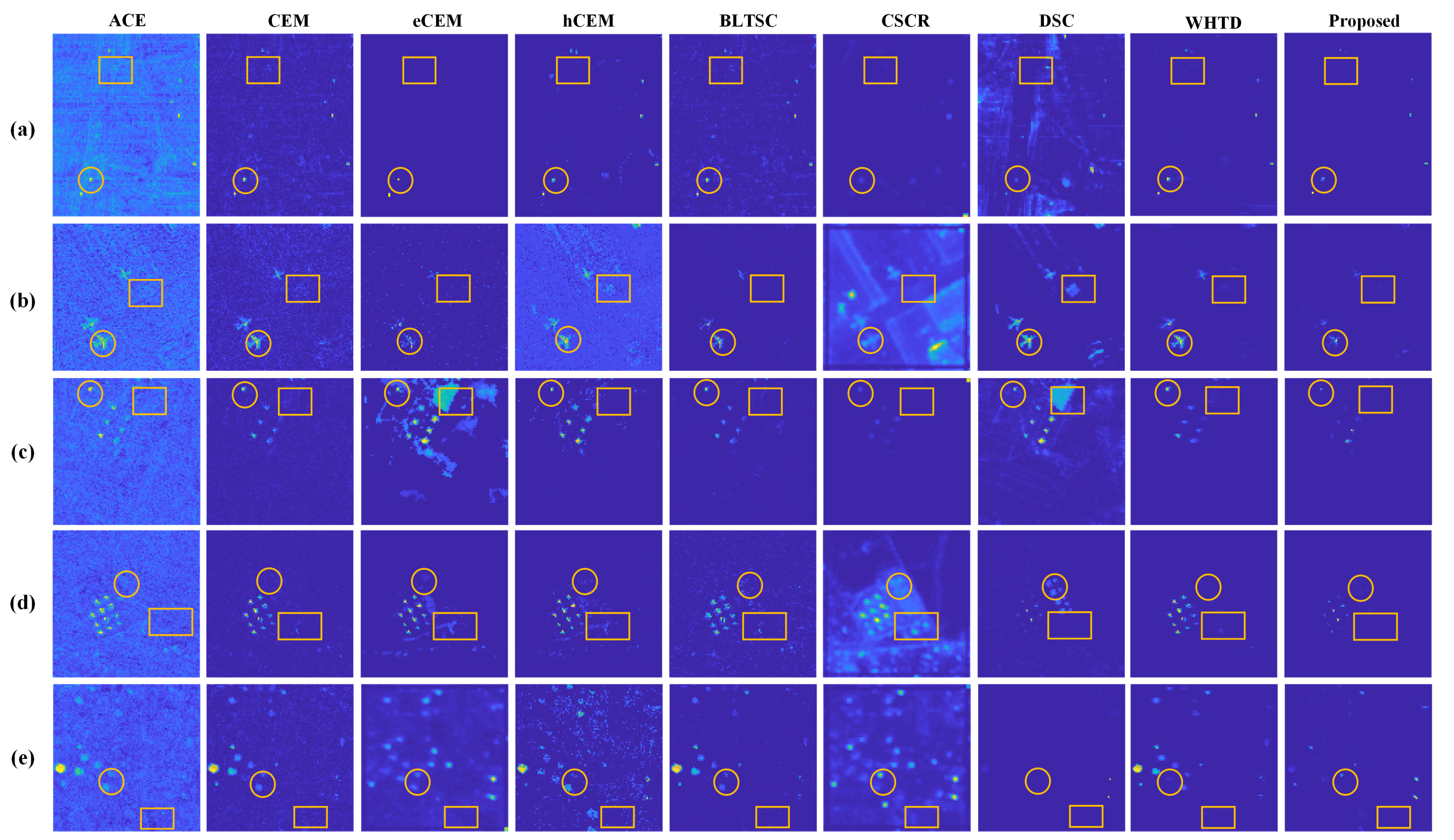
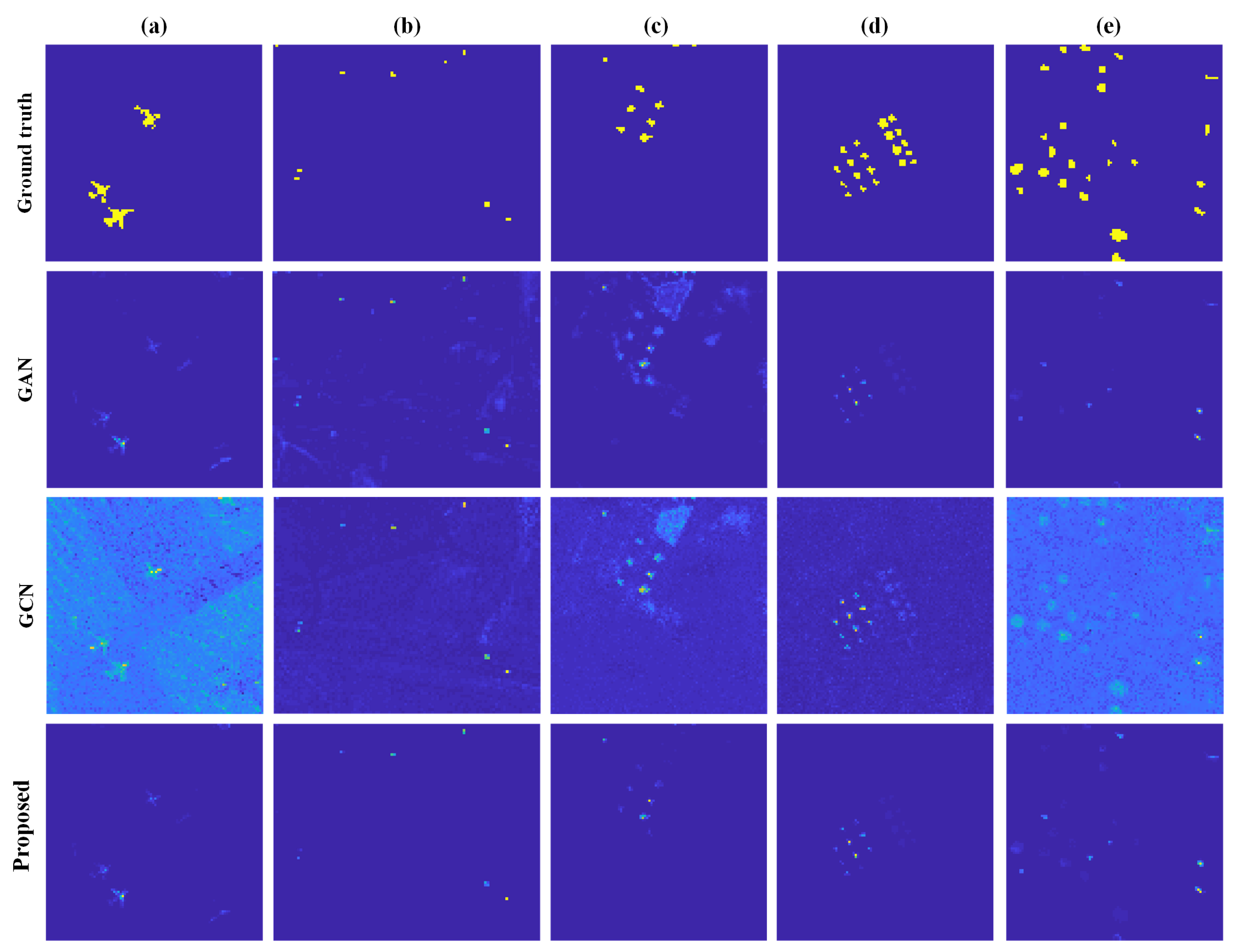
Figure 3 depicts the detection results of several approaches on diverse data sets. The targets and certain partial region around the targets are highlighted.

For HYDICE data sets, as shown in Figure 3 (a), the hCEM effectively decreases uniform background interference. However, there is blatant background noise interference around the target. Although there is some misdetection without background suppression and unstable performance in the CEM and CSCR methods, the recognition of structure and location is better. Despite some noise points in the background leading to occasional misidentifications in DSC, the method precisely locates targets. BLTSC rarely mistakes background for targets due to its background learning and spectral constraints. WHTD method, employing weakly supervised background estimation with target-based constraints and channel-wise attention, achieves clear and accurate target detection. The proposed method effectively detects targets and suppresses background, leveraging non-local and spectral-spatial information representation through the commentary architecture.

For the San Diego dataset, depicted in Figure 3 (b), eCEM and hCEM methods struggle with spectral variations in real scenes. The proposed detection map exhibits more precise and accurate target shapes, closely resembling ground truth as seen in BLTSC.

In the ABU-1 dataset Figure 3 (c), the proposed method achieves greater precision in target shape, with results closer to ground truth, featuring improved edge detection and smaller target recognition.

For ABU-2 Figure 3 (d), the proposed method focuses on accurate target detection while suppressing background interference. ACE and CEM methods identify fewer target pixels but demonstrate superior performance.

In Figure 3 (e), hCEM and DSC efficiently detect small targets in the ABU-3 dataset. The proposed method shows slightly blurred edges in detected targets but effectively suppresses background. Quantitative results align with findings from the 2D detection map.

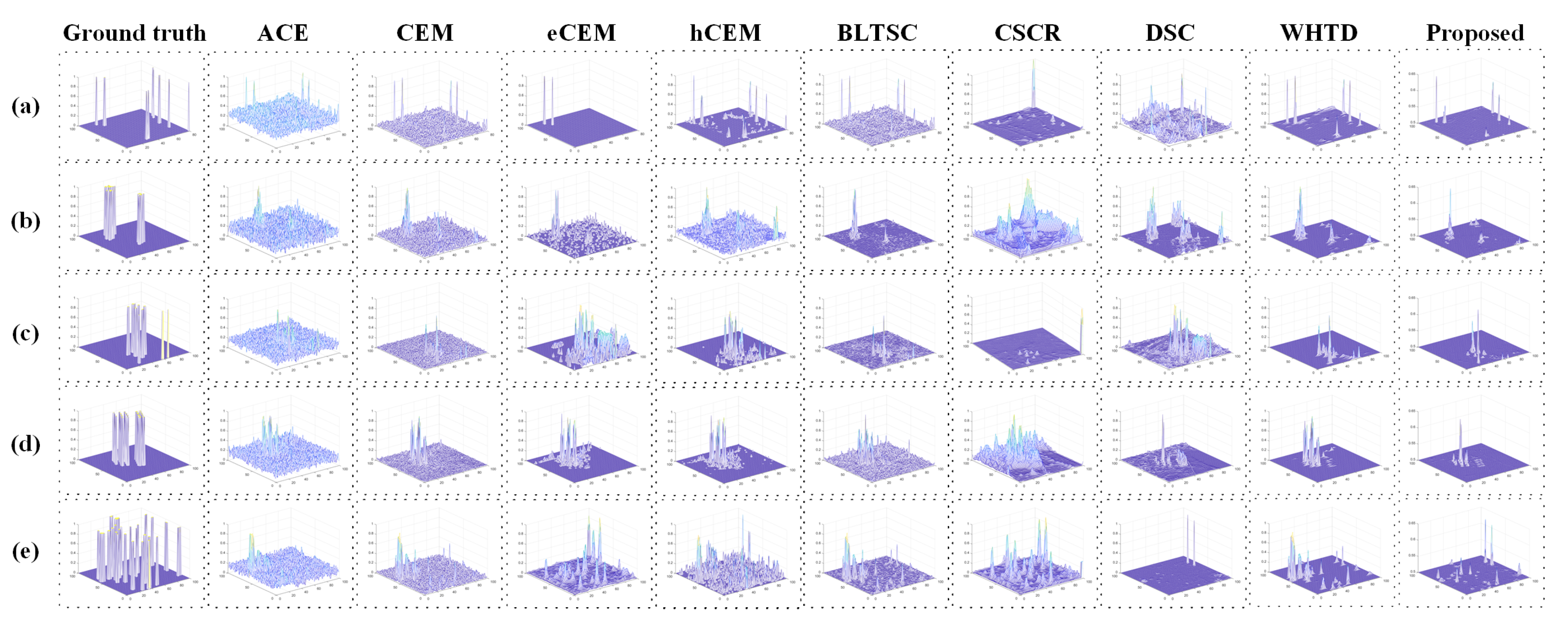
The corresponding 3D views of the detection results are depicted in Figure 5, demonstrating the background and target values and the discrimination visualization. The 2D and 3D results show that the proposed method performs better with more precise targets and lower background values in background suppression. This is mainly due to the compensation of both the GAN and GCN in feature extraction and representation ability to the detection. The hCEM, CSCR, and proposed method for the LA data set could maintain target morphology while attaining high detection values at target pixels.

4.5.3. 3D ROC Analysis

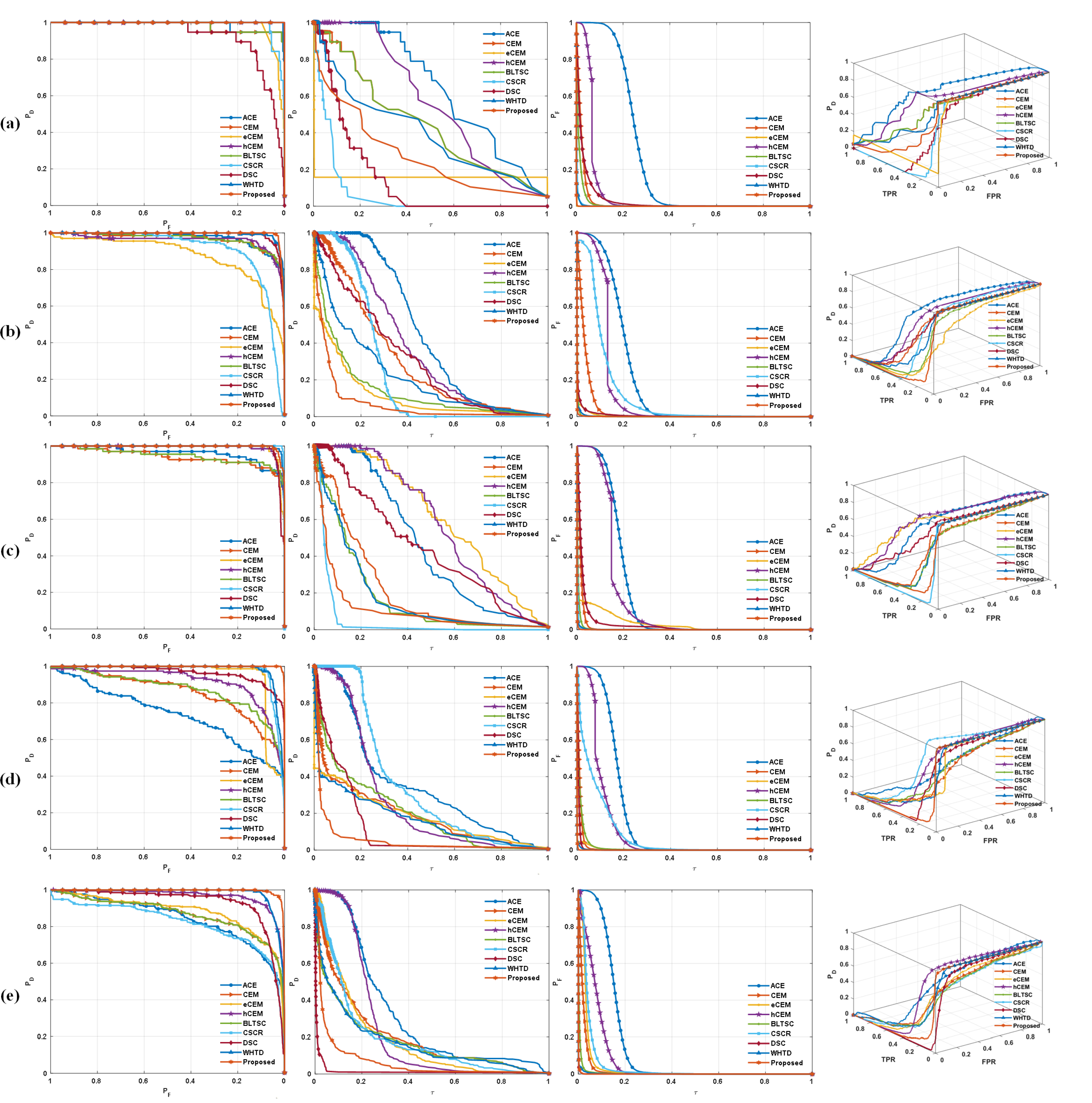
Figure 6 presents the 3D ROC of different methods on five data sets. When the ROC curves reach the upper range of the figure, the detector’s performance improves. The ROC curves of the proposed method surpass others for the San Diego data set. For HYDICE, the proposed method is above others in the low region. It is superior to others for ABU-1, ABU-2, and ABU-3 data sets. The hCEM is preferable to others in the high-

P_{F}

area, which is usually significant in practical applications. As ROC curves reach the upper limits, detector performance improves significantly. For the San Diego dataset, ROC curves of the proposed method outperform others. Higher values in these metrics indicate better detection performance. AUC of

(P_{F}, τ)

directly correlates with background suppression, with smaller values indicating superior performance. Similarly,

(P_{D}, P_{F})

assesses detector effectiveness under joint hypotheses

H_{0}

and

H_{1}

, while

(P_{D}, τ)

and

(P_{F}, τ)

characterize target detectability and background suppression under single hypotheses, respectively.

The AUC of

(P_{D}, P_{F})

and

(P_{D}, τ)

positively correlate with the detection performance. The higher the value of these two metrics, the better the detection performance. While the AUC of

(P_{F}, τ)

is directly related to background suppression performance, the smaller the value, the better the background suppression performance. So it can also represent good detection performance. The index negatively correlates with the detection performance.

(P_{D}, P_{F})

characterizes the effectiveness of the detector under the joint hypothesis

H_{0}

and

H_{1}

(P_{D}, τ)

is used to characterize target detectability under the single hypothesis

H_{1}

(P_{F}, τ)

was used to characterize the background suppression under the single hypothesis

H_{0}

Taking the ABU-1 data set as an example, in Figure 6, those different methods have different 3D ROC values. For the 2D ROC curve of

(P_{D}, P_{F})

, as the abscissa

P_{F}

increases, the ordinate

P_{D}

decreases accordingly. For the same

P_{F}

, the proposed algorithm has a smaller value of

P_{D}

than other algorithms. For the 2D ROC curve of

(P_{F}, τ)

, for the same

τ

, the proposed algorithm has a higher value of

P_{f}

than other algorithms, which reflects that the detection accuracy is higher under the same threshold. For the 2D ROC curve of

(P_{D}, τ)

, the proposed algorithm has a smaller value of

P_{D}

than other algorithms for the same

τ

, which reflects that the proposed algorithm has a fewer misdetection of targets with the same threshold. For the 3D ROC curve, the proposed algorithm achieves a higher curve value in the spatial dimension, meaning better detection performance.

4.5.4. Analysis of Contrast

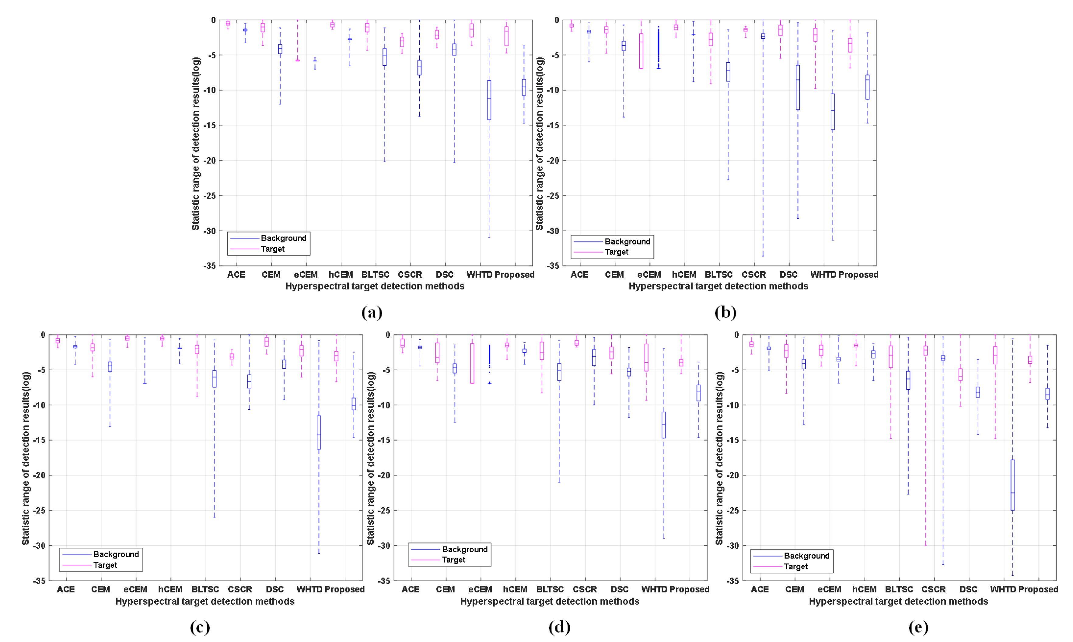
Figure 7 illustrates the proposed method’s separability abilities with a box plot figure. It can be observed from Figure 7 that the sparse contrast between the tiny target and the intricate background makes it challenging to gather accurate edge and shape information. In the proposed method, the target and background have a more aggregated concentration and a clear differentiation, respectively.

4.6. Ablation Study

Ablation studies evaluate GCN, GAN, fusion strategy, input frequency components, and small batch training patterns to assess their contributions to detection performance.

4.6.1. Analysis of graph and generative learning

Using graph and generative learning module compared to traditional detection have better performance. Table 8 shows the ablation study results of the two modules quantitatively. If we solely use GAN to locate targets, although possessing attractive detection precision, there is a higher false alarm rate. Moreover, in visual, some targets get lost in a cluttered background, which can be seen in Figure 8. Additionally, the incorporation of GCN enhances the precision of detection despite slight misdetection, as seen in Table 8.

For the ABU-2 dataset, the generative learning module enhances GCN performance significantly, while the fusion module marginally improves accuracy due to noise interference. Similar trends are observed in AUC indicators, reflecting the dataset’s susceptibility to surrounding noise. The generative network can better represent the spatial and spectral information, and the supplementary role of GCN to model the topological information is relatively tiny.

The false alarm rate for detecting discrete targets in the ABU-3 data set is relatively high, and GCN’s spectral distortion is severe. Therefore, the fused result improves the detection performance of GCN, but the generative network module works better. Meanwhile, the separation effect of GAN on the target and the background is also not significant, and the improvement of the fusion effect is limited. However, the generative learning module can also better model the spatial-spectral relationship, and the graph convolution module can detect the target’s spatial position.

For the HYDICE, San Diego, and ABU-1 data sets, the fusion improves the results of using only the graph or the generative modules. To summarize, each module impacts detection performance, and most of the combination provides beneficial outcomes, indicating how they supplement each other.

4.6.2. Analysis of Number of Training Samples

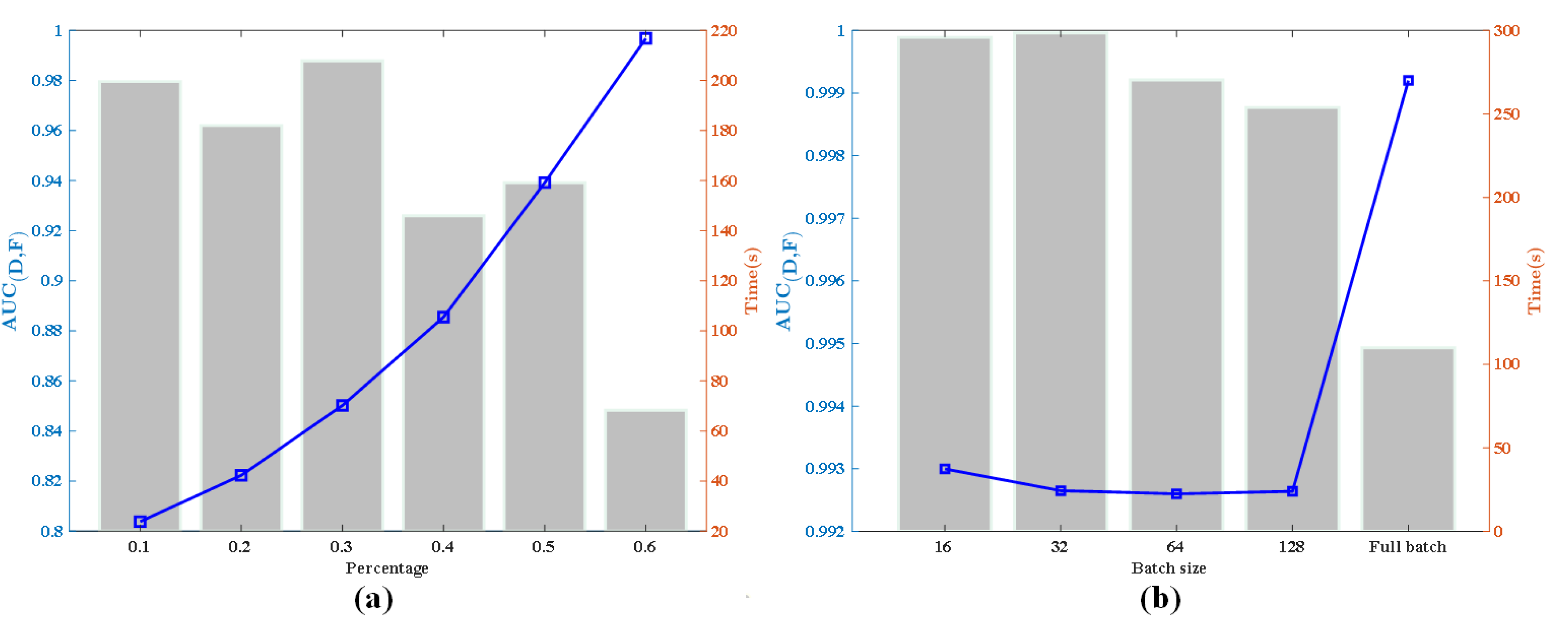
Across HYDICE, San Diego, and ABU-1 datasets, fusion improves results compared to using individual graph or generative modules. Exploration into sample size impact reveals optimal performance at 30% input, balancing indicator values and computational efficiency. Increasing sample size escalates computation time proportionally, underscoring the efficiency of small batch processing. To explore the impact of the input sample number, we input the training samples of different proportions into the GCN module. Table 9 shows that the input sample ratio has an impact on detection accuracy, false alarm rate, and calculation time. When the input percentage is 30%, the indicator value reaches a reasonable level, while the calculation time is not very high.

Figure 9 (a) shows the relationship between the percentage of input data with

AU C_{(D, F)}

and the relative running time. It can be observed that when the input sample ratio is changed, the accuracy varies between 0.8 and 1, and the accuracy reaches its best when it is 30%. The running time is proportional to the sample size, and as the number of samples increases, the running time shows a more noticeable increase trend. Therefore, we choose an appropriate proportion of input samples to balance accuracy and computational cost.

4.6.3. Effectiveness of Various Aggregations

In Table 10, different fusion strategies are compared to evaluate the effectiveness of the proposed fusion strategy.

As can be seen from Table 10, although the index of the proposed algorithm on

AU C_{(D, τ)}

and

AU C_{BS}

is slightly worse than the other two methods, it is better than additive fusion and dot production on

AU C_{(D, F)}

and

AU C_{(F, τ)}

. Therefore, the proposed fusion method proves to be more effective than addictive and dot production fusion.

4.6.4. Analysis of Small Batch Training Strategy

Figure 9 (b) shows the visualization of the relationship between

{AUC}_{(D, F)}

and batch size.

It can be seen from Figure 9 (b) that when the number of batches increases, the

AU C_{(D, F)}

does not vary a lot, but the consumption of computing resources is very different. When putting the whole batch into the network, the calculation time is several times that of the small batch. When the batch is set to 32, a balance is achieved between accuracy and running time. Table 11 shows that using a small batch pattern of GCN significantly improves computational time compared to the full batch.

5. Conclusion

In this article, we focus on the problem of low contrast and imbalance between the target and background, and the high computation cost caused by spatial redundancy with high spectral dimensions in target detection on HSIs. To solve the problems, we propose and investigate a deep representative learning model, a two-stream learning pattern consisting of the GCN and the GAN with feature compensation. In particular, the GCN and GAN modules capture and combine the irregular topological and spatial-spectral data to detect the small targets in HSIs. Moreover, the designed filter aggregates targets suppresses background, and generates pseudo labels for better results, as it enhances the targets. Experimental results on five different HSI data sets show that the proposed method performs better than other state-of-the-art methods, especially in background suppression ability.

Author Contributions

Methodology, L. Y., Z. J., and X. W.; software, Z. J., X. W., and G. P.; formal analysis, L. Y.; X. W.; G. P; writing—original draft preparation, Z. J.; supervision, L. Y.; X. W.; G. P. All authors have read and agreed to the published version of the manuscript.

Funding

This work was supported in part by the National Natural Science Foundation of China under Grant No. 62121001 and Grant No. U22B2014; in part by Young Elite Scientist Sponsorship Program by the China Association for Science and Technology under Grant 2020QNRC001; in part by China Scholarship Council No. 202206960021.

Data Availability Statement

The original data presented in the study are included in the article, and are also available from the corresponding author.

Acknowledgments

Thanks to the researchers who provided the experimental data and comparison methods.

Conflicts of Interest

The authors declare no conflicts of interest.

References

Chang, C.; Ren, H.; Chiang, S. Real-Time Processing Algorithms for Target Detection and Classification in Hyperspectral Imagery. IEEE Trans. Geosci. Remote Sens. 2001, 39, 760–768. [Google Scholar] [CrossRef]
Chang, C. Hyperspectral Target Detection: Hypothesis Testing, Signal-to-Noise Ratio, and Spectral Angle Theories. IEEE Trans. on Geosci. and Remote Sens. 2021, 60, 1–23. [Google Scholar] [CrossRef]
Chang, C. An Effective Evaluation Tool for Hyperspectral Target Detection: 3D Receiver Operating Characteristic Curve Analysis. IEEE Trans. on Geosci. and Remote Sens. 2020, 59, 5131–5153. [Google Scholar] [CrossRef]
Manolakis, D. Taxonomy of Detection Algorithms for Hyperspectral Imaging Applications. Opt. Eng. 2005, 44, 066403–066403. [Google Scholar] [CrossRef]
Li, Y.; Shi, Y.; Wang, K.; Xi, B.; Li, J.; Gamba, P. Target Detection with Unconstrained Linear Mixture Model and Hierarchical Denoising Autoencoder in Hyperspectral Imagery. IEEE Trans. on Image Process. 2022, 31, 1418–1432. [Google Scholar] [CrossRef] [PubMed]
Yao, C.; Yuan, Y.; Jiang, Z. Self-Supervised Spectral Matching Network for Hyperspectral Target Detection. Proc. IEEE Int. Geosci. Remote Sens. Symp. (IGARSS) 2021, 2524–2527. [Google Scholar]
Chang, C. Hyperspectral Data Processing: Algorithm Design and Analysis. John Wiley & Sons, 2013. [Google Scholar]
Rao, W.; Gao, L.; Qu, Y.; Sun, X.; Zhang, B.; Chanussot, J. Siamese Transformer Network for Hyperspectral Image Target Detection. IEEE Trans. on Geosci. and Remote Sens. 2022, 60, 1–19. [Google Scholar] [CrossRef]
Harsanyi, J.; Chang, C. Hyperspectral Image Classification and Dimensionality Reduction: An Orthogonal Subspace Projection Approach. IEEE Trans. on Geosci. and Remote Sens. 1994, 32, 779–785. [Google Scholar] [CrossRef]
Kraut, S.; Louis, L.; Ronald, W. Adaptive subspace detectors. IEEE Trans. Signal Process. 2001, 49, 3005–3014. [Google Scholar] [CrossRef]
Yang, S.; Shi, Z. SparseCEM and SparseACE for Hyperspectral Image Target Detection. IEEE Geosci. and Remote Sens. Lett. 2014, 11, 2135–2139. [Google Scholar] [CrossRef]
Chen, L.; Liu, J.; Sun, S.; Chen, W.; Du, B.; Liu, R. An Iterative GLRT for Hyperspectral Target Detection Based on Spectral Similarity and Spatial Connectivity Characteristics. IEEE Trans. on Geosci. and Remote Sens. 2023, 61, 1–11. [Google Scholar] [CrossRef]
Kraut, S.; Louis, L.; Ronald, W. The Adaptive Coherence Estimator: a Uniformly Most-Powerful-Invariant Adaptive Detection Statistic. IEEE Trans. on Signal Process. 2005, 53, 427–438. [Google Scholar] [CrossRef]
Robey, F.; Fuhrmann, D.; Kelly, E.; Nitzberg, R. A CFAR Adaptive Matched Filter Detector. IEEE Trans. Aerosp. Electron. Syst. 1992, 28, 208–216. [Google Scholar] [CrossRef]
Kraut, S.; Scharf, L. The CFAR Adaptive Subspace Detector is a Scale-Invariant GLRT. IEEE Trans. on Signal Process. 1999, 47, 2538–2541. [Google Scholar] [CrossRef]
J. C. Harsanyi. Detection and classification of subpixel spectral signatures in hyperspectral image sequences. Ph.D. dissertation 1993. [Google Scholar]
W. Farrand. Mapping the distribution of mine tailings in the Coeurd’Alene River Valley, Idaho, through the use of a constrained energy minimization technique. Remote Sens. Environ. 1997, 59, 64–76. [Google Scholar] [CrossRef]
Zou, Z.; Shi, Z. Hierarchical Suppression Method for Hyperspectral Target Detection. IEEE Trans. on Geosci. and Remote Sens. 2015, 54, 330–342. [Google Scholar] [CrossRef]
Zhao, R.; Shi, Z.; Zou, Z.; Zhang, Z. Ensemble-based Cascaded Constrained Energy Minimization for Hyperspectral Target Detection. Remote Sens. 2019, 11, 1310. [Google Scholar] [CrossRef]
Yang, X.; Jie, C.; Zhe, H. Sparse-Spatial CEM for Hyperspectral Target Detection. IEEE J. Sel. Top Appl. Earth. Obs. Remote Sens. 2019, 12, 2184–2195. [Google Scholar] [CrossRef]
Zhu, D.; Du, B.; Zhang, L. Single-Spectrum-Driven Binary-Class Sparse Representation Target Detector for Hyperspectral Imagery. 59 2020, 59, 1487–1500. [Google Scholar] [CrossRef]
Li, W.; Du, Q.; Zhang, B. Combined Sparse and Collaborative Representation for Hyperspectral Target Detection. Pattern Recognit. 2015, 48, 3904–3916. [Google Scholar] [CrossRef]
Shen, D.; Ma, X.; Wang, H.; Liu, J. A Dual Sparsity Constrained Approach for Hyperspectral Target Detection. The International Geoscience and Remote Sensing Symposium 2022 (IGARSS2022), Kuala Lumpur, Malaysia, 17-22 July, 2022, 1963–1966.
Jiao, C.; Yang, B.; Liu, L.; Chen, C.; Chen, X.; Yang, W.; Jiao, L. Semantic Modeling of Hyperspectral Target Detection with Weak Labels. Signal Process. 2023, 209, 109016. [Google Scholar] [CrossRef]
Kwon, H.; Nasrabadi, N. Kernel Spectral Matched Filter for Hyperspectral Imagery. Int. J. Comput. Vis. 2007, 71, 127–141. [Google Scholar] [CrossRef]
Wang, Y.; Chen, X.; Wang, F.; Song, M.; Yu, C. Meta-Learning Based Hyperspectral Target Detection Using Siamese Network. IEEE Trans. on Geosci. and Remote Sens. 2022, 60, 1–13. [Google Scholar] [CrossRef]
Xie, W.; Yang, J.; Lei, J.; Li, Y.; Du, Q.; He, G. SRUN: Spectral Regularized Unsupervised Networks for Hyperspectral Target Detection. IEEE Trans. on Geosci. and Remote Sens. 2020, 58, 1463–1474. [Google Scholar] [CrossRef]
Shi, Y.; Li, J.; Zheng, Y.; Xi, B.; Li, Y. Hyperspectral Target Detection with RoI Feature Transformation and Multiscale Spectral Attention. IEEE Trans. on Geosci. and Remote Sens. 2021, 59, 5071–5084. [Google Scholar] [CrossRef]
Xie, W.; Zhang, X.; Li, Y.; Wang, K.; Du, Q. Background Learning Based on Target Suppression Constraint for Hyperspectral Target Detection. IEEE J. Sel. Top Appl. Earth. Obs. Remote Sens. 2020, 13, 5887–5897. [Google Scholar] [CrossRef]
Qin, H.; Xie, W.; Li, Y.; Jiang, K.; Lei, J.; Du, Q. Weakly Supervised Adversarial Learning via Latent Space for Hyperspectral Target Detection. Pattern Recognit. 2023, 135, 109125. [Google Scholar] [CrossRef]
Kipf, T.; Welling, M. Semi-Supervised Classification with Graph Convolutional Networks. arXiv preprint arXiv:1609.02907, arXiv:1609.02907 2016.
Wu, Z.; Pan, S.; Chen, F.; Long, G.; Zhang, C.; Philip, S. A Comprehensive Survey on Graph Neural Networks. IEEE Trans. Neural Netw. Learn. Syst. 2020, 32, 4–24. [Google Scholar] [CrossRef]
Hong, D.; Gao, L.; Yao, J.; Zhang, B.; Plaza, A.; Chanussot, J. Graph Convolutional Networks for Hyperspectral Image Classification. IEEE Trans. on Geosci. and Remote Sens. 2020, 59, 5966–5978. [Google Scholar] [CrossRef]
Dong, Y.; Liu, Q.; Du, B.; Zhang, L. Weighted Feature Fusion of Convolutional Neural Network and Graph Attention Network for Hyperspectral Image Classification. IEEE Trans. on Image Process. 2022, 31, 1559–1572. [Google Scholar] [CrossRef] [PubMed]
Dong, Y.; Shi, W.; Du, B.; Hu, X.; Zhang, L. Asymmetric Weighted Logistic Metric Learning for Hyperspectral Target Detection. IEEE Trans. Cybern. 2021, 52, 11093–11106. [Google Scholar] [CrossRef] [PubMed]
Xu, Y.; Du, B.; Zhang, L. Robust Self-Ensembling Network for Hyperspectral Image Classification. IEEE Trans. Neural Netw. Learn. Syst. 2022. [Google Scholar] [CrossRef] [PubMed]
Xu, K.; Qin, M.; Sun, F.; Wang, Y.; Chen, Y.; Ren, F. Learning in the Frequency Domain. IEEE/CVF Conference on Computer Vision and Pattern Recognition (CVPR2022), Seattle, WA, USA, –19 2020. 13 June.
Takikawa, T.; Acuna, D.; Jampani, V.; Fidler, S. Gated-scnn: Gated Shape CNNs for Semantic Segmentation. IEEE/CVF International Conference on Computer Vision (ICCV), Seoul, Korea (South), Oct. 27–Nov. 2, 2019; pp. 5229–5238.
Bo, D.; Wang, X.; Shi, C.; Shen, H. Beyond Low-Frequency Information in Graph Convolutional Networks. AAAI Conference on Artificial Intelligence (AAAI-21), virtually, -9, 2021; pp. 3950–3957. 2 February.
Niepert, M.; Ahmed, M.; Kutzkov, K. Learning Convolutional Neural Networks for Graphs. Proceedings of the 33nd International Conference on Machine Learning (ICML), New York City, NY, USA, -24, 2016; pp. 2014–2023. 19 June.
Zeng, H.; Zhou, H.; Srivastava, A.; Kannan, R.; Prasanna, V. Graphsaint: Graph Sampling Based Inductive Learning Method. arXiv preprint, 2019; arXiv:1907.04931. [Google Scholar]

1	http://www.erdc.usace.army.mil/Media/FactSheets/FactSheetsArticleView/tabid/9254/Article/476681/hypercube
2	http://aviris.jpl.nasa.gov/
3	http://xudongkang.weebly.com/

Figure 1. Graphical representation of the flowchart of the proposed method, comprising four major modules: 1) a graph learning module, 2) a generative learning module, 3) a frequency representation module, and 4) a fusion module. The first module extracts the underlying data properties from the original HSI, while the second provides complementary spectral and spatial characteristics. The frequency learning module is added before training to achieve the frequency representation of the component through analyzing the spectral properties of HSIs to extract relevant features. Finally, the fusion module integrates the two modules to achieve a more abundant feature extraction and information aggregation.

Figure 2. The pseudo color image and ground-truth for the (a) HYDICE. (b) San Diego. (c) ABU-1. (d) ABU-2. (e) ABU-3.

Figure 3. The visual detection results of different detectors for the (a) HYDICE. (b) San Diego. (c) ABU-1. (d) ABU-2. (e) ABU-3.

Figure 4. Local detailed detection map of the HYDICE data set.

Figure 5. The 3D detection maps of different detectors for the (a) HYDICE. (b) San Diego. (c) ABU-1. (d) ABU-2. (e) ABU-3.

Figure 6. The 3D ROC curves of different detectors on (a) HYDICE. (b) San Diego. (c) ABU-1. (d) ABU-2. (e) ABU-3.

Figure 7. The separability analysis of different detectors on (a) HYDICE. (b) San Diego. (c) ABU-1. (d) ABU-2. (e) ABU-3.

Figure 8. Component analysis for the (a) HYDICE. (b) San Diego. (c) ABU-1. (d) ABU-2. (e) ABU-3.

Figure 9. Effects of input samples and batch size with

{AUC}_{(D, F)}

and computational cost.

Figure 9. Effects of input samples and batch size with

{AUC}_{(D, F)}

and computational cost.

Table 1. Descriptions of the Data Sets

Details	HYDICE	San Diego	Texas Coast-1	Texas Coast-2	Los Angeles
Sensor	HYDICE	AVIRIS	AVIRIS	AVIRIS	AVIRIS
Image size	[80,100]	[100,100]	[100,100]	[100,100]	[100,100]
Bands	162	189	204	207	205
Target type	cars,roofs	aircrafts	buildings	buildings	storage tank
Target pixels	19	134	67	155	272
Proportion	2.38%	1.34%	0.67%	1.55%	2.72%
Background type	vegetation area	San Diego airport	urban area	urban area	urban area
Captured place	California	California	Texas Coast	Texas Coast	Los Angeles
Flight time	1990s	11/16/2011	8/29/2010	8/29/2010	11/9/2011
SpeR	10nm	10nm	10nm	10nm	10nm
SpaR	1.56 m	3.5m	17.2m	17.2m	7.1m
SpeRange	400-2500	370-2510	450-1350	450-1350	430-860

Table 8. Ablation Comparison of each Module on Five Data Sets

Dataset	Methods	$AU C_{(D, F)}$	$AU C_{(F, τ)}$	$AU C_{(D, τ)}$	$AU C_{BS}$	$AU C_{SNPR}$
	Graph	0.99972	0.02280	0.47336	0.97692	20.7651
HYDICE	Generative	0.99895	0.00764	0.40712	0.99131	53.3230
	Proposed	0.99986	0.00026	0.27252	0.99961	1060.39
	Graph	0.91081	0.25967	0.42753	0.65114	1.64648
San Diego	Generative	0.99225	0.00125	0.08267	0.99100	66.3992
	Proposed	0.99362	0.00062	0.06992	0.99300	112.597
	Graph	0.99053	0.05121	0.35167	0.93933	6.86739
ABU-1	Generative	0.99290	0.00676	0.22824	0.98614	33.7485
	Proposed	0.99631	0.00036	0.11012	0.99595	309.312
	Graph	0.94012	0.02563	0.15867	0.91448	6.18975
ABU-2	Generative	0.99914	0.00013	0.05457	0.99901	433.095
	Proposed	0.99914	0.00057	0.05476	0.99857	96.0632
	Graph	0.96671	0.13761	0.31746	0.82911	2.30702
ABU-3	Generative	0.99508	0.00016	0.04175	0.99491	256.129
	Proposed	0.99487	0.00073	0.06572	0.99414	89.7801

Table 9. Ablation Study of the Impact of Input Samples Percentage on ABU-3 Data Set

Samples	$AU C_{(D, F)}$	$AU C_{(F, τ)}$	$AU C_{(D, τ)}$	$AU C_{BS}$	$AU C_{SNPR}$	Time (s)
10%	0.97957	0.05774	0.19019	0.92183	3.29370	23.8115
20%	0.96201	0.22954	0.46994	0.73247	2.04731	42.3048
30%	0.98781	0.02690	0.11420	0.96091	4.24512	70.2085
40%	0.92593	0.30465	0.57409	0.62128	1.88446	105.489
50%	0.93916	0.21722	0.36985	0.72193	1.70263	159.189
60%	0.84830	0.06381	0.15778	0.78449	2.47280	216.796

Table 10. Ablation Study of the Impact of Fusion Strategy on ABU-3 Data Set

Method	$AU C_{(D, F)}$	$AU C_{(F, τ)}$	$AU C_{(D, τ)}$	$AU C_{BS}$	$AU C_{SNPR}$
Additive Fusion	0.91576	0.00054	0.05422	0.91522	99.8527
Dot Production	0.99140	0.27241	0.39487	0.71899	1.44953
Proposed	0.99487	0.00073	0.06572	0.99414	89.7801

Table 11. Ablation Study of the Impact of Batch Size on HYDICE Data Set

Batch size	$AU C_{(D, F)}$	$AU C_{(F, τ)}$	$AU C_{(D, τ)}$	$AU C_{BS}$	$AU C_{SNPR}$	Time (s)
16	0.99989	0.00148	0.34993	0.99841	236.117	37.3738
32	0.99996	0.00027	0.28358	0.99969	1038.75	24.3253
64	0.99921	0.00279	0.33924	0.99642	121.504	22.4265
128	0.99877	0.00343	0.40135	0.99534	117.046	23.9302
Full batch	0.99493	0.00530	0.36743	0.98963	69.3387	270.052

Disclaimer/Publisher’s Note: The statements, opinions and data contained in all publications are solely those of the individual author(s) and contributor(s) and not of MDPI and/or the editor(s). MDPI and/or the editor(s) disclaim responsibility for any injury to people or property resulting from any ideas, methods, instructions or products referred to in the content.

© 2024 by the authors. Licensee MDPI, Basel, Switzerland. This article is an open access article distributed under the terms and conditions of the Creative Commons Attribution (CC BY) license (http://creativecommons.org/licenses/by/4.0/).

Copyright: This open access article is published under a Creative Commons CC BY 4.0 license, which permit the free download, distribution, and reuse, provided that the author and preprint are cited in any reuse.

MDPI Initiatives

Important Links

Choose an area of interest and we will send you notifications of new preprints at your preferred frequency.

Disclaimer

Representation Learning-Based Graph and Generative Network for Hyperspectral Small Target Detection

Abstract

1. Introduction

2. Graph Learning

3. Proposed Methodology

3.1. Overall Framework

3.2. Data Preparation based on Frequency Learning

3.3. The Graph Learning Module

3.4. Generative Learning Module

3.5. Fusion and Aggregation Module

4. Experimental Results and Analysis

4.1. Data Sets

4.1.1. HYDICE Data Set

4.1.2. San Diego Data Set

4.1.3. Texas Coast Data Set

4.1.4. Los Angeles Data Set

4.2. Evaluation Indexes

4.3. Implementation Details

4.4. Comparison Methods

4.5. Analysis of the Results

4.5.1. Quantitative Analysis

4.5.2. Visual Analysis

4.5.3. 3D ROC Analysis

4.5.4. Analysis of Contrast

4.6. Ablation Study

4.6.1. Analysis of graph and generative learning

4.6.2. Analysis of Number of Training Samples

4.6.3. Effectiveness of Various Aggregations

4.6.4. Analysis of Small Batch Training Strategy

5. Conclusion

Author Contributions

Funding

Data Availability Statement

Acknowledgments

Conflicts of Interest

References

MDPI Initiatives

Important Links

Subscribe