Preprint
Article

A-optimal Designs of High-Order Mixture Central Polynomial Model

Altmetrics

Downloads

88

Views

30

Comments

0

This version is not peer-reviewed

Submitted:

27 July 2024

Posted:

30 July 2024

You are already at the latest version

Alerts
Abstract
This article systematically studied the A-optimal designs of a high-order mixture central polynomial model, which is an advancement of the research results for the A-optimal design of the most recent third-order mixture central polynomial model and a more accurate response surface model. This article is based on the simplex center design, obtaining measurement values at various design points, and verifying them through the A-optimal equivalence theorem. We also compare the A-efficiency of designs through examples, which can be applied to the A-optimal precise design of the fourth-order mixture model.
Keywords: 
Subject: Computer Science and Mathematics  -   Probability and Statistics

1. Introduction

Mixture experiment design is commonly used in the medical, biological, chemical, pharmaceutical, and consumer goods industries [1]. Usually in mixture tests, the reaction is only related to the proportion of the mixture components, not the amount of the mixture.
The foundational work of mixture material experimental design was Scheffé [2] study on the simplex lattice design and simplex center design of the mixture material specification polynomial model. The Research on optimal design can be roughly divided into four aspects: (a) research on optimal design of various commonly used models; (b) research on optimal design under constraints or additional conditions; (c) research on optimal design algorithms; and (d) research on applications. In recent years, the optimal design of mixture experiments has been widely applied.
The latest research results, Research results on (a), include the I-optimal design of the Scheffé mixture model studied by Goos et al. [3]. Hao et al. [4] studied the R-optimal design of second-order Scheffé mixture models and obtained a general expression for the measure. Research progress has also been made on the R-optimal design of other models and problems [5,6,7,8]. Jiang et al. [9] studied the K-optimal design of second-order mixture material models, expanding research on multiple response problems in various models and designs [10,11]. Dette, Liu, and Yue studied design admissibility and the de la Garza phenomenon in multifactor experiments [12]. Research results on (b), Leng and Yin [13] studied the Bayesian optimal design of multi-factor additive nonlinear models using the second-order least squares method, Chen et al. [14] studied the D- and A-optimal designs of multi-response mixture experiments with qualitative factors and Li et al. [15] studied the optimal design of uncertain response mixture models. Research results on (c), the algorithm has been improved, such as the the directional graph sequential design algorithm for simplex center design [16], the threshold acceptance algorithm [17], the improved DE algorithm [18], and the random search algorithm [19]. Regarding (d), Goos studied fish patty using a strip-plot designed for mixed material experiments [20]. Goos and Hamidouche [21] used a mixture choice model to study the cocktail.
Regarding A-optimal design, Chen [22] summarized the research results and solved linear and second-order central polynomial models, whereas Zhu and Hao [23] studied A-optimal design for special third-order mixture models. This article further addresses the complex but highly accurate fourth-order model. Other studies on A-optimal design include Chan et al. [24] studying second-order additive models and Zhu et al. [25] studying A-optimal design for mixture central polynomial models with qualitative factors. Li and Zhang [26] introduced the A-optimal design of a second-order polynomial mixture model with splines, Chen et al. [14] studied the A-optimal design of multi-response mixture models with qualitative factors, and Yan et al. [27] studied the mixture polynomial model with heteroscedasticity. Pal et al. [28] studied A-optimal designs for optimum mixture in an additive quadratic mixture model.
This article introduces the basic concept of the mixture model in Section 1, the A-optimal design criterion in Section 2, and the A-optimal design of the fourth-order mixture model in Section 3, which is the main work of the paper. We provide measures for the A-optimal design of the fourth-order mixture model at various experimental design points, and verify that the fourth-order mixture central polynomial model satisfies the equivalence theorem of A-optimal design. In the final section of this article, the main results are summarized.

2. Model and Design

This section introduces the mixture model studied in this article and introduces design-oriented concepts.

2.1. Mixture Model

The variables in the mixture model refer to the proportion of each component in the total mixture amount, independent of the total amount. Assuming that x i component variables are denoted as i = 1 , 2 , 3 , , q and satisfy i = 1 q x i = 1 , this constraint is called the basic mixture constraint. The experimental domain of mixture materials without additional constraints can be represented as S q 1 = { ( x 1 , x 2 , , x q ) : i = 1 q x i = 1 , 0 x i 1 , i = 1 , 2 , , q } , which is called a q 1 -dimensional normal simplex.
The general linear regression model in the experimental domain is y ( x ) = β T F ( x ) + ϵ , where y ( x ) is the observed value of the response at test point x, F ( x ) = ( f 1 ( x ) , f 2 ( x ) , , f p ( x ) ) T is the column vector of the variables given p continuous functions about point x = ( x 1 , x 2 , , x q ) S q 1 , ϵ N ( 0 , σ 2 ) , and β = ( β 1 , β 2 , , β p ) T is the estimated parameter vector, represented by η as the response. This model is often referred to as η ( x ) = β T F ( x ) = F T ( x ) β .
The mixture material model is different from general regression models due to the experimental domain. Scheffé pioneered the Scheffé canonical polynomial model, which emphasizes practicality, simplifies the model, reduces design points, and can also create a mixture material center multi term model based on effectively fitting the response surface. It is also the model used in this study, specifically:
η = i = 1 q β i x i + i < j β i j x i x j + i < j < k β i j k x i x j x k + i < j < k < l x i x j x k x l ,
Abbreviated as η = f T ( x ) β , among f ( x ) = ( x 1 , x 2 , , x q , x 1 x 2 , x 1 x 3 , , x q 1 x q , x 1 x 2 x 3 , , x q 3 x q 2 x q 1 x q ) T , β = ( β 1 , β 2 , , β q , β 12 , β 13 , , β q 1 , q , β 123 , , β q 3 , q 2 , q 1 , q ) , both f ( x ) and β are p = 2 q 1 are C q + m 1 m -dimensional column vectors, which reduces the number to many terms compared to the m order normal polynomial model and is more conducive to estimating model parameters with very few design points.

2.2. Design

For Model (1) to estimate by arranging design points, the experimental design is any probability distribution on the experimental domain, denoted as continuous design ξ as:
ξ = x 1 x 2 x n ω 1 ω 2 ω n ,
where there are n non repeating design points x i ( i = 1 , 2 , , n ) , each given a measure ω i , which has i = 1 n ω i = 1 . However, exact design is a design that specifies the total number of trials as N and provides N replicable design points. Let all members of this type of design be denoted as Ξ . For Design 2, its information matrix is defined as:
M ( ξ ) = S q 1 f ( x ) f T ( x ) d ξ ( x ) ,
and the information matrix is non-singular. The purpose of A-optimal design is to find a design ξ in the real functional Φ of M ( Ξ ) based on the A-optimal criterion.
The simplex center design is the basic design of the mixture experiment, and the number of polynomial model parameters for the q component mixture center is consistent with the number of simplex center design points. Therefore, the simplex center design is also a saturated design. The set of design points for the center of the q component simplex is denoted as { q , q } , where the first q is the q component and the second q is the q order. For example, in point set { 3 , 3 } , which is a three component, three-order simplex center design, there are three pure component mixture experimental design points { 1 , 0 , 0 } , { 0 , 1 , 0 } , { 0 , 0 , 1 } ; design point { 1 / 2 , 1 / 2 , 0 } , { 1 / 2 , 0 , 1 / 2 } , { 0 , 1 / 2 , 1 / 2 } for three two-component mixture tests; and design point { 1 / 3 , 1 / 3 , 1 / 3 } for a three-component mixture test. For the four-component, four-order simplex center design { 4 , 4 } studied in this article, there are four pure component points { 1 , 0 , 0 , 0 } , { 0 , 1 , 0 , 0 } , { 0 , 0 , 1 , 0 } , { 0 , 0 , 0 , 1 } ; six binary points { 1 / 2 , 1 / 2 , 0 , 0 } , { 1 / 2 , 0 , 1 / 2 , 0 } , { 1 / 2 , 0 , 0 , 1 / 2 } , { 0 , 1 / 2 , 1 / 2 , 0 } , { 0 , 1 / 2 , 0 , 1 / 2 } , { 0 , 0 , 1 / 2 , 1 / 2 } ; four three-component points { 1 / 3 , 1 / 3 , 1 / 3 , 0 } , { 1 / 3 , 1 / 3 , 0 , 1 / 3 } , { 1 / 3 , 0 , 1 / 3 , 1 / 3 } , { 0 , 1 / 3 , 1 / 3 , 1 / 3 } ; and one four-component point { 1 / 4 , 1 / 4 , 1 / 4 , 1 / 4 } . We first study the A-optimal design on the center design of { 4 , 4 } simplex, then use the equivalence theorem to verify its optimality for the model. Below, we provide the A-optimal design criteria and equivalent theorems for the mixture material model.

3. Optimal Design Criteria and Equivalence Theorems

The selection of design is the core of optimal design theory and practice, so comparing the quality of design is extremely important. The A-optimal criterion involves measuring the estimated coefficient vector from the true coefficient β . The difference between vectors has high research value and status in optimal design. It is the lower bound of the inverse of the designed information matrix, and its significance is to minimize the sum of variances of the estimated parameters.
If design ξ satisfies T r [ M 1 ( ξ ) ] T r [ M 1 ( ξ ) ] , ξ is called A-optimal design, where T r represents the trace of the matrix. When the number of available runs is large, continuous optimization design can provide good guidance for the selection of design points and repetitions. The optimality of continuous design ξ can be verified using the general equivalence theorem. The A-optimal continuous design studied in this article has an experimental design point that is the design point of the simplex center design. Due to the symmetry of the regression model and the experimental area relative to the individual q components, the weights on the center design points of the same type of vertex are equal. The constraint conditions in the area of the center design points of different types of simplex are:
q ω 1 + C q 2 ω 2 + + C q 3 ω q 1 + ω q = 1 .
The equivalence theorem provides a theory for checking the optimality of a given continuous design, based on the fact that experimental designs are convex and differentiable [1].
Theorem 1. 
For mixture material models, x is any point in the experimental domain, denoted as a continuous design ξ with an information matrix M, which is A-optimal if and only if for each experimental point:
ϕ ( x , ξ ) = f T ( x ) M 2 ( ξ ) f ( x ) T r [ M 1 ( ξ ) ] ,
Equation (1) at the support point of design ξ holds.
This equivalence theorem perfectly constructs the real functional ϕ ( x , ξ ) for any point x in the experimental domain under a given design ξ , and the upper limit of the real functional is fixed for the given design ξ .
Continuous design is not derived logically, nor is there a specific unified step to solve it. The algorithm provides a mechanical iterative solution process that may not have the same concise and neat formula, which poses difficulties in finding the optimal design. However, through complex calculations and statistical attempts, the optimal design can be found and confirmed through the equivalence theorem.

4. Main Results

Let X n represent the design matrix of an n-order generalized simplex center design. The reason for combinatorial design based on generalized simplex center design is that the relationship between the design matrix X n of n-order design and the design matrix X n + 1 of n + 1 order design is:
X n + 1 = X n 0 ω n + 1 A n + 1 ω n + 1 ( n + 1 ) n + 1 I α n + 1 ,
which α n + 1 = C q n + 1 ( n + 1 q ) , 0 is a ( i = 1 n α i ) × α n + 1 matrix, and A n + 1 is a α n + 1 × ( i = 1 n α i ) matrix. Its first line is composed of:
( 1 / ( n + 1 ) , 1 / ( n + 1 ) , , 1 / ( n + 1 ) n + 1 , 0 , 0 , , 0 ) q
and its corresponding product. The remaining rows of A n + 1 are all permutations of the first row of A n + 1 , whereas b is a α n + 1 × α n + 1 matrix.
The information matrix is X n + 1 T X n + 1 , and its inverse can be obtained using the famous Frobenius formula to obtain the recursive formula:
( X n + 1 T X n + 1 ) 1 = B 11 1 B 12 1 B 21 1 B 22 1 ,
which
B 11 1 = ( X n T X n ) 1 , B 12 1 = ( n + 1 ) n + 1 ( X n T X n ) 1 A n + 1 T , B 21 1 = ( n + 1 ) n + 1 A n + 1 ( X n T X n ) 1 , B 22 1 = ( n + 1 ) 2 ( n + 1 ) A n + 1 ( X n T X n ) 1 A n + 1 T + ( n + 1 ) 2 ( n + 1 ) ω n + 1 I α n + 1 .
Thus, obtaining the inverse of the information matrix, i.e, the recursive formula for the variance matrix trace, is:
T r ( X n + 1 T X n + 1 ) 1 = T r ( X n T X n ) 1 + ( n + 1 ) 2 ( n + 1 ) T r [ A n + 1 ( X n T X n ) 1 A n + 1 T ] + ( n + 1 ) 2 ( n + 1 ) ω n + 1 α n + 1 = i = 1 n ( i + 1 ) 2 ( i + 1 ) ω i + 1 α i + 1 + i = 1 n ( i + 1 ) 2 ( i + 1 ) T r [ A i + 1 ( X i T X i ) 1 A i + 1 T ] .
Theorem 2. 
For high-order mixture central polynomial Model (1), the trace of the variance matrix in the generalized simplex center design is i = 1 4 β i ( q ) ω i , where β i ( q ) , i = 1 , 2 , 3 , 4 is a four-order polynomial about q.
Proof of Theorem 2. 
Calculate according to Formula (5) and (6); it can be concluded that:
( X 1 T X 1 ) 1 = 1 ω 1 I α 1 ,
T r [ A 2 ( X 1 T X 1 ) 1 A 2 T ] = 1 ω 1 T r ( A 2 A 2 T ) = α 2 2 ω 1 ,
and then
T r [ ( X 2 T X 2 ) 1 ] = α 1 ω 1 + 2 4 α 2 ω 2 + 2 4 α 2 2 ω 1 = q ( 4 q 3 ) ω 1 + 8 q ( q 1 ) ω 2 .
Continue targeting the third order:
T r [ A 3 ( X 2 T X 2 ) 1 A 3 T ] = α 3 27 ω 1 + 16 α 3 27 ω 2 ,
and then
T r [ ( X 3 T X 3 ) 1 ] = T r ( X 2 T X 2 ) 1 + 3 6 T r [ A 3 ( X 2 T X 2 ) 1 A 3 T ] + 3 6 ω 3 α 3 = q 2 ω 2 ( 9 q 2 12 q + 12 ) + 8 q ( q 1 ) ω 2 ( 9 q 17 ) + 3 5 q ( q 1 ) ( q 2 ) 2 ω 3 .
Similarly, to calculate T r [ A 4 ( X 3 T X 3 ) 1 A 4 T ] , it is type β 1 ( 3 ) ( q ) ω 1 + β 2 ( 3 ) ( q ) ω 2 + β 3 ( 3 ) ( q ) ω 3 , where β i ( 3 ) ( q ) , i = 1 , 2 , 3 is a third-order polynomial about q. Furthermore, there is T r [ ( X 4 T X 4 ) 1 ] = T r ( X 3 T X 3 ) 1 + 4 8 T r [ A 4 ( X 3 T X 3 ) 1 A 4 T ] + 4 8 ω 4 α 4 , which remains type β 1 ( 4 ) ( q ) ω 1 + β 2 ( 4 ) ( q ) ω 2 + β 3 ( 4 ) ( q ) ω 3 + β 4 ( 4 ) ( q ) ω 4 , where β i ( 4 ) ( q ) , i = 1 , 2 , 3 , 4 is a four-order polynomial about q. □
Theorem 3. 
The q-order simplex center design is the A-optimal design of Model (1). When q = 4 , it is a saturated design, and when q > 4 , it is an unsaturated design.
Proof of Theorem 3. 
By solving the minimum value problem of i = 1 4 β i ( q ) ω i under condition i = 1 4 ω i C q i = 1 , where i = 1 , 2 , 3 , 4 , and β i ( q ) is a four-order polynomial about q, it can be obtained that ω i , i = 1 , 2 , 3 , 4 .
Substitute it into the formula:
ϕ ( x , ξ ) = f T ( x ) M 2 f ( x ) , x S q 1 .
Because ϕ ( x , ξ ) is a positive definite quadratic form about M 2 , and x S q 1 and f T ( x ) are special forms:
f ( x ) = ( x 1 , x 2 , , x q , x 1 x 2 , x 1 x 3 , , x q 1 x q , x 1 x 2 x 3 , , x q 3 x q 2 x q 1 x q ) T ,
according to Atwood [29], ϕ ( x , ξ ) can only reach its maximum at various center points of the regular simplex S q 1 . Substituting ω i , i = 1 , 2 , 3 , 4 into T r [ M 1 ( ξ ) ] clearly holds the inequality (1). Therefore, the q-order simplex center design is the A-optimal design of Model (1). And when q = 4 , it happens to be the same as the order, so it is a saturated design. When q > 4 , it is also an unsaturated design. □
Now, the A-optimal design for the high-order mixture central polynomial Model (1) involves solving the minimum value problem of i = 1 4 β i ( q ) ω i under condition i = 1 4 ω i C q i = 1 , where i = 1 , 2 , 3 , 4 , and β i ( q ) is a four-order polynomial about q.
As the order of the mixture material central polynomial model increases, the difficulty of finding and providing the optimal design increases exponentially. Through the fourth-order central polynomial model of q component studied above, when q = 4 is:
η = i = 1 4 β i x i + i < j 4 β i j x i x j + i < j < k 4 β i j k x i x j x k + β 1234 x 1 x 2 x 3 x 4 .
Select design ξ . Using the simplex center design introduced in Section 2.2, the design matrix is:
X = I C 4 1 0 0 0 1 2 M 21 1 2 2 I C 4 2 0 0 1 3 M 31 1 3 2 M 32 1 3 3 I C 4 3 0 1 4 M 41 1 4 2 M 42 1 4 3 M 43 1 4 4 I C 4 4 ,
where I C 4 i , i = 1 , 2 , 3 , 4 represents a four-order unit matrix; M 21 is a C 4 2 × C 4 1 matrix, where the first two elements in the first row are all 1 and the following elements are all 0, whereas the other rows are the full permutations obtained by sorting the first row according to the dictionary. M 31 is a C 4 3 × C 4 1 matrix, where the first three elements of the bottom row are all 1, and the following elements are all 0. The other rows are the full permutations obtained by sorting the first row according to the dictionary, and so on; M 41 = ( 1 , 1 , 1 , 1 ) ; M i j , i > j , i , j = 1 , 2 , 3 , 4 is a C 4 i × C 4 j matrix. Each row element is the product of any j element in the same row of M i 1 sorted by dictionary.
Set the measure matrix to W = d i a g ( ω 1 I C 4 1 , ω 2 I C 4 2 , ω 3 I C 4 3 , ω 4 I C 4 4 ) . Calculate the information matrix using Formula (3) and calculate the inverse of the information matrix to obtain the variance matrix as:
M 1 = 1 ω 1 I 4 2 ω 1 M 21 T 3 ω 1 M 31 T 4 ω 1 M 41 T 2 ω 1 M 21 B A T 16 ( 8 ω 1 + ω 2 ) ω 1 ω 2 J 6 T 3 ω 1 M 31 A C E T 4 ω 1 M 41 16 ( 8 ω 1 + ω 2 ) ω 1 ω 2 J 6 E D ,
which
A = ( 12 ( 4 ω 1 + ω 2 ) ω 1 ω 2 1 ω 2 ) ( J 64 M 21 M 31 ) T , B = 8 ( 2 ω 1 + ω 2 ) ω 1 ω 2 I 6 4 ω 1 ( J 66 I 6 K 6 ) T , C = 18 ( 8 ω 1 + ω 2 ) ω 1 ω 2 ( J 44 I 4 ) + 27 ( 27 ω 1 ω 2 + 16 ω 1 ω 3 + ω 2 ω 3 ) ω 1 ω 2 ω 3 I 4 , D = 64 ( 1024 ω 1 ω 2 ω 3 + 729 ω 1 ω 2 ω 4 + 96 ω 1 ω 3 ω 4 + ω 2 ω 3 ω 4 ) ω 1 ω 2 ω 3 ω 4 , E = 36 ( 81 ω 1 ω 2 + 32 ω 1 ω 4 + ω 2 ω 3 ω 1 ω 2 ω 3 J 14
I 4 , I 6 is the four- and six-dimensional identity matrix, J i j is the i × j dimensional matrix elements of ones, and K 6 is the six-dimensional anti-diagonal identity matrix.
Theorem 4. 
For the fourth-order central polynomial Model (7), the optimal allocation for the simplex center design is vertex weight ω 1 , two-component proportional point weight ω 2 , three-component proportional point weight ω 3 , and experimental domain center point weight ω 4 .
Proof of Theorem 4. 
According to the A-optimal design criterion, the A-optimal design of the mixture central polynomial model requires minimizing the trace of the inverse matrix M 1 of the information matrix, and the measures of x ( 1 , 0 , 0 , 0 ) , x ( 1 / 2 , 1 / 2 , 0 , 0 ) , x ( 1 / 3 , 1 / 3 , 1 / 3 , 0 ) , x ( 1 / 4 , 1 / 4 , 1 / 4 , 1 / 4 ) at four design points are ω i , i = 1 , 2 , 3 , 4 , respectively. Under the constraint of measures and equal to 1, i.e, 4 ω 1 + 6 ω 2 + 4 ω 3 + ω 4 = 1 , there is:
T r ( M 1 ) = 4 ω 1 + 6 ( 16 ω 2 + 8 ω 1 ) + 4 ( 27 2 ω 3 + 27 × 16 ω 2 + 27 ω 1 ) + 64 × 1024 ω 4 + 64 × 729 ω 3 + 96 × 64 ω 2 + 64 ω 1 = 52 + 27 × 4 + 64 ω 1 + 16 × 6 + 27 × 64 + 97 × 64 ω 2 + 27 2 × 4 + 729 64 ω 3 + 1024 × 64 ω 4 .
Using nonlinear optimization:
min T r [ M 1 ( ξ ) ] , s . t . q ω 1 + C q 2 ω 2 + C q 3 ω 3 + C q 4 ω 4 = 1 ,
calculate the optimization function as Φ = T r ( M 1 ) + λ ( 4 ω 1 + 6 ω 2 + 4 ω 3 + ω 4 1 ) . Take the partial derivatives of λ , ω i , i = 1 , 2 , 3 , 4 in Φ and calculate them separately to obtain:
ω 1 = 2 14 8 14 + 24 83 + 108 17 + 256 , ω 2 = 4 83 8 14 + 24 83 + 108 17 + 256 , ω 3 = 27 17 8 14 + 24 83 + 108 17 + 256 , ω 4 = 256 8 14 + 24 83 + 108 17 + 256 .
So, the polynomial model with a four-order center was obtained with an A-optimal configuration on the simplex center design, which is written as:
ξ = x ( 1 , 0 , 0 , 0 ) x ( 1 / 2 , 1 / 2 , 0 , 0 ) x ( 1 / 3 , 1 / 3 , 1 / 3 , 0 ) x ( 1 / 4 , 1 / 4 , 1 / 4 , 1 / 4 ) 164 20817 137 3571 353 3012 449 1666 , = x ( 1 , 0 , 0 , 0 ) x ( 1 / 2 , 1 / 2 , 0 , 0 ) x ( 1 / 3 , 1 / 3 , 1 / 3 , 0 ) x ( 1 / 4 , 1 / 4 , 1 / 4 , 1 / 4 ) 0.0078782 0.0383646 0.1171979 0.2695080 .
Efficiency is an evaluation indicator of the closeness of a design to the optimal criterion. The definition of A-efficiency for a design ξ is:
E f f A ( ξ ) = T r ( M 1 ( ξ ) ) T r ( M 1 ( ξ ) ) ,
where ξ represents A-optimal design, the efficiency value is between 0 and 1, and the trace of the variance matrix considered by the A-optimal criterion is compared. □
Example 1. 
Consider the A-efficiency of commonly used simplex lattice designs and equally allocation simplex center designs.
For a simplex lattice design, there are 10 stationary points at the second-order, which makes it impossible to estimate the 15 parameters in this paper. Choosing third-order results in 20 stationary points, but without a non-zero proportional mixture of all components, the last column of the design matrix will be 0, making it impossible to calculate M and so on. Choosing the fourth order results in 35 stationary points, making the experimental points too dense. Finally, we use a third-order simplex lattice design and add all components of proportional mixture, with design ξ 1 being:
ξ 1 = x ( 1 , 0 , 0 , 0 ) x ( 1 / 2 , 1 / 2 , 0 , 0 ) x ( 1 / 3 , 1 / 3 , 1 / 3 , 0 ) x ( 1 / 4 , 1 / 4 , 1 / 4 , 1 / 4 ) 1 21 1 21 1 21 1 21 ,
calculate T r ( M 1 ( ξ 1 ) ) = 2 , 537 , 659 , while T r ( M 1 ( ξ ) ) = 898 , 354 .
The simplex center design with equal allocation is set as:
ξ 2 = x ( 1 , 0 , 0 , 0 ) x ( 1 / 2 , 1 / 2 , 0 , 0 ) x ( 1 / 3 , 1 / 3 , 1 / 3 , 0 ) x ( 1 / 4 , 1 / 4 , 1 / 4 , 1 / 4 ) 1 15 1 15 1 15 1 15 ,
calculate T r ( M 1 ( ξ 2 ) ) = 1 , 849 , 500 . Thus, the A-efficiency is obtained as
E f f A ( ξ 1 ) = T r ( M 1 ( ξ ) ) T r ( M 1 ( ξ 1 ) ) = 0.3540 , E f f A ( ξ 2 ) = T r ( M 1 ( ξ ) ) T r ( M 1 ( ξ 2 ) ) = 0.4857 .
Based on these calculation results, it is generally reiterated that the efficiency of the general ordinary design in this research laboratory is very important. The selection of design points shows that the simplex center design is superior to the simplex grid design. In the simplex center design, the calculation of measurement is very important, and the efficiency of the ordinary equal allocation design is only about half.
Theorem 5. 
For Model (7), design ξ is the A-optimal design, satisfying:
ϕ ( x , ξ ) = f T ( x ) M 2 ( ξ ) f ( x ) T r [ M 1 ( ξ ) ] ,
The equal sign only holds at the stationary point of ξ .
Proof of Theorem 4. 
For Model (7), it is a central polynomial model, x i , i = 1 , 2 , 3 , 4 is a symmetric polynomial, and the experimental domain is a 3-dimensional simplex that is also symmetric. Therefore, the maximum value of ϕ ( x , ξ ) = f T ( x ) M 2 ( ξ ) f ( x ) can only be generated at various center points. Calculate Φ ( ( 1 , 0 , 0 , 0 ) , ξ ) = 894 , 454 .
For the problem defined as the inability to depict contour maps in 3-dimensional space, when we select x 4 = 0 , the contour map of the variance function is shown in Figure 1. It can be seen that the maximum value appears at various center points, and the values do not exceed T r [ M 1 ( ξ ) ] . Therefore, ξ satisfies the A-optimal design equivalence theorem, thereby proving that the A-optimal configuration ξ obtained is an A-optimal design.
The A-optimal design of the given Model (7) can provide effective guidance for precise design in practical applications, and Example 2 is given for application.
Example 2. 
In a high-precision fourth-order model, to ensure accurate parameter estimation of the regression model, precise design should be chosen.
In terms of precise design, a small number of design points cannot achieve an efficient allocation. As far as the measurement of the vertices in the experimental domain is only 0.7878%, there must be at least one point present in the design. This approximate plan takes 100 experiments, and the number of times they are allocated to each vertex is: 1, 4, 11, 28. Therefore, the design is:
ξ 2 = x ( 1 , 0 , 0 , 0 ) x ( 1 / 2 , 1 / 2 , 0 , 0 ) x ( 1 / 3 , 1 / 3 , 1 / 3 , 0 ) x ( 1 / 4 , 1 / 4 , 1 / 4 , 1 / 4 ) 0.01 0.04 0.11 0.28 .
After calculating T r [ M 1 ( ξ 3 ) ] = 906 , 312 , however E f f A ( ξ 3 ) = 0.9912 , this has a very high efficiency and provides effective guidance for practical applications.

5. Discussion

In this paper, the main content explores the A-optimal design of the fourth-order central polynomial model, which advances the results of the A-optimal design of the third-order special mixture model studied by Zhu and Hao[23], improves the accuracy of the research model, verifies that the optimal design satisfies the equivalence theorem, and provides the efficiency of general design and the selection of precise design in practical applications.

Author Contributions

“Conceptualization, X.Z. and H.H.; methodology, X.Z.; validation, X.Z. and H.H.; formal analysis, X.Z.; investigation, X.Z.; resources, X.Z.; writing—original draft preparation, X.Z. and H.H.; writing—review and editing, X.Z. and H.H.; project administration, C.Z.; funding acquisition, X.Y. All authors have read and agreed to the published version of the manuscript.”.

Funding

This work was supported by the National Nature Sciences Foundation of China (12071096) and Guangdong Basic and Applied Basic Research Foundation (2022A1515010667).

Institutional Review Board Statement

Not applicable.

Informed Consent Statement

Not applicable.

Data Availability Statement

Not applicable.

Acknowledgments

The authors wish to acknowledge the comments and suggestions made by the anonymous referees that helped in improving this version of the paper.

Conflicts of Interest

The authors declare that there are no conflicts of interest regarding the publica- tion of this article.

References

  1. Cornell, J.A. Experiments with mixtures-designs, models, and the analysis of mixture data; Wiley & Sons: New York, NY, USA, 2011. [Google Scholar]
  2. Scheffé, H. The simplex-centroid design for experiments with mixtures. J. R. Stat. Soc. B. 1963, 25, 235–251. [Google Scholar] [CrossRef]
  3. Goos, P.; Jones, b.; Syafitri, U. I-optimal design of mixture experiments. J. Amer. Stat. Assoc. 2016, 111, 899–911. [Google Scholar] [CrossRef]
  4. Hao, H.H.; Zhu, X.Y.; Zhang, X.F.; Zhang, C.Q. R-optimal design of the second-order Scheffé mixture model. Stat. Probabil. Lett. 2021, 173, 109069. [Google Scholar] [CrossRef]
  5. He, L.; Yue, R.X. R-optimal designs for trigonometric regression models. Stat. Pap. 2020, 61, 1997–2013. [Google Scholar] [CrossRef]
  6. Li, J.P.; Li, G.H.; Zhang, C.Q. Weighted R-efficiency optimal design for experiments with mixture. Commun. Stat. Theor. M. 2024, 53, 1241–1256. [Google Scholar] [CrossRef]
  7. Luo, J.C.; Zhang, C.Q. R-optimal designs for mixture models in two types of regions. Commun. Stat. Theor. M. 2024, 53, 1851–1863. [Google Scholar] [CrossRef]
  8. Ling, L.; Li, G.H.; Zhu, X.Y.; Zhang, C.Q. R-optimal designs for second-order Scheffé model with qualitative factors. AIMS Math. 2022, 7, 4540–4551. [Google Scholar] [CrossRef]
  9. Jiang, H.S.; Zhang, C.Q.; Chen, J.L. K-optimal designs for the second-order Scheffé polynomial model. Commun. Stat. Theor. M. 2023. [Google Scholar] [CrossRef]
  10. Zhu, X.Y.; Hao, H.H.; Li, W.X.; Zhang, C.Q. Equivalence theorem of D-optimal equal allocation design for multiresponse mixture experiments. Hacet. J. Math. Stat. 2021, 50, 1212–1224. [Google Scholar] [CrossRef]
  11. Gong, Z.; Zhu, X.Y.; Zhang, C.Q. D-optimal design of the additive mixture model with multi-response. Math. Biosci. Eng. 2022, 19, 4737–4748. [Google Scholar] [CrossRef]
  12. Dette, H.; Liu, X.; Yue, R.X. Design admissibility and de la Garza phenomenon in multifactor experiments. Ann. Stat. 2022, 50, 1247–1265. [Google Scholar] [CrossRef]
  13. Leng, W.; Yin, J.L. Bayesian Φq-optimal designs for multi-factor additive non linear models with heteroscedastic errors. Commun. Stat. Theor. M. 2023. [Google Scholar] [CrossRef]
  14. Chen, J.L.; Ling, L.; Zhang, C.Q. D- and A-optimal designs for multi-response mixture experiments with qualitative factors. Commun. Stat. Theor. M. 2024, 53, 5593–5611. [Google Scholar] [CrossRef]
  15. Li, W.X.; Zhu, Z.B.; Zhu, X.Y.; Zhang, C.Q. Mixture design model with uncertain response and its application. Commun. Stat. Simul. C. 2023, 52, 2310–2319. [Google Scholar] [CrossRef]
  16. Jiang, H.; Zhang, C. Construction of full order-of-addition generalization simplex-centroid designs by the directed graph approach. Mathematics 2022, 10, 443. [Google Scholar] [CrossRef]
  17. Wang, H.Y.; Zhang, C.Q. The mixture design threshold accepting algorithm for generating D-optimal designs of the mixture models. Metrika 2022, 85, 345–371. [Google Scholar] [CrossRef]
  18. Zhang, X.F.; Zhu, Z.B.; Zhang, C.Q. Multi-stage differential evolution algorithm for constrained D-optimal design. AIMS Math. 2021, 6, 2956–2969. [Google Scholar] [CrossRef]
  19. Li, G.H.; Zhang, C.Q. Random search algorithm for optimal mixture experimental design. Commun. Stat. Theor. M. 2018, 47, 1413–1422. [Google Scholar] [CrossRef]
  20. Goos, P. The fish patty experiment: a strip-plot look. J. Qual. Technol. 2022, 54, 236–248. [Google Scholar] [CrossRef]
  21. Goos, P.; Hamidouche, H. Choice models with mixtures: an application to a cocktail experiment. Food Qual. Pefer. 2019, 77, 135–146. [Google Scholar] [CrossRef]
  22. Chan, L.Y. Optimal designs for experiments with mixtures: a survey. Commun. Stat. Theor. M. 2000, 29, 2281–2312. [Google Scholar] [CrossRef]
  23. Zhu, X.Y.; Hao, H.H. A-optimal design for the special cubic mixture model. Commun. Stat. Theor. M. 2024, 53, 1081–1090. [Google Scholar] [CrossRef]
  24. Chan, L.Y.; Guan, Y.N.; Zhang, C.Q. A-optimal designs for an additive quadratic mixture model. Stat. Sinica 1998, 8, 979–990. [Google Scholar]
  25. Zhu, Z.B.; Li, G.H.; Zhang, C.Q. A-optimal designs for mixture central polynomial model with qualitative factors. Commun. Stat. Theor. M. 2019, 48, 2345–2355. [Google Scholar] [CrossRef]
  26. Li, C.; Zhang, C.Q. A-optimal designs for quadratic mixture canonical polynomials with spline. J. Stat. Plan. Infer. 2020, 207, 1–9. [Google Scholar] [CrossRef]
  27. Yan, F.; Li, J.P.; Jiang, H.S.; Zhang, C.Q. A-optimal designs for mixture polynomial models with heteroscedastic errors. AIMS Math. 2023, 8, 26745–26757. [Google Scholar] [CrossRef]
  28. Pal, M.; Mandal, N.K.; Aggarwal, M.L. A-optimal designs for optimum mixture in an additive quadratic mixture model. Statistics-Abingdon 2017, 51, 265–276. [Google Scholar] [CrossRef]
  29. Atwood, C.L. Optimal and efficient designs of experiments. Ann. Math. Stat. 1969, 40, 1570–1602. [Google Scholar] [CrossRef]
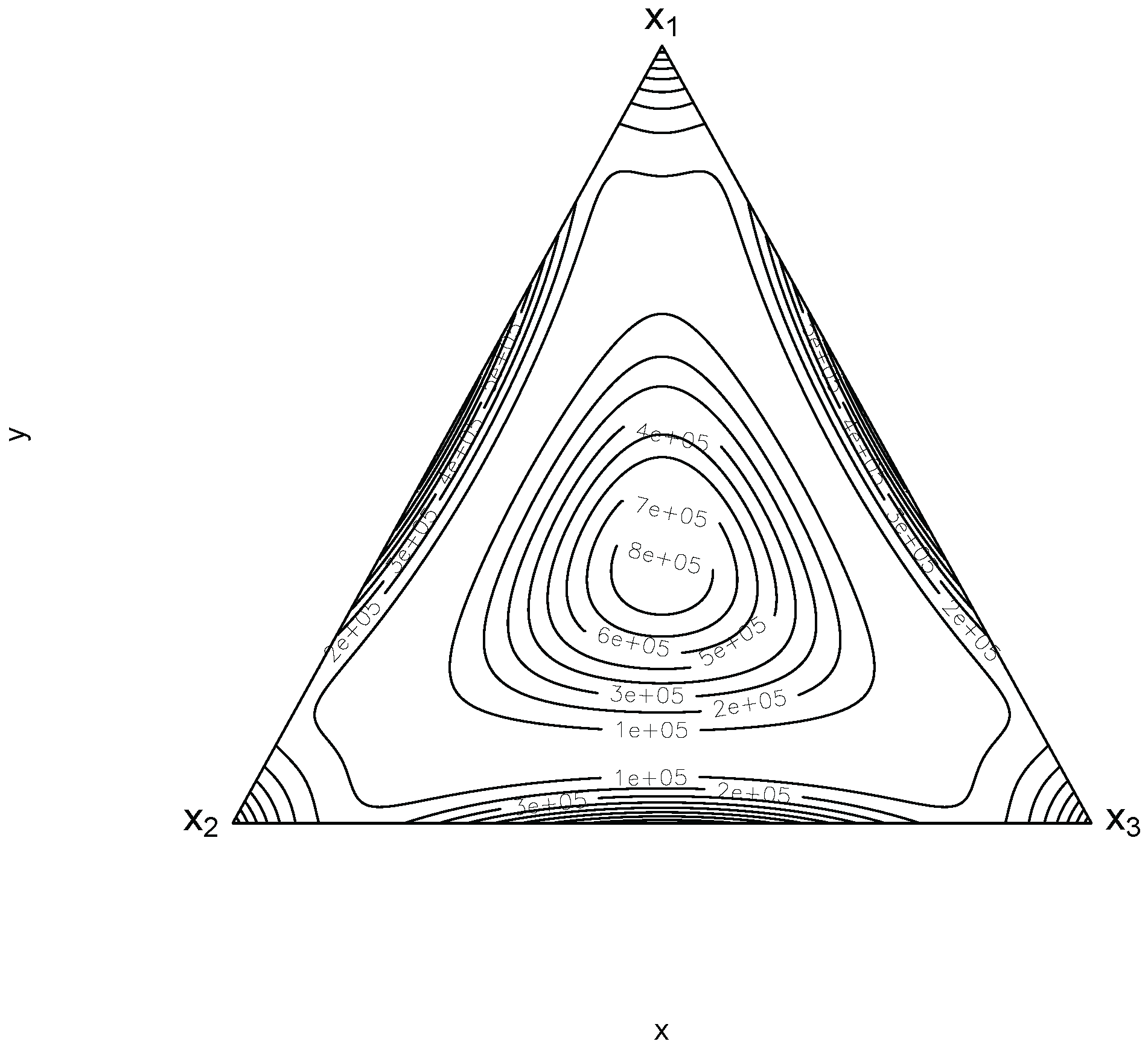
Figure 1. When x 4 = 0 is the variance function graph of A-optimal design for Model (7).
Preprints 113487 g001
Disclaimer/Publisher’s Note: The statements, opinions and data contained in all publications are solely those of the individual author(s) and contributor(s) and not of MDPI and/or the editor(s). MDPI and/or the editor(s) disclaim responsibility for any injury to people or property resulting from any ideas, methods, instructions or products referred to in the content.
Copyright: This open access article is published under a Creative Commons CC BY 4.0 license, which permit the free download, distribution, and reuse, provided that the author and preprint are cited in any reuse.
Prerpints.org logo

Preprints.org is a free preprint server supported by MDPI in Basel, Switzerland.

Subscribe

© 2024 MDPI (Basel, Switzerland) unless otherwise stated