Numerical Analysis of the Effect of Different Nose Shapes on Train Aerodynamic Performance

This study investigated the aerodynamic performances of various trains with different nose shapes, using as design variables two angles α,β for the heads shape and the bluntness angle γ, without crosswind. The effect on aerodynamic performances, such as the train drag coefficient, pressure distribution along the train surface, flow structures around the train and the wake, head pressure pulse, were analyzed. The results indicate that the increase of the train nose length for flat shapes decreases the CD values by 21.47% and 19.11%, decreasing the high-pressure region in the leading head. The duck-nose configuration emerges as a compromise between drag reduction and nose length. Increasing the angle γ a further drag reduction of 8.5% is featured. Drag formation along the train is also analyzed. The steeper the variation of the geometry, the higher the peak intensity and the slope of the curve. Regarding the flow features around the train, two-main counter-rotating vortices are captured in the wake. Moreover, the higher the nose length and the higher the bluntness angle γ, the weaker and narrower the wake. Again, a longer nose shape yields to a softer jump in terms of pressure difference, crucial for train homologation and safety.

Keywords:

Subject: Engineering - Aerospace Engineering

1. Introduction

High-speed trains have become increasingly significant in people’s lives with advancements in high-speed railway technology. Simultaneously, researchers are actively exploring the aerodynamic characteristics of these trains. Previous studies underscore the correlation between the shape of high-speed trains and their aerodynamic performance, highlighting the significance of factors such as bluntness, A-pillar roundness, and nose length (Niu et al. [1], Oh et al. [2], Munoz-Paniagua et al. [3]). Researchers have conducted parametric analyses to discern the governing parameters influencing aerodynamic drag. These investigations, employing numerical simulations and scaled models in wind tunnels, scrutinized variables like train speed, cross-sectional area, distance between passing trains and adjacent structures, ground clearance, and overall train and line geometry (Rocchi et al. [4], Meng et al. [5], Zampieri et al. [6]). The impact of train nose length emerged as a noteworthy aspect in these studies. Longer streamlined train heads were found to correlate with a reduction in total drag coefficient, diminished strength of wake flow, and the generation of a minor positive pressure area in the nose cone [7]. Baker [8] conducted an analysis of the airflow around high-speed trains in a zero crosswind condition, focusing on three distinct flow regions: the frontal area around the train’s front, the boundary layer along its length, and the wake region behind it. Moreover, in open air without crosswind, the slipstream produced by high-speed trains and operational freight trains [9] holds particular importance, particularly in the wake of high-speed trains (Osth et al. [10], Bell et al. [11]). When the train speed increases, the shape of the train directly affects its aerodynamic performance, which includes aerodynamic forces, slipstream and wake flow (Hemida et al. [12]). Previous research shows that the characteristics of train drag are significantly related to the shape of the train head and that the train nose length has a great effect on improving the train aerodynamic performance (Schetz [13], Raghunathan et al. [14]). Many experts and scholars have performed various optimization studies on the nose shape of trains to improve the aerodynamic performance of trains in open air and tunnels (Yang et al. [15], Yao et al. [16], Suzuki and Nakade [17], Li et al. [18]). To date, some scholars have studied the effect of the train nose length on the train aerodynamic performance. Choi and Kim [19] studied the effects of the train nose length on the aerodynamic drag of trains travelling in tunnels with the speed increasing from 100 to 200

k m / h

and found that the aerodynamic drag is reduced by up to approximately

50 %

by changing the nose from a blunt to a streamlined shape. Hemida and Krajnovic [20] investigated the influence of the nose shape on the train flow structures under a crosswind and found that the flow around the nose yielded more vortex structures in the wake in the short-nose simulation. Hemida and Krajnovic [21] found that the influence of different nose lengths on the surface pressure on the train body was mainly concentrated at the front and rear of the train. Chen et al. [22] compared and discussed the pressure distribution on the train surface, vortex development, and variation of the velocity field around the train. Chen et al. [23,24] studied the influence of the train nose length on the aerodynamic properties using the detached-eddy simulation (DES) method and found that the total drag coefficient, strength of vortex shedding, and strength of the wake flow decreased with increases in the train nose length and a minor positive pressure area was generated in the nose cone compared to a shorter train nose. Tian [25] analyzed the formation mechanism of aerodynamic drag of high-speed trains and found that adopting a streamlined train shape is the most effective measure to reduce the aerodynamic drag. Tian et al. [26] studied the influence of a streamlined head shape on the air pressure pulse and found that as the length of the streamlined train head increases the amplitude of the air pressure pulse decreases logarithmically while the absolute value of the aerodynamic drag of head-car decreases linearly and the aerodynamic drag of the tail-car decreases by quadratic.

The wind tunnel test is a widely used method for studying the aerodynamic performance of trains (Niu et al. [27], Kwon et al. [28]). The aerodynamic characteristics of different high-speed train models were compared by conducting wind tunnel tests with different slenderness ratios (Zhang and Zhou [29]). The results indicated that when the difference in streamline nose lengths of the model trains is not large, the larger slenderness ratios, i.e., the thinner and longer head car, are more favorable for the reducing drag. The overarching objective of this research is to scrutinize the flow field around high-speed trains, specifically focusing on various nose shapes, and discern their impact on aerodynamic drag. The paper is organized as follows: starting with the model of the train and the definition of the angles for the parametric analysis in Section 2, the numerical model, grid generation, computational domain and boundary conditions are presented in Section 3. After the mesh convergence study and the farfield indipendence analysis in Section 4, the results and the effect of the design variables on the aerodynamic performances and flow features are presented in Section 5. A summary and outlook is given in Section 6.

2. Train Model

The train geometry has been based on the Alstom AGV high-speed EMU for car dimensions and Jacob bogies configuration [30,31]. The CAD model has been realized using SolidWorks 2022. The AGV uses 11 coaches in the version ran by Italo-NTV, but it has been chosen to modelize only 3 coaches to optimize train length (to still have room for a standard coach in-between the extremities) and computation time. The train is symmetrical in both lateral and longitudinal direction, with both end cars sharing the same nose shape in all configuration studied. The modelized bogies also share the same CAD model based on the AGV Jacob bogie dimensions [30].

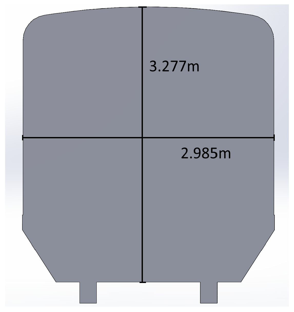
The train dimensions are as follows:

Table 1. Geometric description

Dimension	Value	SI Unit
Train Length	52.0	m
Leading Car	17.1	m
Middle Car	17.8	m
Car Height	3.277	m
Car Width	2.985	m
Frontal Area	9.773	$m^{2}$

Figure 1. Dimensions of the full-scale train

Figure 2. Train frontal area

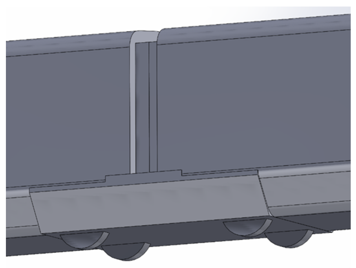
The objective of this study is to analyze the influence of the nose shape on high-speed train aerodynamic performances; therefore, the train geometry has been simplified to reduce interferences around bogies and cars separations, and no pantographs have been modeled. All the nose fillets used have been chosen with a

300 m m

radius to have a realistic geometry.

Figure 3. Train bogie and intercar

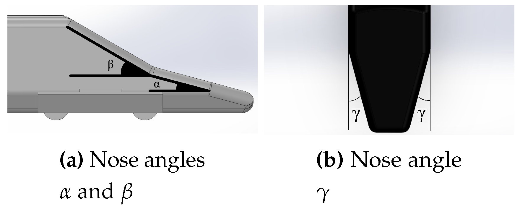
The parametrization of the nose consists of two angles

α

and

β

, with values changing between 15°, 30° and 50°, giving a total of nine combinations. It has also been chosen to set length of both nose parts to be equal (therefore nose length changes depending on the two angles). In the second part of the study is introduced on the train nose also the angle

γ

, with the objective to study the aerodynamic effect of an angle defined on another plane. This angle begins

3 m

after the nose, so that there is no influence from the bogie located just further back.

Figure 4. Train nose parametrization

3. Numerical Model

3.1. Numerical Setup

In this study, steady-state incompressible RANS simulations were performed, using the open source toolbox OpenFOAM. It employs the SIMPLE (Semi-Implicit Method for Pressure Linked Equations) algorithm to solve the continuity and momentum equations. The flow is initialized by means of potential equations, largely used to initialize the internal fields away from walls for viscous computations. Turbulence was modeled using

k - ω - S S T

due to its higher performance in operating with separated flows and with strong adverse pressure-gradients. Based on a uniform free-stream velocity of

60 m / s

aligned with the longitudinal axis, and the train height H, the Reynolds number is ≈

10^{7}

. Since the Mach number is approximately

0.175

, the airflow can be treated as an incompressible fluid for the solution. The Gauss scheme is used as discretisation scheme, adopting a second order scheme for the dissipative term, a first order scheme for the turbulence, and a first to second order scheme for the convective term, as interpolation schemes. Moreover, wall functions are used to avoid resolving the boundary layer, getting a significant reduction of the mesh size and computational cost, ensuring that the first grid cell is

30 < y^{+} < 300

Finally, the drag coefficient

C_{D}

is defined as follows:

C_{D} = \frac{D}{\frac{1}{2} ρ U_{\infty}^{2} S}

(1)

where D is the aerodynamic drag force,

ρ

the air density,

U_{\infty}

the free-stream velocity and S the body frontal area.

3.2. Grid Generation

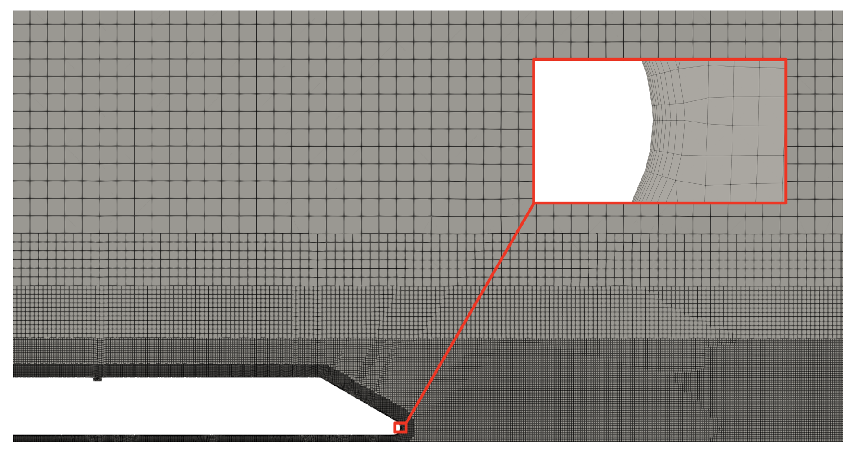
The grids of the models were generated using the

s n a p p y H e x M e s h

utility which was within OpenFOAM, which has been widely and successfully applied in aerodynamic numerical simulation of trains [32,33]. The meshes were dominated by hexahedral cells. To obtain more efficient use of computing resources, different refinement levels were applied to achieve a better transition of mesh density from domain surfaces to that of the train, as shown in Figure 5. Coarse, medium and fine refinement boxes corresponding to Level 1,2,3 respectively, and Level 4 up to

0.8 m

from the train surface are generated, in order to ensure that the size of the boundary layer gradually transitions to the size of the main grid. As can be seen in Figure 6, ten prism layers were attached on the train surfaces, where a thickness growth factor of 1.3 was used and the thickness of the layer furthest away from the wall is the

30 %

of the undistorted size of cell outside layer. These prism layers guaranteed a better capture of the near-wall flow structure.

3.3. Computational Domain and Boundary Conditions

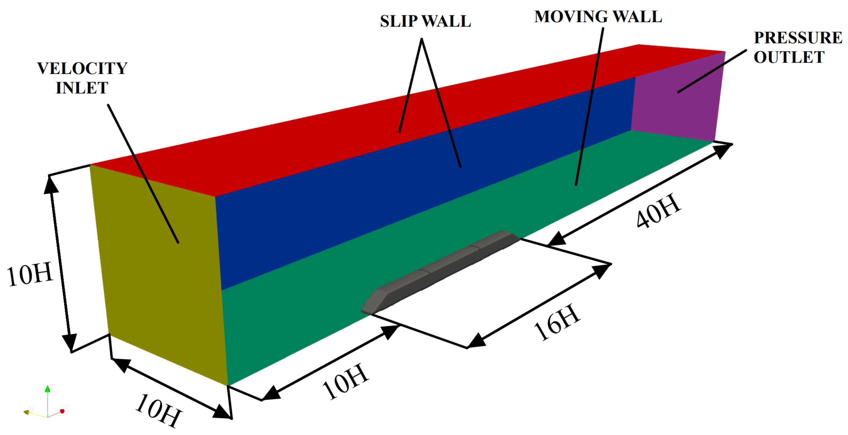
The computational domain used in this paper is shown in Figure 7. H is the train equivalent height. The boundary of the calculation domain should be as far away from the body as possible to eliminate the interference of the calculation domain boundary on the flow field around the train. However, the computing domain should not be excessively large to reduce the number of cells and improve the computing efficiency. The size of the domain comes from a farfield indipendence study, illustrated in Section 3. The distances from the head car nose to the upstream boundary and from the side boundary to the longitudinal center of the train body are 10 H. The inflow side is set as velocity inlet boundary condition. Considering the full development of the wake flow, the exit boundary is set as the zero-pressure outlet. The distance from the downstream boundary to the tail car nose point is 40 H. The height of the calculation domain is 10 H. In order to simulate the actual running state of the train, the train is stationary, the ground is set to moving wall boundary condition, the speed is given as the train speed, and the upper and the side surfaces are set to the slip wall boundary condition. As a consequence on the train body a no-slip boundary condition has been applied. As steady 3D CFD simulations were performed, on a semi-train endowed with a longitudinal plane of symmetry, only half of the actual fluid volume around the body was considered, in order to reduce time and resources required by each simulations, hence a symmetry boundary condition is set to the side that matches the longitudinal plane of symmetry of the train body.

4. Validation

4.1. Convergence and Mesh Indipendence Study

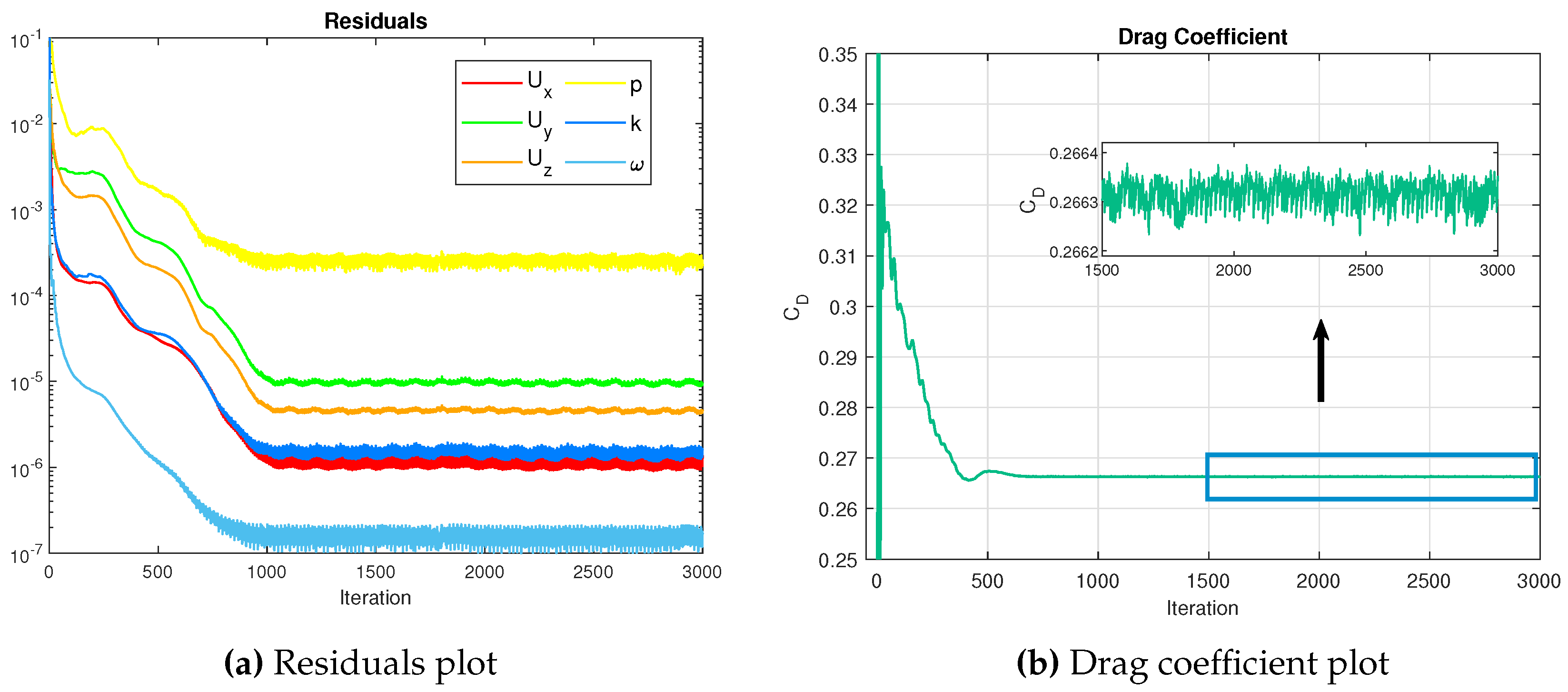
To check the convergence of a Steady State Simulation it is needed to ensure that the residual values of the conserved variables have been reduced to an acceptable value and that the main output of the simulation has reached a steady solution, namely the behaviour of the force coefficient started showing a periodicity or confined oscillations around a constant mean value.

The residuals in Figure 8a, representative of the percentage of the force imbalance, are computed using the

L^{1} - n o r m

inside the CFD solver. As can be seen in Figure 8b, all results presented later were obtained through averaging on a window among the last 1000 or 1500 iterations.

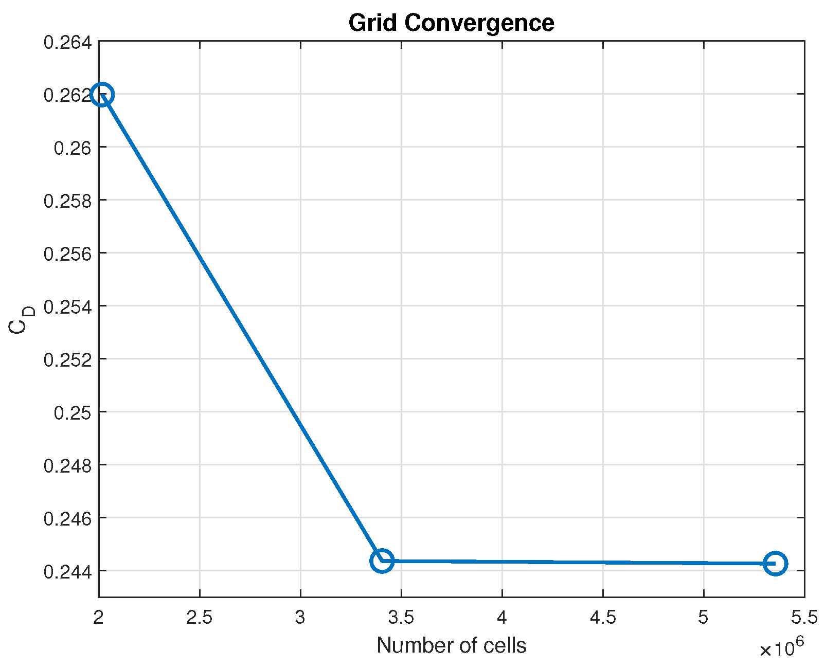
Grid refinement strongly affects the number of cells and, hence, the computational cost of the simulation. The number of elements was in fact limited by the available computational resources, to a maximum of

5 \div 6

millions of cells. The refinement is pursued by simply controlling the size of the furthest cell from the train surface (i.e. Level 0), keeping fixed the proportion between the boxes.

The results in Figure 9 and in Table 2 show a convergent behaviour, yielding to a variation of 0.04% between the last two grids, thus the second-last was picked, ensuring to save computational time without losing in accuracy.

4.2. Farfield Indipendence

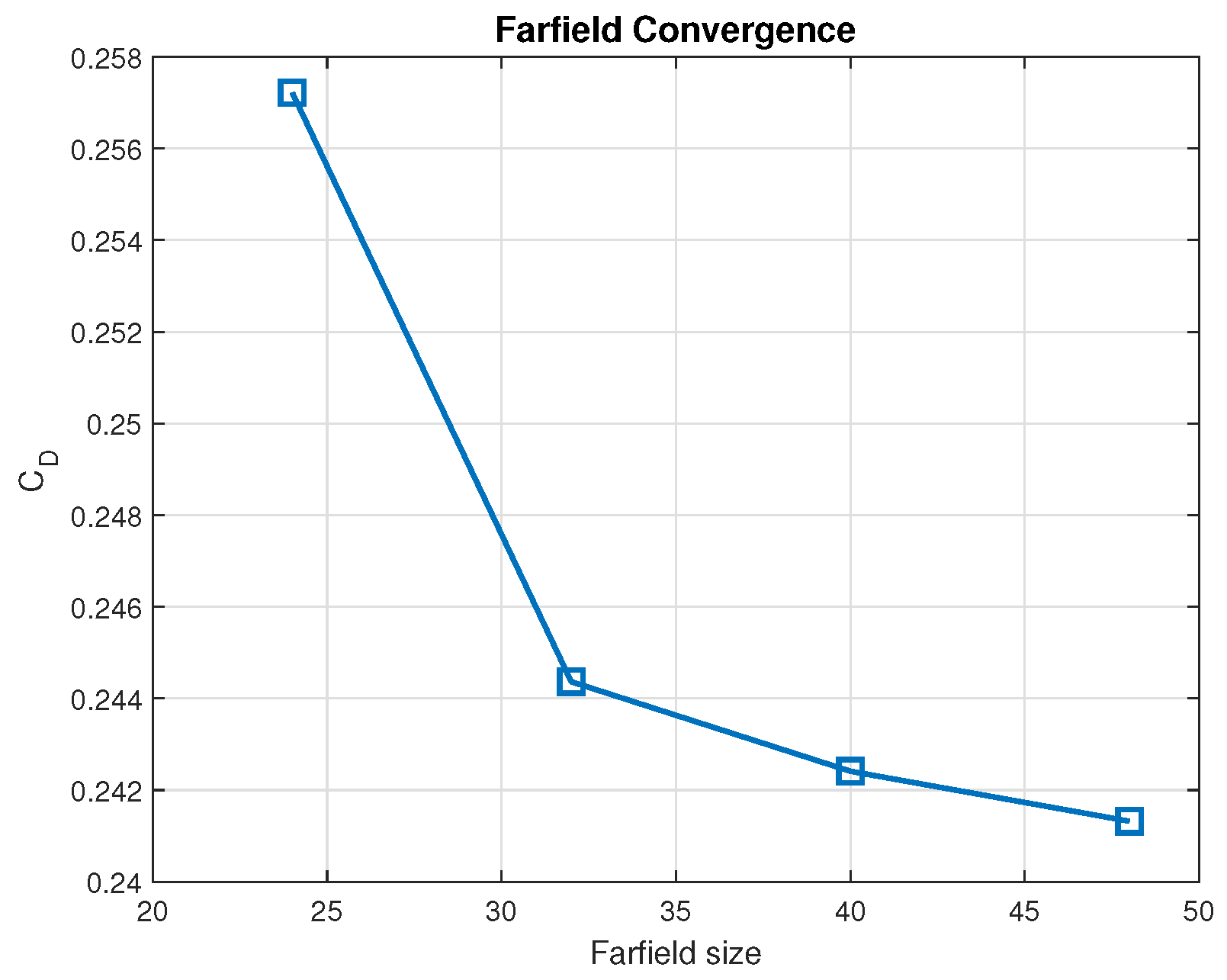
The purpose of the farfield indipendence study is to verify that the flow features do not depend on the size of the domain. The volume should be neither too small to avoid boundary effects, nor too large due to a useless memory storage.

The refinement boxes and the cells are kept constant in size in this analysis. Different domains are obtained by scaling downstream and upstream lengths of the same factor, and consequently get the dimensions towards up and right. Figure 10 shows that a farfield-indipendent solution is achieved, yielding a drag coefficient variation of less than 1%. All the following simulations are performed with the green-highlighted one in Table 3.

5. Results and Discussion

5.1. Effect of the Design Variables $α$ and $β$

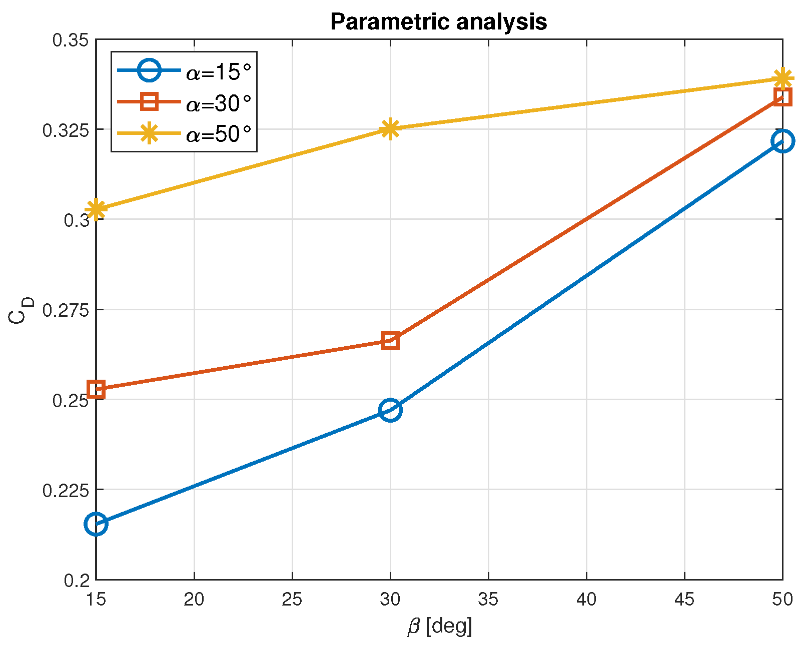
Figure 11 shows the results of different configurations of the train nose shape. For a flat geometry, the drag coefficient gets larger with the design variable

α

, thus the increase of the train nose length decreases the

C_{D}

values of the whole train by

21.47 %

and

19.11 %

. Furthermore, low values of

α

provide greater sensitivity to the second design variable

β

; on the other hand, for high values of

α

the drag coefficient curve tends to be flattened by reason of high values of

β

. Basically, high values of

α

do not lead to a

C_{D}

optimization, but for high values of

β

also low

α

train configurations can yield to very high drag coefficients. Finally, the lowest value of the drag coefficient is given by the largest train nose length, with a flat shape, providing a

C_{D} = 0.2154

while the second best value is given by the duck-nose shape (

α = 15^{\circ}, β = 30^{\circ}

), providing a

C_{D} = 0.2470

. It can be noticed that the curves are converging after

β = 30^{\circ}

, where the rise of

β

on the duck nose prevails in terms of boosting up the

C_{D}

value of the train, and the reason is that the upper wall of the nose tends to be more vertical, causing a very high pressure drag.

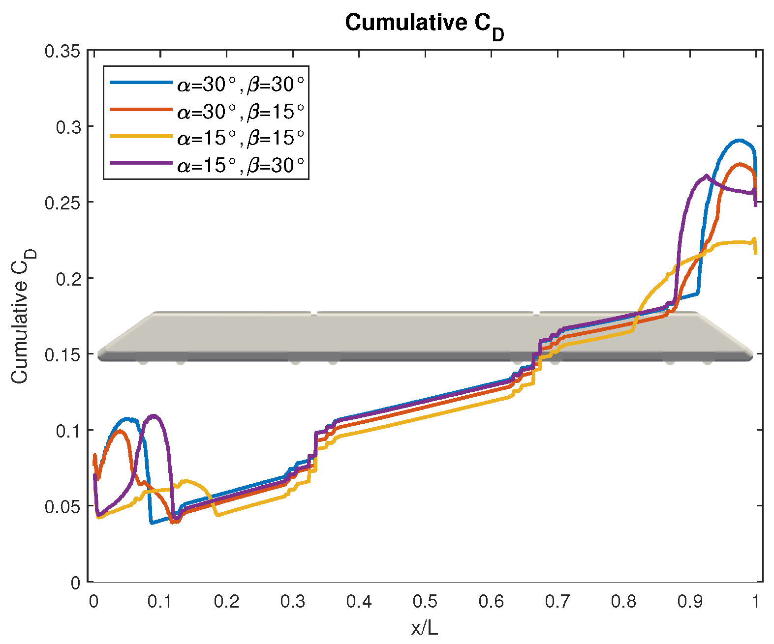
Figure 12 illustrates how the drag coefficient progresses along the train. The longer the head car nose, the lower the peak intensity and the slope of the curve. Similar behaviour can be expected from the combination of two angles, if the starting angle is large, the increase of the drag is faster, while if the starting angle is low, a significant generation of the drag occurs later. Then, there is a zone in which the flow is accelerating and the pressure decreases, resulting in a negative force, thus the train is pulled upstream and the cumulative drag drops.

Along the main train body, the drag increases slowly due to the friction forces and it features two small peaks due to the two inter-car gaps.

In the rear part of the train, when the flow encounters a large curvature of the tail, the increase of the drag is steeper than with a smoother variation of the geometry.

At the rear of the duck-nose configuration (purple curve), the flow encounters firstly an abrupt variation in the geometry, thus the curve features a steep increase of the drag, and secondly a positive pressure zone that pushes upstream the train, resulting in a drag reduction. Optimizing the aerodynamic shape for drag reduction mainly comes from reducing the pressure drag of the train, and pressure drag mainly exists on the front cone and the tail cone.

5.2. Pressure Distribution

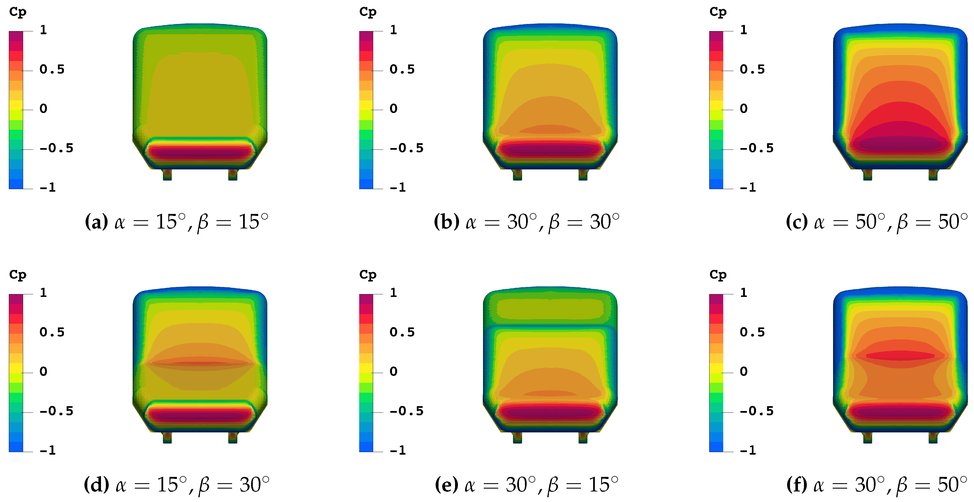
The drag difference is analysed from the perspective of the pressure distribution. The pressure distribution on the head coach surface is shown in Figure 13, in terms of pressure coefficient

C_{p}

, defined by:

C_{p} = \frac{p - p_{\infty}}{q_{\infty}}

(2)

where p is the local static pressure,

p_{\infty}

the free-stream static pressure and

q_{\infty}

the free-stream dynamic pressure. A large area of high-pressure exists at the stagnation point, giving a backward push to the nose cone of the train coach, increasing the pressure drag. Lower the train nose length, more negative the static pressure at the top, giving a higher reduction on the drag, but starting from an higher value of the cumulative drag. At the front of the optimal train, the high-pressure region is smaller than the corresponding high-pressure region of the other trains. The decrease in size of this high-pressure region reduces the drag. The train with a duck-nose configuration exhibits an additional high-pressure zone close to the windshield, leading to a heightened

C_{D}

compared to the ideal design.

Overall, the increase of the train nose length reduces the size of the high-pressure region in front, leading to a reduction of the drag.

While keeping fixed the first design variable

α

, it is always better to decrease the second design variable

β

, resulting in a reduction of the drag.

Comparing the trains in Figure 13e,d, with the same

α

and

β

values but switching the order, results in a lower drag for the configuration with a lower value of the first angle, namely the duck-nose shape. Similarly, the pressure distribution around the trailing cars yield to positive pressure areas that give a forward push, lowering the pressure drag. Higher the curvature of the geometry, namely lower the train nose length, higher the acceleration of the flow at the top, and lower the pressure, resulting in a faster increase of the drag.

5.3. Flow Field Analysis

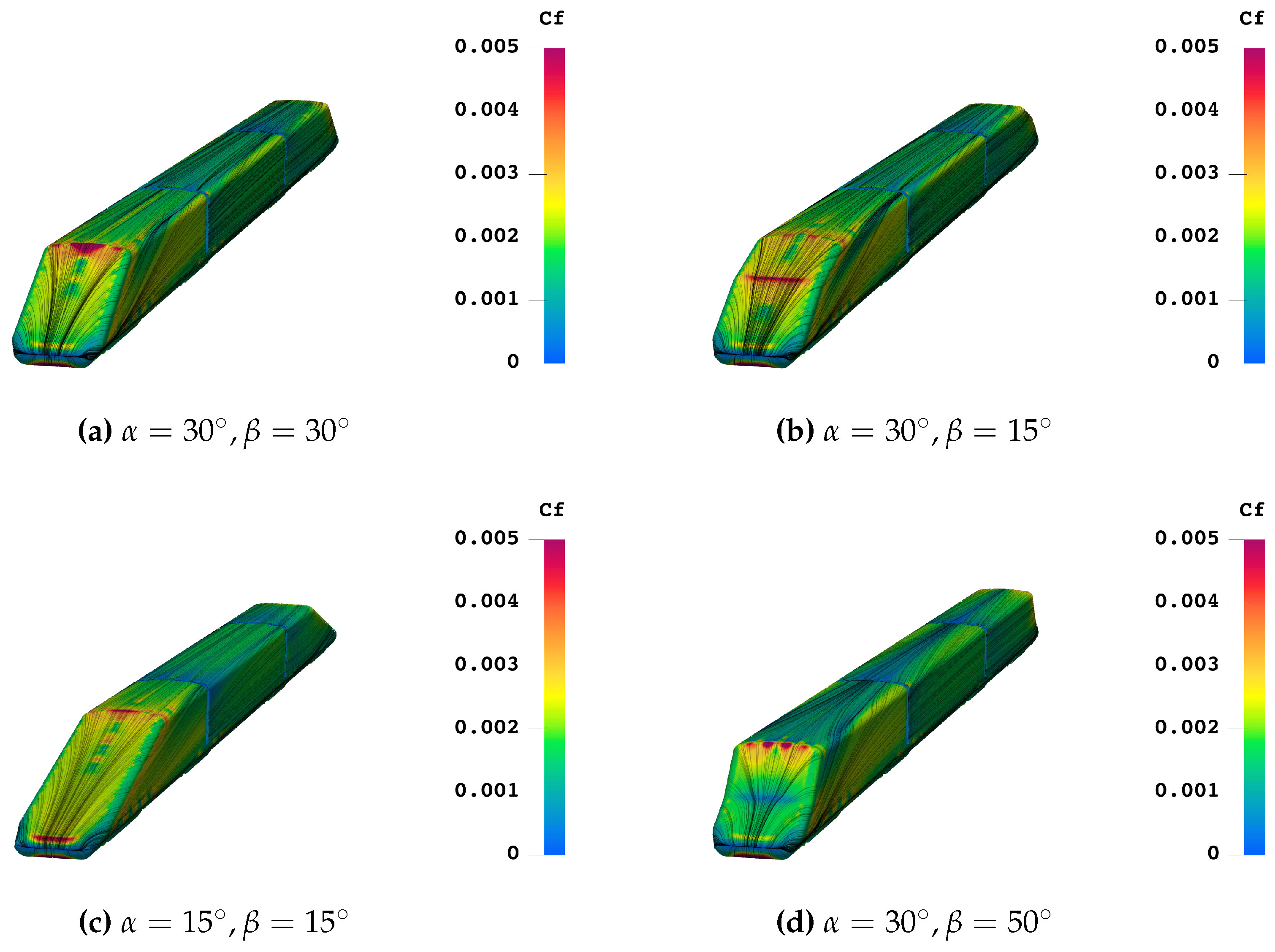
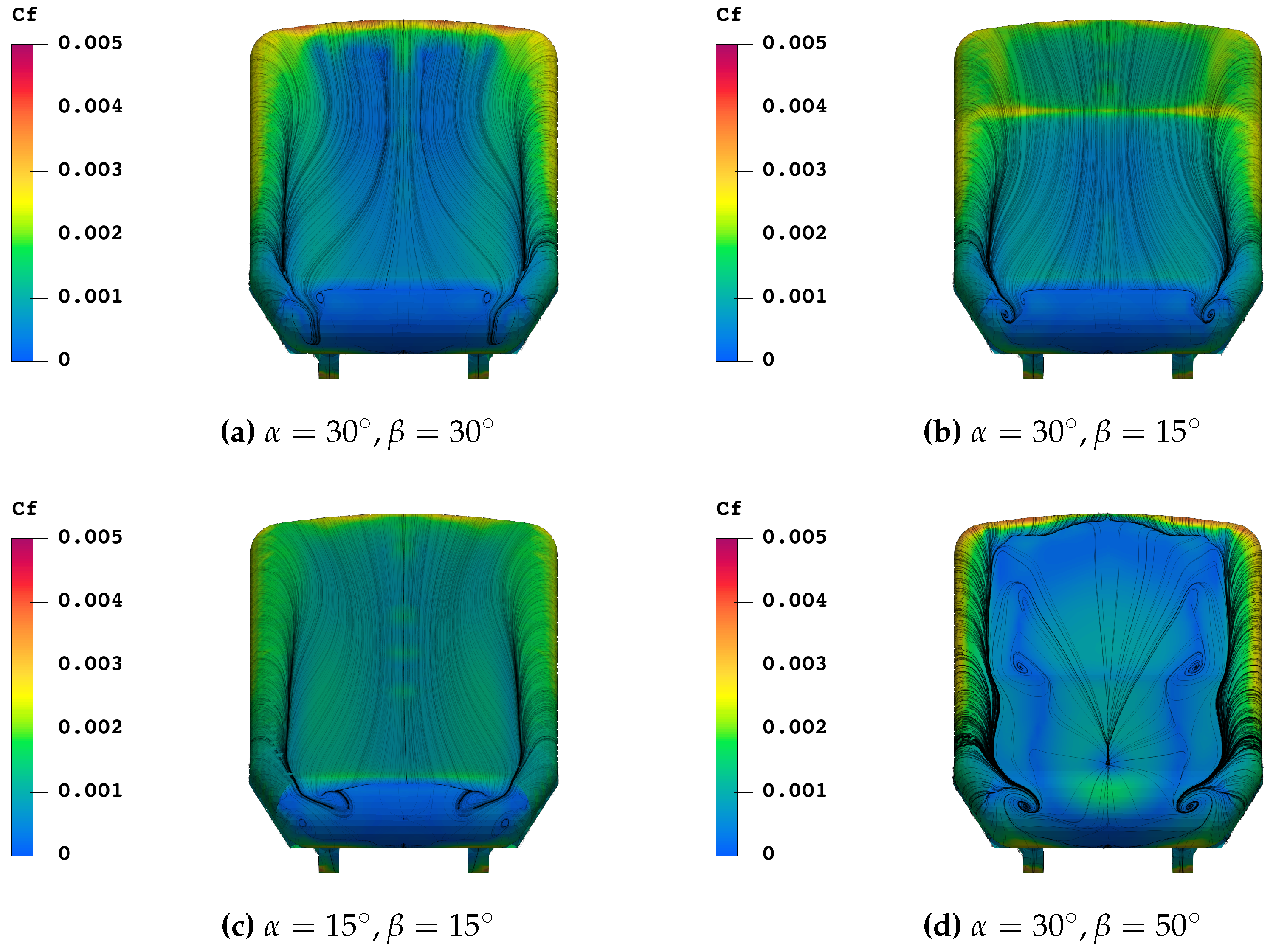
Figure 14 shows the limiting streamlines superposed on skin friction coefficient distribution on the train surface. The skin friction coefficient

C_{f}

is defined by:

C_{f} = \frac{τ_{w}}{q_{\infty}}

(3)

where

τ_{w}

is the local wall shear stress and

q_{\infty}

is the free-stream dynamic pressure.

Examining the level of surface friction, the green areas signify that the air is conforming to the contours of the train’s geometry, indicating a state of attached flow. At the stagnation point, the wall shear stress is lower. However, in the vicinity of the leading edges around the stagnation point, where there is an abrupt change in curvature, the skin friction coefficient tends to be higher, as does on the first part of the roof of the train. Close to the inter-car gaps the skin friction coefficient tends to be lower, due to the separation of the airflow. After that, the flow tends to reattach again. Skin friction magnitude tends to be lower in the rear part, indicated by the blue zones, which means that the flow is no more attached. It’s also clearly visible the attachment node on the stagnation point. Flow separation occurs at the top of the surface, where the separation line is generated from the fast convergence of the limiting streamlines coming from the side surface and the leading head. The higher the nose length, the lower the separation and consequently smaller longitudinal vortices are produced.

The limiting streamlines on the tail surface, as shown in Figure 15, are an aid to a better comprehension of the flow separation. The airflow separates when the limiting streamlines are converging rapidly, from which a separation surface is generated and goes into the flow field. In the duck-nose configuration, four foci and a saddle-point can be marked by the limiting streamlines, representing the generation of the vortex sheet, as shown in Figure 15d. As pointed out later on, as the train nose length increases, the wake becomes more narrowed, since the clearance between the two counter-rotating vortices is lower.

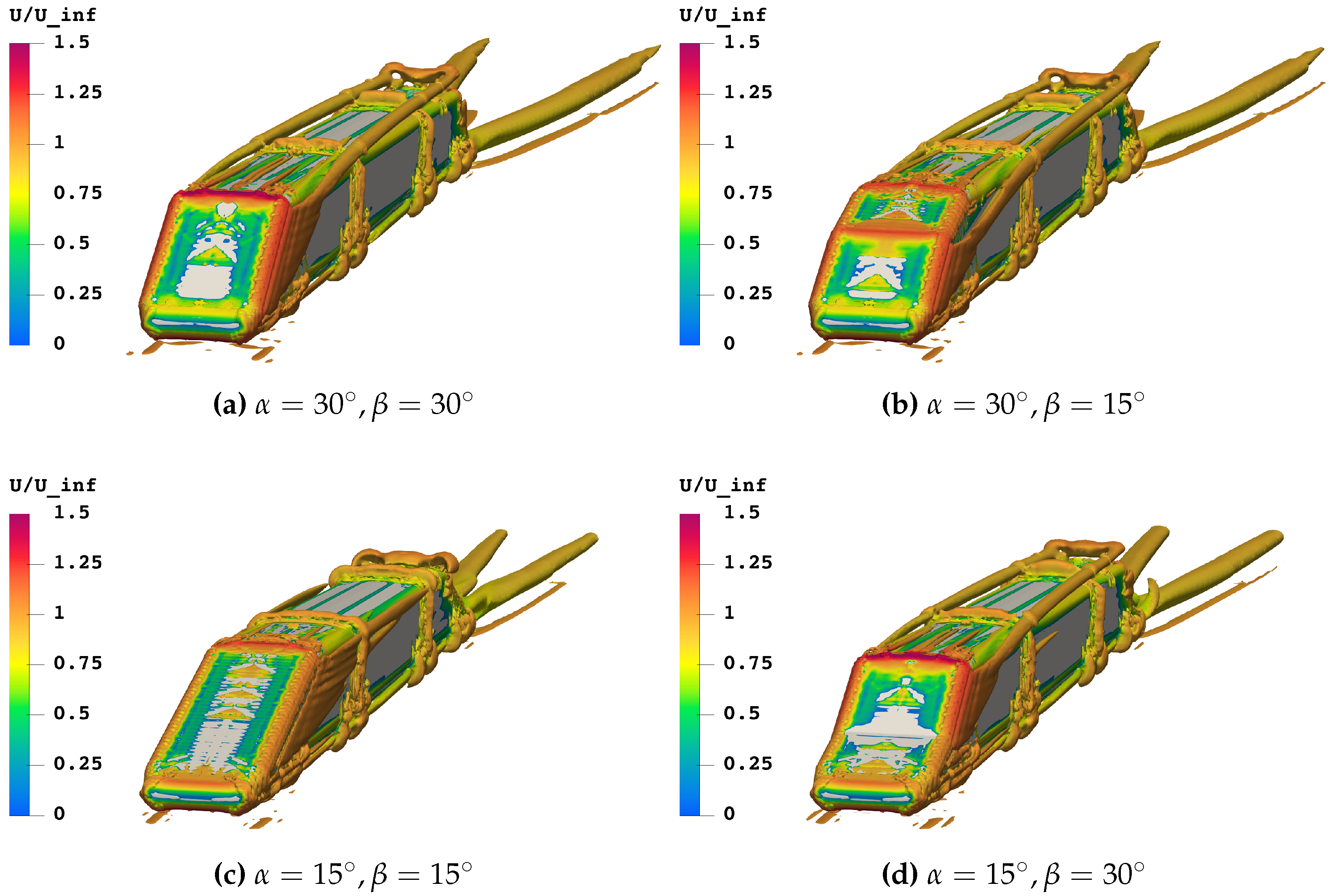
The vortex structure was described by the iso-surfaces of constant Q, which has been used for describing the flow structure around trains and has been used widely in studies of the aerodynamic performance of trains [20,34]. Figure 16 shows that the vortices around the train increase and strengthen from the train head to the train tail. Vortices around the train with a short train nose are bigger and stronger than those with a long train nose. Furthermore, in the latter one, the flow stays more attached to the train surface thus the separation is lower, and also the width of the wake is lower, yielding to a lower drag coefficient. Comparing Figure 16b and Figure 16d, the roll-up of the vortex sheet starts from the lower and from the higher A-pillar, respectively.

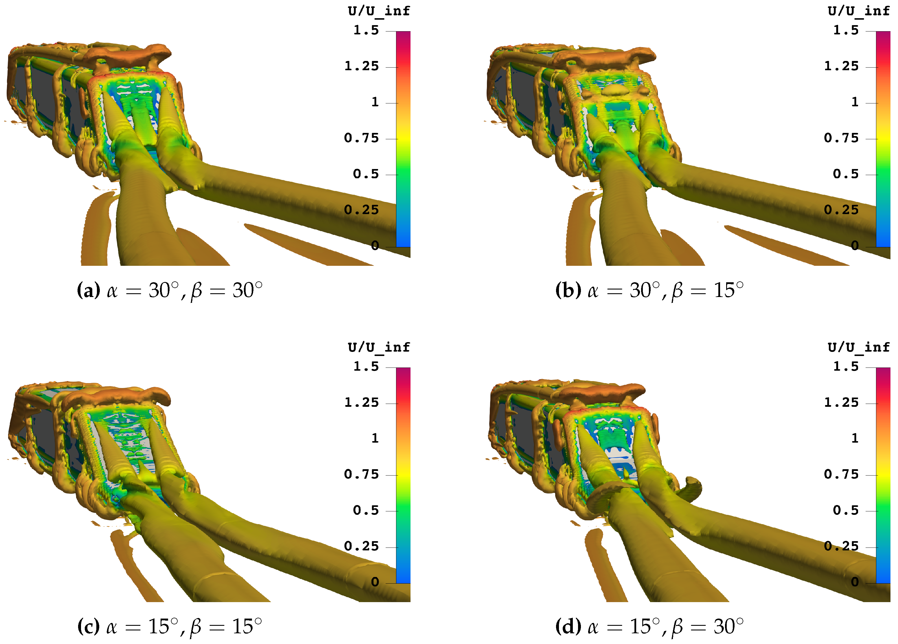
Figure 17 shows the vortex structure around the train tail. Longer the train nose, more slender is the wake. Organized longitudinal vortices are originated from the C-pillar on the train tail. In the configuration of

α = 15^{\circ}, β = 15^{\circ}

the flow remains attached on the inclined part, due to the induced velocity. For duck-nose configurations two couples of longitudinal vortices are expected to be generated from the rear part of the train (one weaker than the other) and it could be catched as the value of Q decreases, since the Q-criterion is sensitive to the isosurface threshold. If the threshold is too large, weak vortices will be wiped out. If the threshold is too small, weak vortices may be captured, but strong vortices could be smeared and become vague [35].

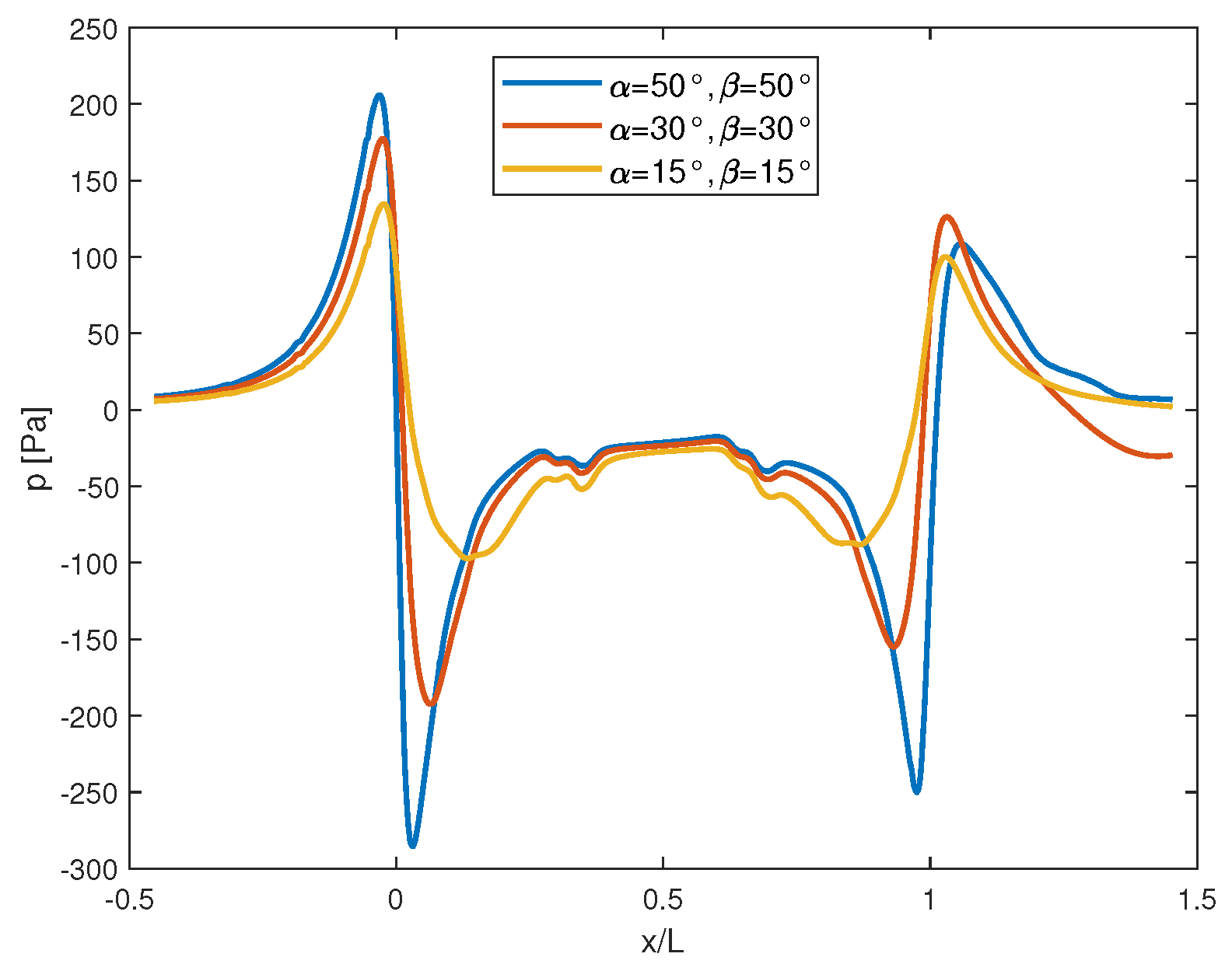
Figure 18 shows the pressure distribution along a line at a position 2.5 m sideways of the track’s centre line and at heights from 1.5 m above the ground. In the nose region a positive pressure occurs due to flow stagnation point and a negative pressure is caused by flow acceleration around the train nose shape. The greater the curvature imparted to the flow, the more negative the pressure and the steeper the variation. The pressure jump close to the train head with short nose (

α = 50^{\circ}, β = 50^{\circ}

) is larger than the configuration with long nose (

α = 15^{\circ}, β = 15^{\circ}

), stating that the separation of airflow is strongly affected by the shape of the train. Along the train body a slightly negative pressure region and pressure variations of lower magnitude due to inter-car gaps occur while in the rear part there is a negative to positive pressure transient, but smaller than the nose transient.

5.4. Effect of the Design Variable $γ$

In order to show a clear and better dependence from the bluntness variable, it has been decided to work on flat trains (

α

β

), keeping the focus on the aerodynamic effect of

γ

on the train without the coupled effect of

α

and

β

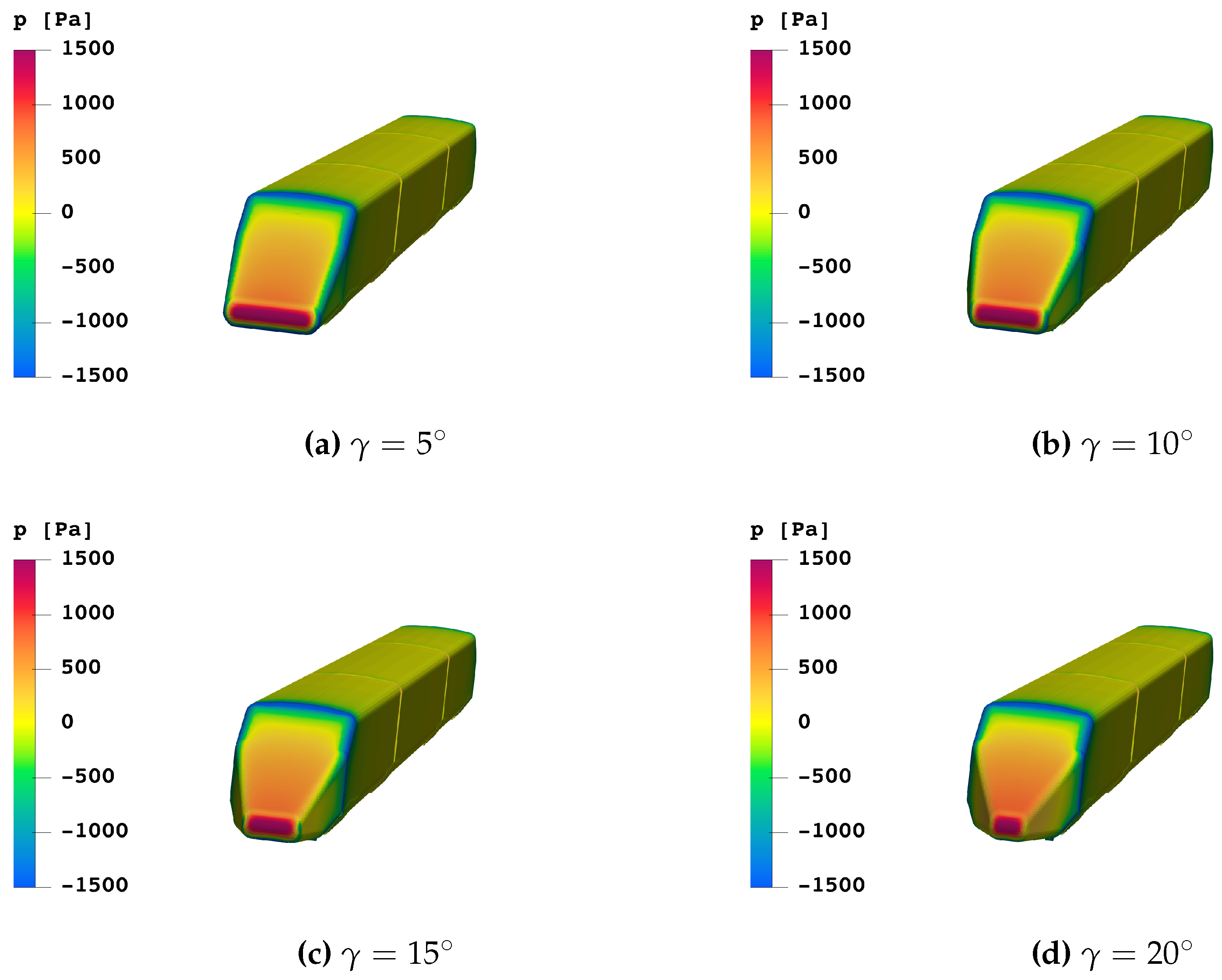
Figure 19 shows the drag coefficient of the trains with

α = 15^{\circ}, β = 15^{\circ}

and with

α = 30^{\circ}, β = 30^{\circ}

by varying the angle

γ

. The trend is that the higher the angle

γ

the lower the drag coefficient. It can be noticed that with short nose length, the slope of the curve is higher, thus the advantages of bluntness are more visible, while with long nose length the benefits are less marked, with a flatter trend. Finally, the train that features the lowest drag is with

α = 15^{\circ}, β = 15^{\circ}

and

γ = 20^{\circ}

, thus a long nose with pronounced sharpness, yielding to a value of

C_{D} = 0.1970

. However, it should be noticed that too long nose could cut out available space for passengers and utilities, thus the bluntness could be a good design variable in order to improve the aerodynamic performances of the high-speed train.

The pressure distribution at the train head surface is represented in Figure 20. Differences of the pressure distribution are observed at the nose tip, where a less blunt nose provokes a small area of high pressure, and so low aerodynamic drag. Thus a larger value of the design variable

γ

produces a lower drag coefficient, as the nose is sharper and more aerodynamic.

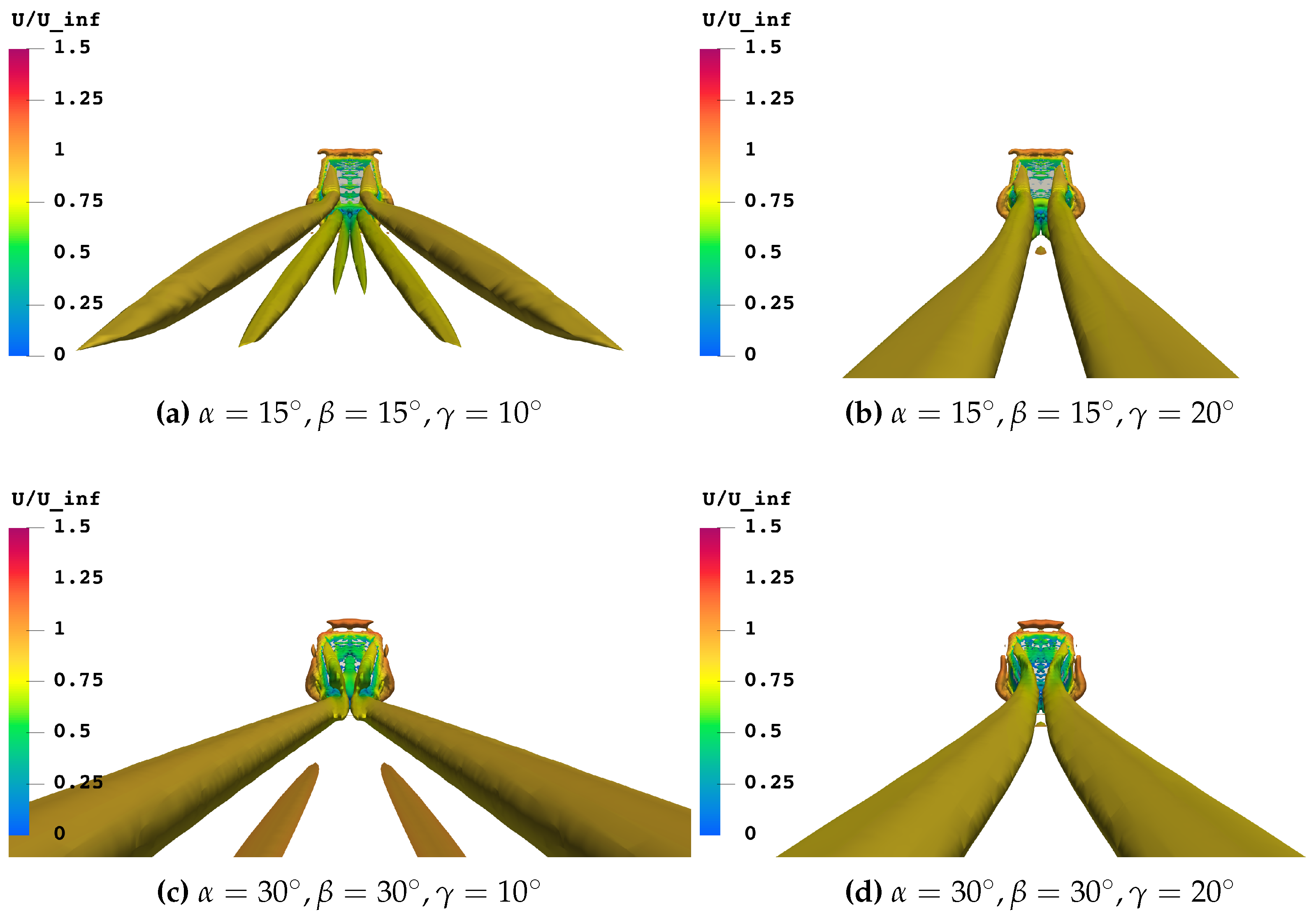
Figure 21 shows the rear vortices behaviour on

α = 15^{\circ}, β = 15^{\circ}

and

α = 30^{\circ}, β = 30^{\circ}

flat trains with a value of

γ = 10^{\circ}, 20^{\circ}

set on both configurations. Keeping fixed

γ

, passing from the

15^{\circ}

flat to the

30^{\circ}

, so by raising only

α

, there is an expansion in terms of vortex section that induces more drag, in addition to an increase in divergence of the longitudinal counter-rotating vortices. On the other hand, keeping fixed the nose slope, by increasing the angle

γ

the evolution is the opposite: the flow manages to detach from the train closer to the train longitudinal axis, resulting in a less wide wake.

6. Conclusions

The aerodynamic performance and flow fields for three-car trains with different nose shape were simulated without yaw angle. The conclusions drawn from the obtained results are as follows:

The parametric analysis of design variables $α$ and $β$ indicates that increasing both angle values leads to an elevation in the drag coefficient, $C_{D}$ . When $α$ is kept low, the drag coefficient experiences a more pronounced increase with a higher value of $β$ . Conversely, at high $α$ values, the growth of $C_{D}$ is more gradual with an increase in $β$ . Trains configured with $α = 50^{\circ}$ exhibit the highest $C_{D}$ values, primarily due to a notable surge in pressure drag on the nose, attributed to the pronounced inclination of the leading head. The low angles of $α$ and $β$ result in the minimum high-pressure region. Among the evaluated configurations, the train with the longest nose ( $α = β = 15^{\circ}$ ) achieves the lowest $C_{D}$ at 0.2154. Interestingly, a duck-nose configuration emerges as a favorable compromise between drag reduction and nose length. For $α = 15^{\circ}$ and $β$ ranging from $15^{\circ}$ to $30^{\circ}$ , this configuration features a $35 %$ shorter nose while experiencing a $14.67 %$ increase in $C_{D}$ .
From the flow field analysis, for streamlined shape body, a couple of counter-rotating vortices are generated from the train surface. Limiting streamlines coupled with iso-surfaces of Q-criterion are a good tool in order to understand the flow features around the train. The higher the nose length, the weaker and smaller the wake. For what concerns the pressure pulse, a longer nose produces a softer jump in terms of pressure difference. On the contrary the steeper the head, the higher the pressure pulse, constraining factor in terms of surrounding infrastructures and train crossing.
Examining the impact of the angle $γ$ from the analysis, results reveal that an elevation in the angle proves advantageous in the context of drag reduction. This is attributed to the minimization of the head high pressure region and the generation of vortices resulting in a narrower wake. Considering the optimal nose configuration identified in the prior analysis, an angle $γ = 20^{\circ}$ leads to a further drag reduction of $8.5 %$ , culminating in the most favourable $C_{D}$ value of the study, which stands at 0.1970.

Funding

“This research received no external funding”

Conflicts of Interest

“The authors declare no conflicts of interest.”

References

Niu, J.; Wang, Y.; Zhang, L.; Yuan, Y. Numerical analysis of aerodynamic characteristics of high-speed train with different train nose lengths. International Journal of Heat and Mass Transfer 2018, 127, 188–199. [Google Scholar] [CrossRef]
Oh, S.; Jiang, C.H.; Jiang, C.; Marcus, P.S. Finding the optimal shape of the leading-and-trailing car of a high-speed train using design-by-morphing. Computational Mechanics 2018, 62, 23–45. [Google Scholar] [CrossRef]
Munoz-Paniagua, J.; García, J.; Crespo, A. Genetically aerodynamic optimization of the nose shape of a high-speed train entering a tunnel. Journal of wind engineering and industrial aerodynamics 2014, 130, 48–61. [Google Scholar] [CrossRef]
Rocchi, D.; Tomasini, G.; Schito, P.; Somaschini, C. Wind effects induced by high speed train pass-by in open air. Journal of Wind Engineering and Industrial Aerodynamics 2018, 173, 279–288. [Google Scholar] [CrossRef]
Meng, S.; Li, X.; Chen, G.; Zhou, D.; Chen, Z.; Krajnovic, S. Numerical simulation of slipstreams and wake flows of trains with different nose lengths passing through a tunnel. Tunnelling and Underground Space Technology 2021, 108, 103701. [Google Scholar] [CrossRef]
Zampieri, A.; Rocchi, D.; Schito, P.; Somaschini, C. Numerical-experimental analysis of the slipstream produced by a high speed train. Journal of Wind Engineering and Industrial Aerodynamics 2020, 196, 104022. [Google Scholar] [CrossRef]
Xu, G.; Liang, X.; Yao, S.; Chen, D.; Li, Z. Multi-objective aerodynamic optimization of the streamlined shape of high-speed trains based on the Kriging model. PloS one 2017, 12, e0170803. [Google Scholar] [CrossRef] [PubMed]
Baker, C. The flow around high speed trains. Journal of Wind Engineering and Industrial Aerodynamics 2010, 98, 277–298. [Google Scholar] [CrossRef]
Flynn, D.; Hemida, H.; Soper, D.; Baker, C. Detached-eddy simulation of the slipstream of an operational freight train. Journal of Wind Engineering and Industrial Aerodynamics 2014, 132, 1–12. [Google Scholar] [CrossRef]
Östh, J.; Kaiser, E.; Krajnović, S.; Noack, B.R. Cluster-based reduced-order modelling of the flow in the wake of a high speed train. Journal of Wind Engineering and Industrial Aerodynamics 2015, 145, 327–338. [Google Scholar] [CrossRef]
Bell, J.R.; Burton, D.; Thompson, M.C.; Herbst, A.H.; Sheridan, J. Moving model analysis of the slipstream and wake of a high-speed train. Journal of Wind Engineering and Industrial Aerodynamics 2015, 136, 127–137. [Google Scholar] [CrossRef]
Hemida, H.; Baker, C.; Gao, G. The calculation of train slipstreams using large-eddy simulation. Proceedings of the Institution of Mechanical Engineers, Part F: Journal of Rail and Rapid Transit 2014, 228, 25–36. [Google Scholar] [CrossRef]
Schetz, J.A. Aerodynamics of high-speed trains. Annual Review of fluid mechanics 2001, 33, 371–414. [Google Scholar] [CrossRef]
Raghunathan, R.S.; Kim, H.D.; Setoguchi, T. Aerodynamics of high-speed railway train. Progress in Aerospace sciences 2002, 38, 469–514. [Google Scholar] [CrossRef]
Yang, X.; Jin, J.; Shi, G. Preliminary study on streamlined design of longitudinal profile of high-speed train head shape. Procedia-Social and Behavioral Sciences 2013, 96, 1469–1476. [Google Scholar] [CrossRef]
Yao, S.; Guo, D.; Sun, Z.; Yang, G. A modified multi-objective sorting particle swarm optimization and its application to the design of the nose shape of a high-speed train. Engineering Applications of Computational Fluid Mechanics 2015, 9, 513–527. [Google Scholar] [CrossRef]
Suzuki, M.; Nakade, K. Multi-objective design optimization of high-speed train nose. Journal of Mechanical Systems for Transportation and Logistics 2013, 6, 54–64. [Google Scholar] [CrossRef]
Li, R.; Xu, P.; Peng, Y.; Ji, P. Multi-objective optimization of a high-speed train head based on the FFD method. Journal of Wind Engineering and Industrial Aerodynamics 2016, 152, 41–49. [Google Scholar] [CrossRef]
Choi, J.K.; Kim, K.H. Effects of nose shape and tunnel cross-sectional area on aerodynamic drag of train traveling in tunnels. Tunnelling and Underground Space Technology 2014, 41, 62–73. [Google Scholar] [CrossRef]
Hemida, H.; Krajnović, S. LES study of the influence of a train-nose shape on the flow structures under cross-wind conditions 2008.
Hemida, H.; Krajnović, S. LES study of the influence of the nose shape and yaw angles on flow structures around trains. Journal of Wind Engineering and Industrial Aerodynamics 2010, 98, 34–46. [Google Scholar] [CrossRef]
Chen, X.D.; Liu, T.H.; Zhou, X.S.; Li, W.h.; Xie, T.Z.; Chen, Z.W. Analysis of the aerodynamic effects of different nose lengths on two trains intersecting in a tunnel at 350 km/h. Tunnelling and Underground Space Technology 2017, 66, 77–90. [Google Scholar] [CrossRef]
Chen, Z.; Liu, T.; Jiang, Z.; Guo, Z.; Zhang, J. Comparative analysis of the effect of different nose lengths on train aerodynamic performance under crosswind. Journal of Fluids and Structures 2018, 78, 69–85. [Google Scholar] [CrossRef]
Chen, Z.; Liu, T.; Zhou, X.; Su, X. Aerodynamic analysis of trains with different streamlined lengths of heads. 2016 IEEE international conference on Intelligent Rail Transportation (ICIRT). IEEE, 2016, pp. 382–387.
Tian, H.q. Formation mechanism of aerodynamic drag of high-speed train and some reduction measures. Journal of Central South University of Technology 2009, 16, 166–171. [Google Scholar] [CrossRef]
Tian, H.; Zhou, D.; Xu, P. Aerodynamic performance and streamlined head shape of train. China Railway Science 2006, 27, 47–55. [Google Scholar]
Niu, J.; Liang, X.; Zhou, D. Experimental study on the effect of Reynolds number on aerodynamic performance of high-speed train with and without yaw angle. Journal of Wind Engineering and Industrial Aerodynamics 2016, 157, 36–46. [Google Scholar] [CrossRef]
Kwon, H.b.; Park, Y.W.; Lee, D.h.; Kim, M.S. Wind tunnel experiments on Korean high-speed trains using various ground simulation techniques. Journal of Wind Engineering and Industrial Aerodynamics 2001, 89, 1179–1195. [Google Scholar] [CrossRef]
Dan, Z. Wind tunnel experiment on aerodynamic characteristic of streamline head of high speed train with different head shapes. 2013.
HUGHES, M. AGV tailors capacity and performance to the market. Railway Gazette International 2007.
Wang, J.; Minelli, G.; Dong, T.; He, K.; Gao, G.; Krajnović, S. An IDDES investigation of Jacobs bogie effects on the slipstream and wake flow of a high-speed train. Journal of Wind Engineering and Industrial Aerodynamics 2020, 202, 104233. [Google Scholar] [CrossRef]
Huang, S.; Hemida, H.; Yang, M. Numerical calculation of the slipstream generated by a CRH2 high-speed train. Proceedings of the Institution of Mechanical Engineers, Part F: Journal of Rail and Rapid Transit 2016, 230, 103–116. [Google Scholar] [CrossRef]
Morden, J.A.; Hemida, H.; Baker, C.J. Comparison of RANS and detached eddy simulation results to wind-tunnel data for the surface pressures upon a class 43 high-speed train. Journal of Fluids Engineering 2015, 137, 041108. [Google Scholar] [CrossRef]
Jeong, J.; Hussain, F. On the identification of a vortex. Journal of fluid mechanics 1995, 285, 69–94. [Google Scholar] [CrossRef]
Liu, C.; Gao, Y.s.; Dong, X.r.; Wang, Y.q.; Liu, J.m.; Zhang, Y.n.; Cai, X.s.; Gui, N. Third generation of vortex identification methods: Omega and Liutex/Rortex based systems. Journal of Hydrodynamics 2019, 31, 205–223. [Google Scholar] [CrossRef]

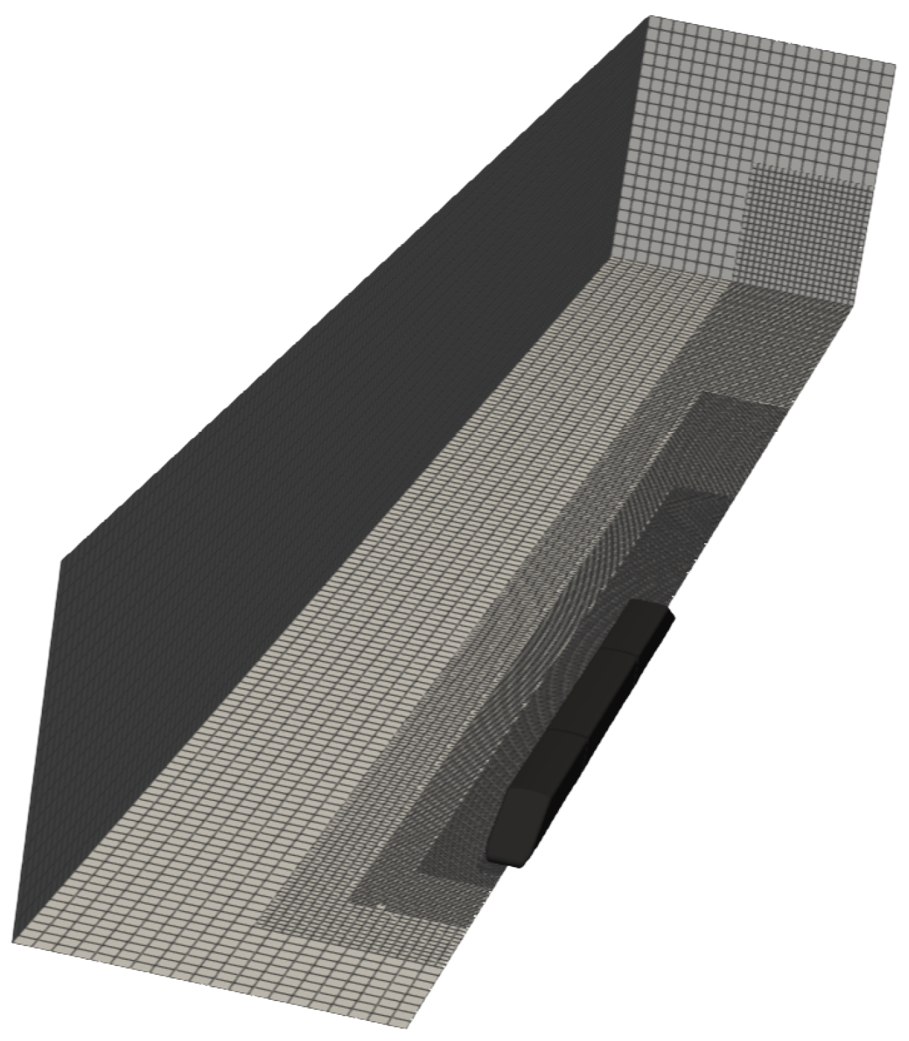
Figure 5. Computational domain and refinement boxes

Figure 6. Grid around the train

Figure 7. Computational domain

Figure 8. Convergence analysis

Figure 9. Mesh convergence, Drag coefficient

Figure 10. Farfield Convergence, Drag coefficient

Figure 11. Parametric analysis

Figure 12. Cumulative Drag Coefficient plot

Figure 13. Pressure distribution on leading heads

Figure 14. Limiting streamlines superposed on skin friction coefficient distribution on the train surface

Figure 15. Limiting streamlines superposed on skin friction coefficient distribution on the tail surface of the train

Figure 16. Iso-surfaces corresponding to the Q-criterion, rendered for dimensionless velocity magnitude (

Q = 10)

: vortex structure around entire train

Figure 16. Iso-surfaces corresponding to the Q-criterion, rendered for dimensionless velocity magnitude (

Q = 10)

: vortex structure around entire train

Figure 17. Iso-surfaces corresponding to the Q-criterion, rendered for dimensionless velocity magnitude (

Q = 10)

: vortex structure around train tail

Figure 17. Iso-surfaces corresponding to the Q-criterion, rendered for dimensionless velocity magnitude (

Q = 10)

: vortex structure around train tail

Figure 18. Pressure distribution along a line at one side of the train

Figure 19. Drag coefficient with different bluntness

Figure 20. Pressure field at the train head surface,

α = 30^{\circ}, β = 30^{\circ}

Figure 20. Pressure field at the train head surface,

α = 30^{\circ}, β = 30^{\circ}

Figure 21. Iso-surfaces corresponding to the Q-criterion, rendered for dimensionless velocity magnitude (

Q = 25)

: vortex structure around train tail

Figure 21. Iso-surfaces corresponding to the Q-criterion, rendered for dimensionless velocity magnitude (

Q = 25)

: vortex structure around train tail

Table 2. Grid Indipendence

Number of cells	$C_{D}$	$Δ C_{D} [%]$
2.0 x e6	0.2620	6.72
3.4 x e6	0.2444	0.04
5.4 x e6	0.2443	-

Table 3. Domain Indipendence

Domain [m]	$C_{D}$	$Δ C_{D} [%]$
150x18x18	0.2572	4.98
180x24x24	0.2444	0.82
216x30x30	0.2424	0.45
248x36x36	0.2413	-

Disclaimer/Publisher’s Note: The statements, opinions and data contained in all publications are solely those of the individual author(s) and contributor(s) and not of MDPI and/or the editor(s). MDPI and/or the editor(s) disclaim responsibility for any injury to people or property resulting from any ideas, methods, instructions or products referred to in the content.

© 2024 by the authors. Licensee MDPI, Basel, Switzerland. This article is an open access article distributed under the terms and conditions of the Creative Commons Attribution (CC BY) license (http://creativecommons.org/licenses/by/4.0/).

Copyright: This open access article is published under a Creative Commons CC BY 4.0 license, which permit the free download, distribution, and reuse, provided that the author and preprint are cited in any reuse.

MDPI Initiatives

Important Links

Choose an area of interest and we will send you notifications of new preprints at your preferred frequency.

Disclaimer

Numerical Analysis of the Effect of Different Nose Shapes on Train Aerodynamic Performance

Abstract

1. Introduction

2. Train Model

3. Numerical Model

3.1. Numerical Setup

3.2. Grid Generation

3.3. Computational Domain and Boundary Conditions

4. Validation

4.1. Convergence and Mesh Indipendence Study

4.2. Farfield Indipendence

5. Results and Discussion

5.1. Effect of the Design Variables α and β

5.2. Pressure Distribution

5.3. Flow Field Analysis

5.4. Effect of the Design Variable γ

6. Conclusions

Funding

Conflicts of Interest

References

MDPI Initiatives

Important Links

Subscribe

5.1. Effect of the Design Variables $α$ and $β$

5.4. Effect of the Design Variable $γ$