Preprint
Review

Study of Contactless Computer Vision-based Road Condition Estimation Methods within the Framework of an Operational Design Domain Monitoring System

Altmetrics

Downloads

136

Views

112

Comments

0

A peer-reviewed article of this preprint also exists.

This version is not peer-reviewed

Submitted:

30 July 2024

Posted:

01 August 2024

You are already at the latest version

Alerts
Abstract
Deployment of Level 3 and Level 4 autonomous vehicles (AVs) in urban environments is significantly constrained by adverse weather conditions, limiting their operation to clear weather due to safety concerns. Ensuring that AVs remain within their designated Operational Design Domain (ODD) is a formidable challenge, making boundary monitoring strategies essential for safe navigation. This study explores the critical role of an ODD monitoring system (OMS) in addressing these challenges. It reviews various methodologies for designing an OMS and presents a comprehensive visualization framework incorporating trigger points for ODD exits. These trigger points serve as essential references for effective OMS design. The study also delves into a specific use case concerning ODD exits: the reduction in road friction due to adverse weather conditions. It emphasizes the importance of contactless computer vision-based methods for road condition estimation (RCE), particularly using vision sensors such as cameras. The study details a timeline of methods involving classical machine learning and deep learning feature extraction techniques, identifying contemporary challenges such as class imbalance, lack of comprehensive datasets, annotation methods, and the scarcity of generalization techniques. Furthermore, it provides a factual comparison of two state-of-the-art RCE datasets. In essence, the study aims to address and explore ODD exits due to weather-induced road conditions, decoding the practical solutions and directions for future research in the realm of AVs.
Keywords: 
Subject: Engineering  -   Automotive Engineering

1. Introduction

In the quest to replace human drivers with machines and increase the level of autonomy in automobiles, researchers have made significant strides. Autonomous Vehicles (AVs) are no longer a distant possibility but an immediate reality and are the future of urban mobility. [1] divides the level of autonomy into six categories, where from L3 and above, the human driver is replaced by a computer with varying degrees of safety mechanisms. Designing and developing AVs at L3 and L4 autonomy has become more realistic and feasible from a technical viewpoint, but their deployment on the urban streets remains arduous and presents a completely different set of challenges. An AV must be proven safe before it is allowed to operate on public roads [2]. However, there has been a lack of consensus on defining safety.
The most common attempt to define safety has been to prove an absence of unreasonable risk [3]. Demonstrating that AVs are safer than a human driver (Positive Risk Balance) is one of the few approaches aimed at facilitating their deployment on urban streets without much hindrances, but has been deemed insufficient by various critics. Due to the lack of sufficient statistical data on AV mishaps, establishing a meaningful comparison is not possible. Simulating real-world edge cases is one way to generate statistics, but as there could be an unlimited number of such edge cases, some situations will inevitably be left untested. Nevertheless, various standards have been created to assist developers in ensuring safety, with some being very specific to AVs.
Several standards assist in ensuring the safety of automobiles in general, such as ISO 26262 [4], which focuses on the hardware part and lists tolerance and redundancy methods to overcome failures. ASPICE addresses the process followed during development, while ISO 21434 focuses on cybersecurity [5,6]. ISO 21448, known as the Safety of the Intended Functionality (SOTIF) [7], addresses the faults and failures, or Functional Insufficiencies (FIs), that could occur in the algorithms specific to AVs and the hazards that could arise from them. The functioning of these algorithms is highly scenario-based, and since it is impossible to predict how these algorithms will perform in every conceivable scenario, the testing strategy has to differ, and that is the idea behind SOTIF. To tolerate the FIs, SOTIF recommends certain test strategies and redundancy methods. However, SOTIF refrains from providing guidance on hazards that arise when an AV exits its intended operational boundary during real-time operation.
SAE levels L3 and L4 restrict the functioning of AVs within a defined operational region using an Operational Design Domain (ODD). An ODD outlines the specifications and conditions for which an AV is designed [1]. It provides a means to generate informed safety for the AV through the easy exchange of its capabilities and limitations among different stakeholders, thus restricting the area in which the AV can safely operate [8]. The ODD is a property specific to the AV.
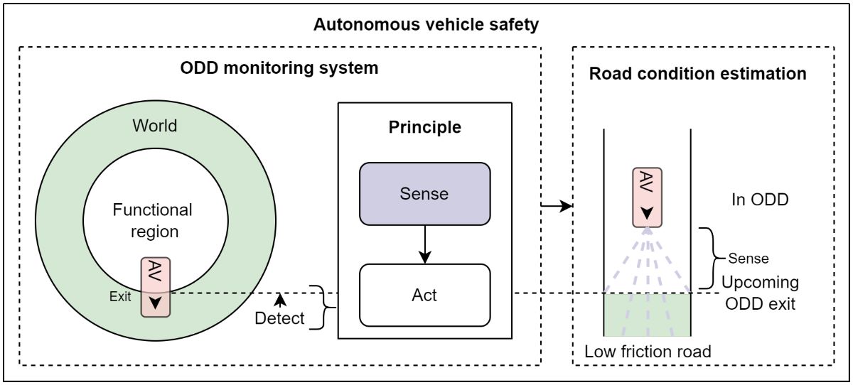
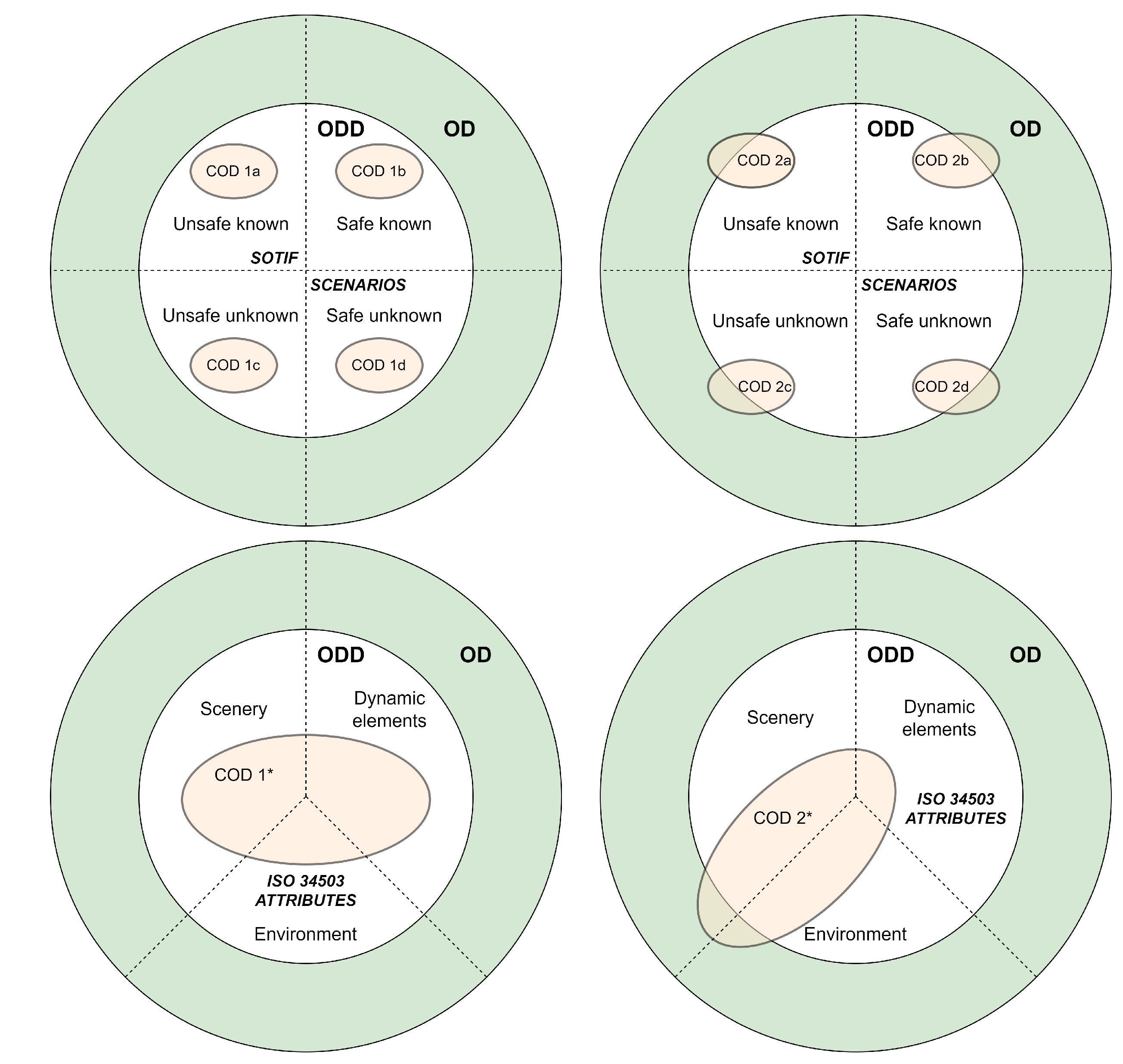
An ODD helps differentiate between potential functional regions of an AV, namely the real-world Operational Domain (OD), the desired functional region Target Operational Domain (TOD) and the real functional region Current Operational Domain (COD). ODD, COD and TOD are all subsets of OD, as can be visualized in Figure 1. An exception is naturally an AV at L5 of autonomy, where its ODD equals OD. Additionally, TOD is a subset of ODD, while COD is the state of the environment at a particular time instance. COD should be a subset of ODD at all times, but is not always the case in reality. An AV is designed and verified for a particular ODD, and it should be ensured that the AV is not subjected to any risks not accounted for within the ODD [2]. It is important that this restricted area is enforced for AV’s safety, but it is still possible that it may not be enforced all the time, leading to an unintended and forced exit from the ODD [3], or COD ¬ ODD. It is crucial to detect this exit in real-time using an ODD monitoring system (OMS).
ODD exits can be visualized on a chart from two perspectives: the SOTIF perspective or the ISO 34503 perspective (Figure 2). ISO 34503 is a state-of-the-art (SOTA) taxonomy to create an ODD [9]. SOTIF divides possible scenarios into safe and unsafe, further categorizing both into known and unknown. It suggests requirements-based testing for the unsafe known scenarios and scenario-based testing [10] for the unsafe unknown scenarios. An ODD exit could happen in any of these four cases, and is visualized by the COD 2a, 2b, 2c and 2d partially overlapping on the region of OD.
Understanding ODD exits from an ISO 34503 perspective is straightforward. ISO 34503 divides the attributes needed to define ODD into three primary categories: scenery, environment and dynamic elements. Scenery includes the static elements, the environment consists of weather, illumination and connectivity details, and dynamic elements are the moving objects around an AV. A COD, in this case, is always a combination of all three attributes ( C O D 1 * ). The COD instance 2 * in which the ODD exit happens, partially overlaps over OD from the side of scenery and environment. This implies that an ODD exit occurs due to a change in combination of scenery and environment attributes for which the AV was not designed [11].
ODDs are still quite restricted when it comes to weather-induced conditions and monitoring ODD exits in this category needs further exploration [12]. A special case of such exits ( C O D 2 * ) are these weather-induced conditions changing the frictional state of the roads. Monitoring the road is crucial because it is the primary area where AVs are permitted to travel. Ensuring that the road is safe and navigable directly impacts their overall safety and efficiency. Weather changes, especially winter-induced conditions on the road, lead to reduction in friction between the road and tires [13]. To tackle this reduced frictional situation, an advanced level of combination of perception, trajectory planning and control behaviour is required by AVs, but for which they are currently unequipped, thus endangering its overall safety [14,15]. Moreover, the perception has to be done quite in advance and in contactless form to give sufficient time for the AV to do a minimum risk maneouver (MRM) and go into a minimum risk condition (MRC).
Between 2019-2022, there were a total of 112,146 accidents in Germany, that involved personal injury. Out of those, 48,180, which amounts to 43%, were due to slippery roads due to rain, ice and snow [16]. These incidents occurred under the decision-making of a human driver, a level of judgement and experience that AVs have yet to fully achieve. Research on object obstacle avoidance on the roads has been at the forefront for many years with splendid results. while research on contactless road condition estimation (RCE) has largely remained in the background [17,18]. The necessity of implementing contactless RCE as a use case of OMS to increase the overall safety of AVs is becoming more and more clear, and the research is catching up.
This article is divided into two parts. The first part concentrates on few key strategies on OMS that were developed in recent years, the challenges encountered, and a framework visualization that can guide the development of OMS. The second part examines the topic of RCE, presenting a timeline of research efforts, highlighting current challenges, and concluding with a factual comparison of two SOTA RCE datasets.

2. ODD Monitoring System

The duty of an OMS is to provide advance warning to the AV about an impending ODD exit. Depending on the level of autonomy, the OMS should either trigger a takeover request [19] for a human operator (L3) or initiate a Dynamic Driving Task (DDT) to ensure the AV transitions to a state of MRC (L4). An ODD exit has to be detectable for the AV’s perception system to detect it in real-time. This detectability depends on several factors. For instance, the ODD exit should have a defined trigger point, and the AV must be equipped with appropriate sensors capable of perceiving this trigger point through a perception data processing algorithm. The next subsection reviews the previous work in the field of OMS. To conduct the literature review, high-level attributes hierarchy outlined in ISO 34503 were referred.

2.1. Related Work

In 2017, the authors in the work [20] designed a safety module for AVs that monitors its surroundings, particularly road networks and moving obstacles. Safety agents identify hazardous situations based on input from AV’s perception module. A recording component logs both the location and specific safety condition that was breached and saves the location coordinates on pre-loaded road networks map. When hazard thresholds are exceeded in a specific region, due to an accumulation of recorded safety breaches, the system triggers appropriate behavioral adjustments from a list of fallback strategies, aiming to preemptively address recurring safety breaches. For instance, if the AV frequently encounters situations where it fails to maintain a safe distance from another moving object due to that other object’s behaviour, the system will automatically reduce the AV’s speed at that location to ensure that a safe distance is maintained.
The work of [21] marked a significant milestone in research of OMS. The authors propose a mapping of system functionalities with the ODD definition, and introduce the concept of a Restricted Operational Domain (ROD). A variable ROD, a subset of ODD, is maintained in real-time according to the degraded functionalities of the different sub-systems in an automated driving stack (ADS). These sub-systems are monitored by a centralized system health monitor. By mapping the degraded functionalities to the ROD, the ADS ensures that it always operates safely within this ROD. For example, if there is an impairment in the front camera, all elements of the ODD that need to be detected by the front camera will be removed from the ROD, reflecting the degradation of functionalities and the subsequent shrinking of the ROD. Additionally, the ROD is monitored by comparing pre-defined vehicle parameter thresholds with real-time parameters. In the worst-case scenario, if an unwanted ROD exit is imminent and cannot be contained, a DDT fallback strategy is triggered.
In [2], the importance of quantifying and mapping use cases (UCs) ,CODs and ODD definition to each other using a world model is emphasized for detecting ODD exits. The derivation of an AV’s requirements from a generic UC definition is quite complex. For instance, if an AV is designed to operate only during the daytime, it is unclear from a UC definition whether a strategy to detect eclipses is required. The proposed process involves translating broad, high-level scenarios into specific operational conditions and constraints that the AV must adhere to. Mapping UCs to ODD, and both external and internal CODs, ensures that an ODD exit is detected in real-time. Inputs for interpreting a COD could come from perception sensors and pre-stored information such as weather reports, accident statistics, institutional reports and map data. An example to understand this method is that the velocity difference during overtakes could be analyzed and quantified using overtaking data from a certain time period and location, and an ODD exit can be predicted accordingly at those locations.
The integrity of 2D laser-based localization algorithms such as odometry, map-matching and SLAM was monitored in the work in [22]. The authors proposed a method that processes the 2D raw input from laser sensors before it enters the localization module. The monitoring algorithm divides the 2D input into grid patches and decides through a classification algorithm, whether distinguishable information needed to localize the AV is present in that patch. The system then warns the localization module in real-time about potential failures. For instance, distinguishable information could be a manually annotated stone. The framework was validated by the authors in a simulation environment from CarMaker. While 100% of instances, when "In ODD" was predicted, were accurate, only 23.54% of instances, when "out of ODD" was predicted, were correct.
The work of [11] was one of the first significant attempts to define a unified ODD monitoring framework, that addresses all three high-level attributes stated in ISO 34503. Their work discusses how an OMS can mitigate SOTIF risks by monitoring crucial attributes through three different modules. For weather monitoring, the authors derive a function to estimate safe speed of AV from rain intensity values. The maximum detectable distance of a LiDAR is derived from the rain intensity values, and on the basis of this distance value, the safe speed is calculated. The intensity values used here are not measured in real-time but taken from previous experiments on rainfall intensities. The digitization of traffic signs into logical definitions, containing trigger conditions and required behavioural responses, is used to monitor vehicle behaviour. Road defects are monitored by identifying outliers in the fitted LiDAR point cloud on road surfaces, which in turn prompts behavioural responses. While road slipperiness is mentioned as a concern, it is not directly addressed in the work.
A two-stage road topology monitoring method is proposed in [23], leveraging the concept of out-of-distribution (OOD) analysis in deep learning (DL). OOD analysis examines the behaviour of ML networks when they encounter data that deviates from training set. This concept is used to identify road structures that fall outside the ODD. In the first stage of the framework, a ResNet18-based CNN is trained with road topology structures within the ODD. The network learns prominent features and classifies the topologies into 6 different types of road structure. In the second stage, the learned feature space is compared with the feature space of test data and an OOD score is estimated to determine if the road structure is out of ODD.
The authors in [24] address the challenges of inadequate ODD definitions for designing OMS, the lack of efficient verification methods for ODD-based monitoring modules, and the complexity of logical expressions in SOTA OMS, by implementing their idea on the case of lane-keeping system in AVs. They propose a complete workflow, including ODD definition, a runtime monitoring module, and the required verification strategy. A causal approach is first used to analyze the dependency of the ambiguous perception-related ODD elements on lane detection accuracy, while a phase-plane stability analysis is performed to define the control-related ODD elements. The lane detection algorithm is monitored,and when a new COD is detected,that lies outside the ODD, a perception degradation strategy is activated. When necessary, the responsibility for lateral control is shifted to AV’s safety system. For the perception degradation strategy, radar is used as the main sensor to calculate the distance from other moving obstacles.
Convolutional Neural Network (CNN)-based algorithms are increasingly becoming more common in AV stacks, particularly at the perception level. It is crucial to maintain the ODD for these algorithms due to their black-box nature, which makes it unclear when they might fail. A runtime monitor for such kind of algorithms is proposed in [25]. The network correlates a diverse input feature space to pre-defined safety specifications and predicts an ODD exit when there is a risk of these safety specifications being violated. An analysis of Deep Neural Network (DNN)-based perception algorithms runtime monitoring is presented in [26]. This analysis compares monitoring methods suggested by the ML community, those proposed by the formal methods community, and methods that do not require analyzing the DNN itself. The reliability of DNN-based perception algorithms in AVs under varying and foreign conditions is further addressed in [27]. The DNN’s performance on aggregated sensor data for known and corresponding OCs is recorded, and quality models are generated. Sensor properties and redundant information from multiple sensors are also considered. In the next stage, a reliability error is estimated in real-time from the learned quality models. Based on this reliability error, adaptation tactics are undertaken at perception level to ensure the robustness of these perception algorithms to varying OCs.
Important works in OMS are summarized in Table 1, according to the year, the primary attribute they address, and the core concept of their framework. From the analysis of the detailed works above, it is evident that mapping OD, ODD and COD to safety specifications is crucial for substantiating the safety case for an AV. This mapping ensures a more effective and comprehensible test strategy, and facilitates the design of an OMS. Although various researchers have addressed the issue of OMS, a clear and concise framework that is easy to understand and exclusively based on defined ODD attributes is needed. Research on monitoring DL-based perception algorithms in real-time is progressing, while weather-based ODD exits have not been explored in detail.

2.2. Framework

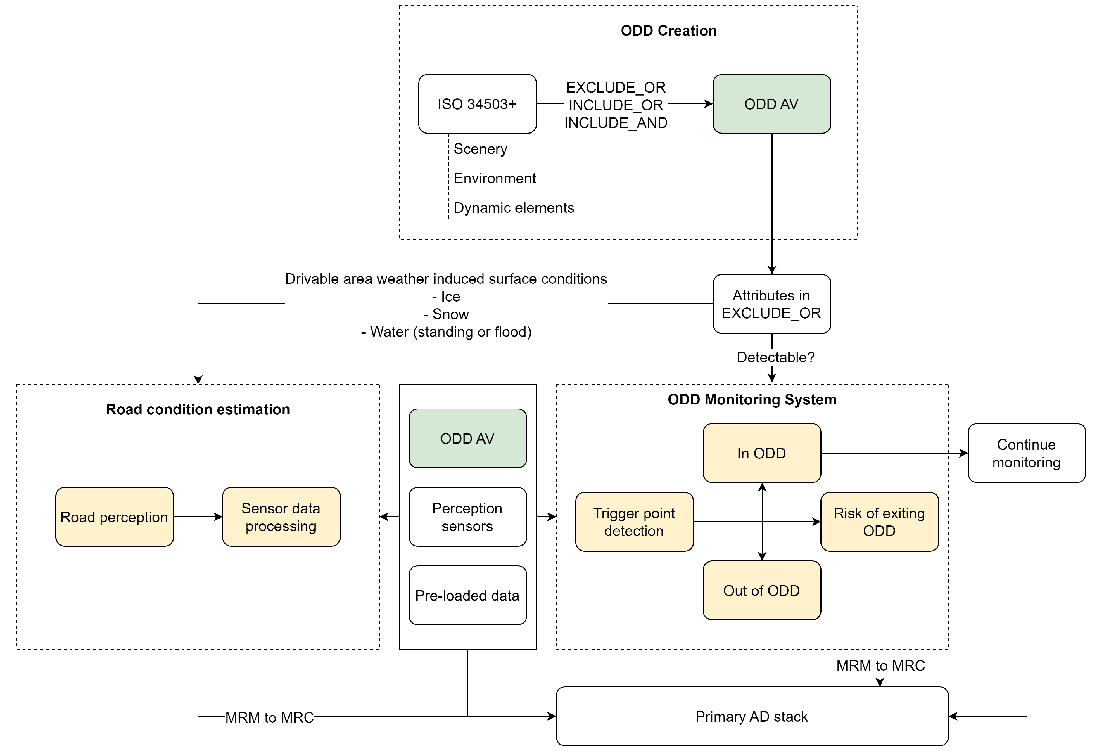
An ODD exit detection framework that incorporates ODD specifications and perception sensor data is illustrated in this subsection (Figure 3). To determine the trigger points, the attributes excluded from the ODD definition of an AV, as per ISO 34503, are used as the foundation. Within the OMS framework, an AV can exist in one of three possible states: within ODD, at risk of exiting ODD, and out of ODD. The risk of exiting ODD involves a transition from one COD within the ODD to another outside the ODD. This transition must be detected by the OMS to prevent the AV from reaching the second COD state.
For the specific use case of RCE, the excluded attributes in question include weather-induced conditions such as water, snow and ice on the roads in different capacities and forms. In this scenario, detecting the trigger point during the transition is primarily a perception problem, with the control module remaining unaffected. This implies that primary ADS’s control module remains within its ODD and can still be relied upon to execute maneuvers. However, if the AV has fully exited its ODD, the controller has also exited its ODD, necessitating the requirement of different approach to handle such exits.
The detectability of the trigger point is decisive for designing an effective and robust OMS. Some trigger conditions are straightforward and easy to detect, primarily based on the static scenery elements, the ego vehicle’s parameters, and those of the surrounding vehicles, while other types require a more thorough investigation to design detectable ODD exits. To the authors’ knowledge, the RCE as a special use case of OMS has not been previously addressed. The next section will explore RCE and its implementation using computer vision methods, through which, aiming to address the limitations of weather-related ODD for AVs and facilitate their deployment in more extensive ODDs.

3. Contactless Computer Vision-Based Road Condition Estimation

The responsibility for detecting anomalous road conditions lies with the driver in human-driven vehicles, while for AVs, the onus shifts to the perception system within the ADS [30]. While the behavioural response required for managing slippery road conditions is consistent between manned and unmanned vehicles, the key deciding factor is the difference in the perceptual capabilities.
The goal of an OMS is to replicate the perceptual capabilities of a human driver in detecting oncoming ODD exits. ODD exits in the context of road conditions could include road damages or the reduction in frictional state of the roads [30]. Road damages encompass potholes and cracks. The authors of [31] conducted a survey on these types of exits, highlighting how DL has surpassed conventional ML algorithms. This section, however, delves deeper into the science behind the ODD exits triggered by reduced road friction due to rainy and winter weather conditions. A timeline of research is presented, the SOTA methods are then detailed, followed by a discussion of contemporary challenges and potential directions for finding concrete solutions.

3.1. Literature Review

A clear perception of the road, followed by processing and correlating the knowledge obtained with the existing frictional state of the road, is necessary for RCE. This state knowledge is then passed on to the controller that plans the applicable behavioural reaction. Various parameters in this workflow determine how effectively the RCE functions. Sensory perception of the road can be achieved in a contact form through traditional mechanical methods or using principles of capacitance, magnetorestriction, piezoelectric resonance, fibre optic or flat film resonance, but the necessity to reduce maintenance costs and achieve real-time RCE has led to the emergence of contactless sensors [17]. Contact sensors are directly installed on the road[32], but primarily for purpose of winter road maintenance. In case of an AV, the tires are the only parts in contact with the road. While friction estimation using tire slip has been explored, it requires the AV to first make contact with the affected area [33], which undermines the whole purpose of alerting the AV before it comes in contact with that area. This makes the development of contactless RCE crucial and pivotal. Furthermore, the ramifications of failing to detect the affected road part amplify the importance of necessity of a prior warning. This prior detection allows for timely behavioral adjustments, reducing the probability of hazards and accidents occurrence and enhancing the overall safety of the AV [34,35].
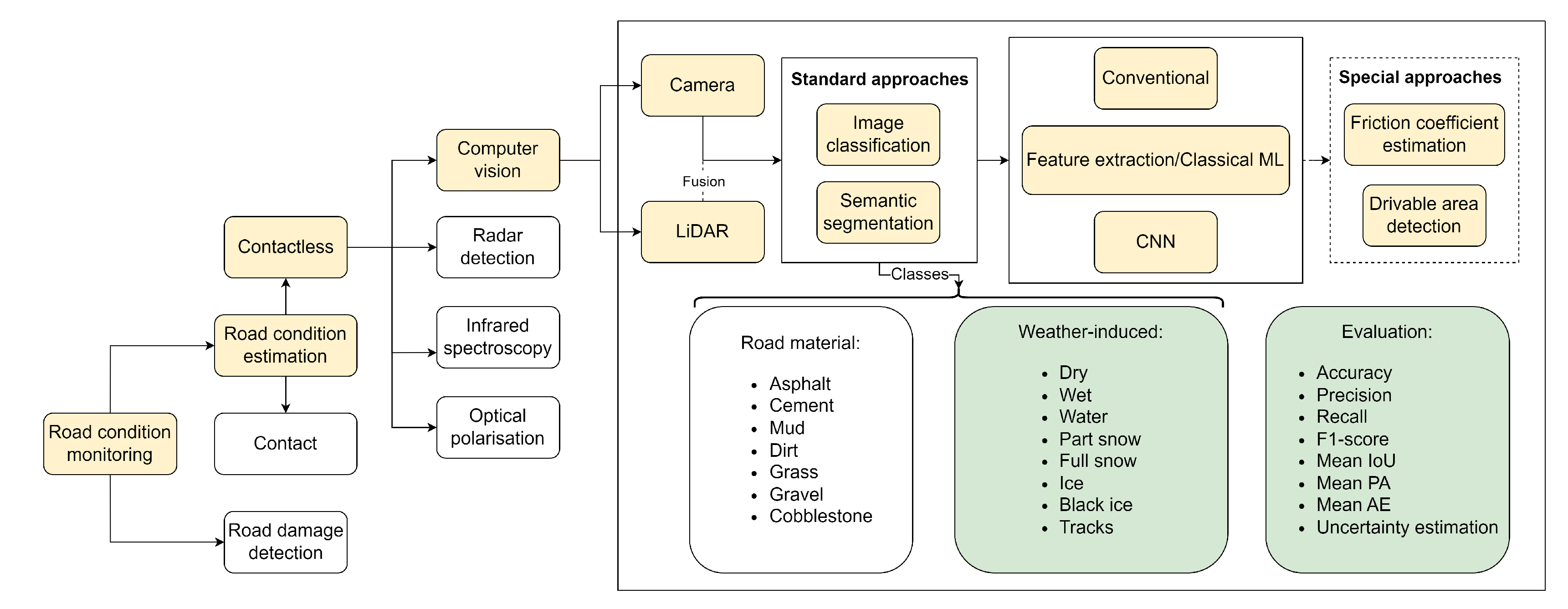
The choice of sensory perception medium decides the trigger point (Section 2). In the case of contactless RCE, the perceptual power of the sensor is crucial and also determines the effective range at which RCE functions. A balance must be maintained between maximizing detection distance without losing critical features. Sensors and sensing principles work hand in hand, as outlined by the authors in [17], who categorized contactless RCE methods into infrared spectroscopy, optical polarisation, radar and computer vision. Near-infared LED has been employed to differentiate between dry, snowy, and icy surfaces, utilizing varying light scattering behavior upon incidence on those surfaces [36,37,38]. In 2012, the difference in permittivity properties of ice and water at lower and higher frequencies was used as the principle for capacitor-based ice layer detection [39]. Camera-based road perception has gained prominence in recent years, although its roots trace back to 1998 when researchers from Sweden utilized images to differentiate winter road conditions [40]. Over the years, resolution of the images has improved, accompanied by advancements in feature extraction algorithms and classical ML techniques, making cameras increasingly common in RCE applications [35,41,42]. Being an integral component of an ADS as the standard vision sensor, and its affordability and availibility at a reasonable price further enhances its practicality [43]. Cameras are adaptable for use not only within AVs but also alongside roads to minimize occlusion issues [15]. Specifically for RCE, their utility has been also occasionally combined with other vision [44] and non-vision sensors [14] to improve the detection accuracy. The advent of CNN-based feature extraction techniques has now positioned camera-based RCE among significant topics of research [15].
Correlating the exact friction coefficient of the road directly from camera images is desired but not feasible. As alternatives, in the early years, researchers explored various strategies to address this challenge. Depending on the road material and type of weather-induced condition, a rough estimate of the friction coefficient of a certain road patch can be envisaged, and this knowledge can be used to group the road patch images into different classes, effectively conceiving an image classification problem [31,45]. An example of the process of road patch acquisition can be seen in Figure 4, where the real road image on the right-hand side is taken from the dataset of [41]. The camera fitted on the ego vehicle has a clear view of the road. A road patch extraction algorithm sends only the relevant part of the road to the RCE algorithm, thus reducing the computation required. Efforts have also been made to use pixel-level features for segmenting winter-induced conditions on the roads in the captured images. Practical approaches such as detecting drivable areas by leveraging identifiable features like trodden snow on the road have also been explored. In recent years, the research is slowly shifting to directly calculating the friction coefficient from image features. In Table 2, the most commonly used evaluation metrics are listed to help the reader better understand the different methods.

3.1.1. Image Classification

A significant breakthrough on RCE happened back in 1998 [40], when the researchers worked with a small dataset of 69 color images to differentiate between dry, wet, tracks, snow and icy roads. They selected the different statistical parameters of gray levels, and additionally the standard deviations of ratios of red and blue, and red and gray level as features. The features were then used to train a simple feed forward neural network, and the proposed technique achieved an accuracy of 52%. Distinguishing between wet and icy roads proved to be the most challenging, while between dry and snowy the least. During dataset preparation, the most significant challenge was the manual annotation of the images, particularly in correctly differentiating between wet and snowy conditions, as slushy conditions exhibited characteristics of both.
A purely mathematical solution was proposed in [34], which aimed to capture the vertical polarization intensity of different winter surfaces using block filters. The results were then enhanced using a graininess analysis, where the contrast between the original image and the blurred image was analyzed. This approach did not consider the road material and focused on conditions such as snowy, icy, wet and normal dry asphalt states. The polarization step was successful in differentiating snow with icy and wet conditions, but the graininess analysis failed to differentiate between all the three condition altogether.
An innovative classical ML approach was introduced in [46], which identified color as the most relevant feature for differentiating snow from dry roads. Using a set of 516 images, RGB histograms were extracted for small sub-images, and then concatenated, and used as feature vectors for differentiating between snow and bare roads while edge detectors were employed to differentiate between tracks from other classes, leveraging the presence of straight lines of tracks. The features were then trained using a Support Vector Machine (SVM) to achieve a maximum of 89% accuracy on images recorded from a drive recorder.
Existing public datasets were utilized effectively by authors in [35], in which they assembled 19000 road patches and used them to fine-tune ResNet50 [47] and InceptionV3 [48] models to differentiate between four road material types – asphalt, dirt, grass and cobblestone – and two road condition types – wet asphalt and snow. Color features proved to be crucial again for distinguishing between the classes, although the ambiguous texture nature of the defined classes led to several misclassifications. Among the models, ResNet50 performed the best, achieving an average accuracy of 92%.
The authors in [49] modified the ReLu activation function to prevent loss of neurons during training, addressing the issue of fluctuations in weights. The leakage from the negative axis of ReLU is taken into account in the training process, and as part of a 13-layer CNN, 1600 images are trained to classify between dry, wet, snowy, muddy and other roads. A test accuracy of 94.89% is achieved on 400 images.
The proof of ResNet50’s robustness in RCE applications was further strengthened in [50], where 28000 images from in-vehicle cameras were used to fine-tune 4 SOTA classification CNNs (VGG16, ResNet50, InceptionV3 and Xception) to predict bare, partly snow covered, fully snow covered, and unrecognizable conditions, achieving a maximum accuracy of 99.41% [51,52]. 4728 images from fixed roadside Road Weather Information System (RWIS) cameras were used to test the robustness of these models to external factors such as camera angle, illumination, distance, road topology and geometry.
In [53], the authors proclaimed surface texture as the decisive factor in RCE, while using computer vision methods. They employed circular local binary patterns to obtain the minimum value of grey level texture from the images, and also used grey level histogram as a significant first-level feature from a dataset of 1000 images. These features were trained on a random forest (RF) model and a custom VGG-based CNN TLDKNet, and the performance was compared. The CNN achieved 80% accuracy in distinguishing between road patches of high, medium and low resistance, outperforming the classical RF model by 20%.
RCE method using video data and a CNN-based feature extractor was developed in [54], and tested on a vehicle model to control the breaking behaviour. Although the proposed CNN was not the best fit for all types of braking systems, it was found to be effective for simple brake systems. The proposed method achieved an accuracy of 92% on a dataset of 1200 images with dry and wet conditions.
A new custom 33-layer CNN called RCNet was introduced in [55] and its performance was evaluated using seven different optimizers on a dataset of 20,757 images to classify roads as curvy, dry, icy, rough, or wet. The Adam optimizer is found to be the most suitable, and the computational efficiency of RCNet was reported to be superior to that of the model presented in [49].
Surface condition detection using images from RWIS and fixed roadside webcams was proposed in [56]. In a comparitive analysis between SOTA pre-trained CNNs AlexNet [57], GoogLeNet [57] and ResNet18, the latter ResNet18 was found to be the best performing to classify a dataset of 15000 images into dry, snowy and wet/slushy to achieve an average accuracy of 99.1% on a test dataset. The ResNet architecture triumphed again in [58], but this time on a dataset of 18,835 images from an in-vehicle camera. The classical ML models SVM and K-Means Clustering were compared with the CNN architectures ResNet50 and MobileNet, and ResNet50 demonstrated superior performance, achieving an accuracy of 98.1% for classifying dry, wet and icy roads.
Challenges in RCE during nighttime include the difficulty of reliably capturing road patches due to absence of sunlight. The available illumination sources are primarily headlights of ego vehicle and in some instances, ambient light from headlights of other vehicles and street lights. The presence of ambient illumination cannot be ensured all the time. Dry and snow surfaces, due to their rough texture, reflect light in all directions. In contrast, wet roads have a more smoother textures resulting in higher capturability only from the ambient lighting, while reflections from ego vehicle’s headlights are often scattered away from the camera. This dilemma is analyzed in [59] where 45,200 images collected at night time with and without ambient illumination are trained on SOTA classification architectures, SqueezeNet [60], VGG16/19, ResNet50 and DenseNet121 [61], and three custom CNNs. DenseNet121 outperformed ResNet50 by nearly 2% making it the most effective classifier of road patches for nighttime conditions.
A highly imbalanced dataset of 3790 images with broad labels for different weather and road conditions, including wet, snowy, dry and icy, was analyzed for RCE classification using SOTA CNNs and notably the Vision Transformers (ViTs) [62] in [63]. The ViTs have gained prominence for image processing in last few years. Unlike conventional CNNs, which evaluate relationships between every pixel in an image, ViTs process small patches, thus reducing overall computation time. In this specific work, ViT-B/32 model achieved a training accuracy of 98.66% while ViT-B/16 model achieved a slightly higher validation accuracy of 90.95%.
In a significant milestone for RCE, a wetness dataset (RoadSAW) was introduced in 2022 [41], accompanied by a baseline analysis on it using the MobineNetV2 architecture [64]. The choice of MobileNetV2 was driven by the need to balance the complexity of CNN networks with higher computational efficiency. This dataset, one of the first large-scale for RCE, comprises 720,000 road patches categorized into 12 classes with 3 road material types and 4 wetness conditions. The dataset attained an F1-score of 64.23%, setting the stage for further research opportunities and advancements in the field. In 2023, the same authors complemented the RoadSAW dataset with a snowy road patches dataset (RoadSC) [65]. This new dataset features 90,759 manually annotated images categorized into freshly fallen snow, fully packed snow, and partially covered snow. When combined with the RoadSAW dataset, the overall F1-Score improved to 70.92%.
Another large scale RCE dataset Road Surface Classification Dataset (RSCD) was introduced in 2023 [30], featuring 27 class combinations and a baseline analysis using the architecture of EfficientNet-B0 [66]. To enhance the robustness of the algorithm, a fusion technique based on Dempster-Shafer (DS) evidence theory is also proposed. The baseline analysis yielded an accuracy of 89.02%, while ablation experiments increased the training accuracy by 3% to reach 92.05%. On a test dataset of 1200 image pairs, the fusion approach reached an impressive accuracy of 97.50%.
To address feature redundancy and class imbalance issue in RSCD, the authors in [67] explored an innovative approach by modifying the RexNet network, a MobileNet-based CNN. A separate feature extraction convolution was introduced for low dimensional and high dimensional features which are then fused in a later stage, leading to the definition of a custom CNN classifier, Attention-RexNet. For the long tail issue in the dataset, a balanced softmax cross entropy is proposed. The proposed algorithm was unable to cross the baseline accuracy, yielding only 87.67%.
The authors in [68] combined lightweight ViTs, TinyViT and MobileViT [69,70], to leverage their ability of sustaining spatial information till they can be subjected to a late fusion that integrates the local and global characteristics of the images. Using RSCD, they developed a late fusion module that concatenates the feature maps and inputs into a simple classifier block. The choice of ViTs was motivated by their computational efficiency and suitability for real-time RCE estimation. A baseline comparison with the previous works is done and their model EdgeFusionViT was able to surpass the baseline results from [30] by achieving an accuracy of 89.76%. The generalization capability of RSCD and RoadSAW/RoadSC datasets are discussed in detail in the next subsection.
Two examples where the weather data was considered to enhance the classification accuracy are detailed next. In [72], the authors combined five weather variables – air temperature, relative humidity, pressure, wind speed, and dew point – with 14,000 images to classify road conditions as bare, partly snow-covered, and fully snow-covered. They first compared seven state-of-the-art CNN models on the images alone, then integrated the weather data using three classical ML models. After the fusion, the Naive Bayes Classifier marginally achieved the highest accuracy. Another instance of fusing the weather parameters was done in [14], where where 600 images are taken from an asphalt pavement in Northeast Forestry and The image features were combined with meteorological data and temperature data. an average precision of 95.3% was achieved to classify between the classes dry, fresh snow, transparent ice, granular snow and mixed ice.

3.1.2. Semantic Segmentation

Task of pixel level classification of winter-induced conditions on camera images was undertaken in [72]. The novelty of the work lay in the incorporation of cascaded dilated convolutions within the original encoder-decoder structure of U-Net [73], allowing the model to capture both local and global context information, thus leading to the development of a custom CNN D-UNet. The difficulty in identifying classes such as snow and ice was addressed by assigning higher weights to them during the training phase. Experiments conducted on a dataset of 2080 images demonstrated that the D-UNet model outperformed the original U-Net, achieving a mPA of 87.15% and a mIoU of 79.30%.
The authors in [43] introduce a new snow dataset with 11 pixel-wise annotated classes, consisting of both real and synthetic images. The snow cover in the real images was used to train a semantic map generator based on Pix2PixHD to generate snow semantic maps that were then transferred to images on Cityscapes [74]. The proposed method addresses the shprtage of datasets for solving RCE using CNNs. The performance of different SOTA pixel classifiers such as SegNet, ENet, ERFNet, ICNet and BiseNet [75,76,77,78,79] was evaluated on this dataset, highlighting the importance of synthesizing new images for effective training.
In [80], a dataset of 800 images consisting of black ice on the road was subjected to a classification with a bounding box and subsequent segmentation analysis using SOTA CNNs, Mask R-CNN-based structure R101-FPN1 and 3 variations of YOLO family [81,82]. In a clear weather on an asphalt pavement, the AP50 of the Mask R-CNN model was 92.5%, but it decreases to 54.6% for a foggy weather.

3.1.3. Drivable Area Detection

Also falling under segmentation problem, but approached in a different way by the decision of definition of class, the authors in [44] addressed the RCE by using camera and lidar data fusion to classify each pixel on the images as drivable or non-drivable. To achieve runtime-capable algorithms, they optimized the convolutional neural network (CNN) used in their previous work [83]. They experimented with seven different combinations of fusion, introduced synthesized fog noise on images and point clouds to test robustness, and compared their method with existing SOTA-based classifiers.
The pixel-level changes in images of different snow coverages on roads due to melting and driven tracks of other vehicles was considered in [12]. A histogram analysis of every image was performed. The extracted mean and variances of each RGB histogram distribution were used as features to feed into ML algorithms. The image level features were then averaged for a whole video for a video-level analysis. The image features were also combined with the daily Snow Water Equivalent measurements and six conventional ML algorithms were tested to classify conditions into no snow, standard snow and heavy snow. RF yielded an impressive accuracy of 95.63%. In a subsequent work [84], the authors proposed a segmentation method to identify driven tracks using both classical ML methods and variations of U-Net architecture. On a dataset of 1500 images, the Recurrent U-Net model was found to be the best performing with an accuracy of 89%.

3.1.4. Friction Coefficient Estimation

One of the first approaches to correlate the image features with a friction coefficient was presented in [33], where the authors designed a two-stage classifier using a dataset of 5300 images from a vehicle’s front camera. In the first stage, images are classified into dry asphalt, wet/water, slush or snow/ice, using a CNN SqueezeNet and a feature-based model. The SqueezeNet-based model achieved the highest accuracy of 97.36% by learning features from sky and the surroundings. In the second stage, the classified road patch is divided into 5x3 sub-patches, and each patch is regressed to a value between 0 and 1, 0 being for dry and 1 being for snow, yielding a probabilistic matrix. Finally, a rule-based model classifies the patches into low, medium or high level of friction. The overall method achieves an accuracy of 89.5%. Although, exact friction coefficients were not estimated, this work uniquely divided images into smaller patches for enhanced feature correlation between image features and road frictional state.
A consequential contribution for RCE was done in [18], where also the authors introduced a RCE dataset, Winter Road States. They addressed the issue of open-soruce unavailability of most datasets that were used for RCE previously. 5061 images were collected from famous AV datasets and were annotated as – dry, wet, partly snow, melted snow, fully packed snow, and slush. A mapping is also established from road states to approximate friction coefficients. In a subset of 2007 images, the drivable area is annotated pixel-wise. The original dataset is trained on 6 previously mentioned SOTA CNNs. An auxillary network performs the segmentation task on the images to identify the drivable area, concentrating mainly on the road features, and this segmented map is transferred to the classification results. Once again, ResNet50 as the base structure achieves the highest accuracy of 86.53%.
Vehicle parameters are synchronized with the results from RCE part in [85] to have a unified effect on the control module and acquire the tire road friction. In the RCE part, there are two segments: semantic segmentation for reducing the detail, and then a ShuffleNetV2-based road condition estimator [86]. This idea used here is similar to [18]. Semantic segmentation part is trained using 500 images from Cityscapes. For the classification part, 8000 original images were collected for 8 different classes: dry asphalt, wet asphalt, dry cement, wet cement, brick, loose snow, compacted snow and icy and an accuracy of 97.9% was achieved. In parallel, an unscented Kalman Filter estimates the tire-road coefficient from the vehicle dynamic parameters, and the confidence values from both visual and dynamic sections are fused together to get a unified tire-road friction coefficient.
The creators of RSCD further extended their analysis on their dataset by attempting to estimate the exact friction coefficient of the road patch [45]. In the first stage, the images are classified into the 5 different classes – dry, wet, water, snow and ice – using an EfficientNet-B0 network, achieving a top-1 accuracy of 94.84%. In the second stage, the predicted class is mapped to a friction coefficient range using Gaussian kernel functions. Misclassifications are handled in the secondary stage with a filter to converge the faulty friction values to desired range.
Another significant work in estimating the friction coefficient from images is presented in [15], where the authors propose a regression approach to estimate a scalar frictional value from image features. The dataset used included 48791 images, captured from roadside cameras, with corresponding grip factor values. Feature extraction happens in parallel using a DINOv2 structure and a custom CNN structure, with the features concatenated at the exit. They are then further passed on to a fully connected NN, ending with a sigmoid function, to produce a scalar value. The evaluation is compared with other SOTA CNNs, and their custom architecture was found to be the best performing a MAE of 15%.

3.2. Discussion

A summary of the survey of SOTA can be seen in Figure 5. The works of [17] and [31] were partially referred to create the figure. The results from different RCE algorithms are listed out in Table 4, and it is evident that the research has shifted towards CNNs for capturing the relevant features specific to RCE. Classification of the road patch images is the most common approach. In the early days, ResNet50’S architecture was found to be the most suitable, also providing the best results. As the focus later shifted towards achieving better computational efficiency, keeping in mind the real-time implementation of RCE in AVs, networks such as EfficientNet-B0, MobileNet and ViTs were adopted. Additionally, the importance of RCE results in affecting the vehicle dynamics has also been considered in few research efforts, by converting classification results into a single frictional value. Despite challenges like the lack of friction coefficient measurements with the image datasets, researchers have navigated the issue by assuming the frictional coefficient ranges of different winter conditions.
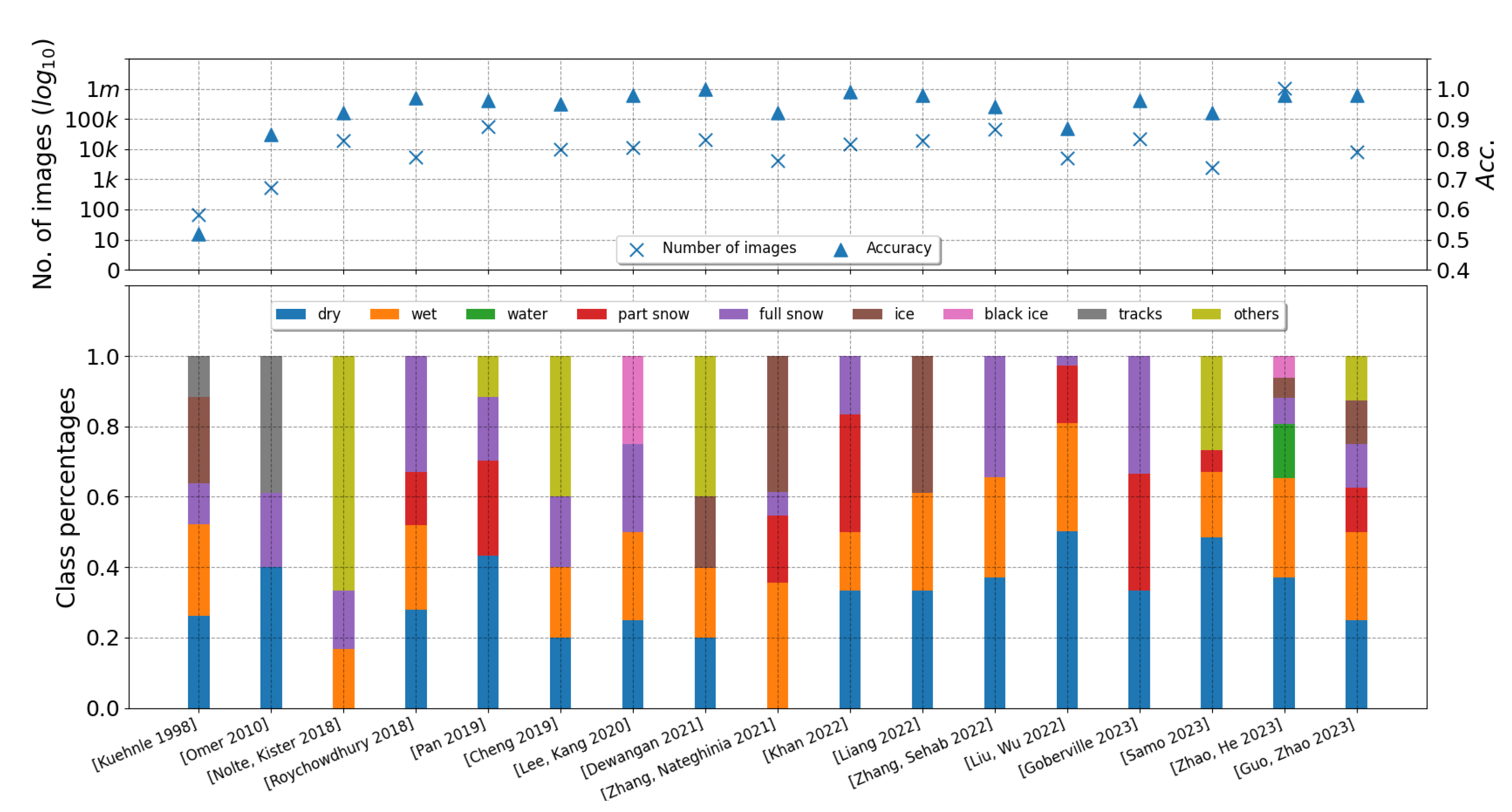
The issue of class imbalance among the datasets used in different algorithm has been identified. The defined classes in the datasets are often restricted to the location of dataset collection, weather conditions and annotation methods. Annotation is manual in most cases. This class imbalance prevents a direct comparison between different proposed algorithms. Two major factors for defining classes are the road material and the weather-induced conditions, as also analyzed separately in [31]. The class definitions also depend on how the dataset collector perceives the different winter conditions. For example, [65] introduced a dataset with categories such as fresh fallen snow and fully packed snow, whereas other datasets simply have a single class snow. Moreover, partially covered snow could result from snowy surfaces driven over by other cars, leading to tracks, that are separately defined as a class in [40,44,46,84]. On the other hand, partially covered snow could simply be due to less quantity of snowfall. Ice and black ice [80,87,88,89], which are significant causes for accidents, are often not included in most datasets, although a few works define slush. Another factor to be considered here is the effect of combination of road material and weather-induced conditions as a single class on the CNN algorithm [30,35]. Some works have provided an even simpler distribution of classes between drivable and non-drivable [44]. In [55], the authors have 3 weather-induced conditions-based classes (dry, ice, and wet), one road material-based class (rough), and one road formation-based class (curvy), and images from all these classes were trained together on a single CNN. The question arises: how similar are two classes from different datasets, and can a uniform annotation method be defined? A distribution of images across different classes used over the years in few of the important works is presented in Figure 6. To plot this figure, nine main classes were decided and number of images from individual datasets grouped into these 9 main classes. This assignment can be seen in Table 3.
Datasets play a crucial role in computer vision methods, especially when deep learning is involved [35,43]. Limited training data has always been an issue [68]. The failure of most ML algorithms is due to the difference between the data they were trained on and the data they receive at runtime [90]. Most AV datasets generated in winter were not collected with RCE in mind but rather to assess the performance degradation of vision sensors [74,91,92,93]. Moreover, the high costs involved in collecting these datasets are a deterrent.
Collection of datasets is followed by its annotation, especially for ML algorithms, which also costs money and time. While road material information can be accessed from government records, the weather-induced condition is mostly manually decided by the data collector. The annotation in [65] is done using Mobile Advanced Road Weather Information Sensor (MARWIS) [94], that calculates the water film thickness. This is one of the first datasets where the annotation is not done manually. Varying degrees of wetness leading to significant variations in driving behavior was taken as the reasoning for annotating the images in such a way. For semantic segmentation, annotation is needed for every pixel in the camera images, not only for winter-induced conditions but also for general objects. Similarly, for drivable area detection, the drivable area must be marked on the images. Again, this is based on the intuition of data collector, without any knowledge of the actual friction coefficient of that drivable part. In case of tackling RCE by estimating friction coefficient, they should be measured during data collection, and research in this area is still sparse. To save costs, one possibility is to create road patch datasets from existing datasets, provided their camera data offers a clear view of the road ahead . The rough labels provided could also be inherited, saving costs on labeling and annotation [95]. Simulating the road patches or segmented images is another option to save time and money, though it may lack realism [43].
Evaluation parameters involved in classification or segmentation problems not only provide an idea on the performance and robustness of the respective algorithms but their right selection could also help to estimate the relevance and worthiness of a dataset. For the classification tasks, accuracy is found to be the most common evaluation metric. Accuracy could also be misleading in case of unbalanced datasets or small datasets, especially in this kind of problem, where it is necessary to also compare the classes used. The relationship of number of images in each classes in datasets, total number of images, and the accuracy achieved on them can be seen in Figure 6, for few important works. The accuracies are mostly over 90%, but for varying number of images and classes. In [56] and [89], the authors achieve an accuracy of more than 98% but on a relatively small dataset of 15000 and 11000, respectively. Additionally, there exists also a class imbalance between the both. In certain cases, multiple winter conditions yielded similar confidence numbers, thus making it a challenge. The top-N accuracies help here to evaluate the classes that have a high confidence value but not the highest due to uncertainty. The top-N accuracies, on the other hand, also distort the results by including predictions with very low confidence value. The confusion matrix serves as a better solution here to check how further away the misclassifications lie from their true class, and it is also the second most used metric, furthermore, yielding the precision, recall and F1-Score values [88]. Real-time results are paramount in RCE, so the time taken for the CNN to process a test image was also considered in [59]. For segmentation problems, the mIoU is found to be the most common evaluation parameter [43,72].
Another important evaluation metric here, especially considering the ramifications of a failed real-time implementation, is the uncertainty estimation of the datasets used to train the CNN. Although the research in CNNs has gone quite forward, the research on predictive uncertainty is still a hot research topic. A generalization capability analysis is required in addition to the usual metrics to assess the quality of datasets and the algorithms trained on them, to evaluate how well the algorithm performs on foreign data. This is important because the datasets on which the CNNs have been trained are not uniform and from different regions in the world. This generalization analysis is also important because, only so much can be done at datasets collection level. The analysis gives us an idea to differentiate between what has to be done at dataset collection level, and what has to be done at the algorithmic level. Due to the complicated nature of the dataset in [50], a sensitivity analysis was performed to check the model’s reaction to these variations in the input. The extent of deviation of the predicted class from the actual class was calculated using underestimation and overestimation error in [53]. Specifically when RCE is planned to be implemented in real-time and the vehicle behaviour has to be controlled from its prediction results, dealing with misclassification is very crucial to avoid an abnormal behaviour of the AV. Here, an analysis of misclassified predictions is paramount [30,35,45].

3.3. SOTA Datasets

Appropriate datasets are crucial for the success of any CNN algorithm. Two of the most recent and largest datasets for RCE are RSCD [30] and RoadSAW/RoadSC [41,65]. The latest version of RSCD, released in 2023, contains 1 million road patch images categorized by three parameters: road unevenness, road friction condition and the road material, with further divisions into subclasses. It is the largest RCE dataset from Asia, whereas most previous datasets and related research are based on Europe and the USA [31]. Conversely, the RoadSAW dataset, initially released in 2022, features three types of road materials and four levels of wetness. Originally aimed at addressing road wetness estimation, the dataset was expanded in 2023 to include road patches under snow conditions (RoadSC), thereby creating a more comprehensive dataset for RCE. A factual comparison between the two datasets can be seen in Table 5.
RSCD contains more images overall compared to RoadSAW/RoadSC, but the latter includes images of similar classes in multiple sizes and distances from the camera. In RSCD, road patches sized 360 x 240 pixels are extracted from the area in front of the tires, ensuring two road patches from a single camera image. Conversely, in RoadSAW/RoadSC, the road patch is extracted from the middle of the road. The road materials mud and gravel are unique to RSCD, while cobblestone is unique to RoadSAW/RoadSC. The inclusion of these road materials as classes makes both datasets generalized in different capacities.
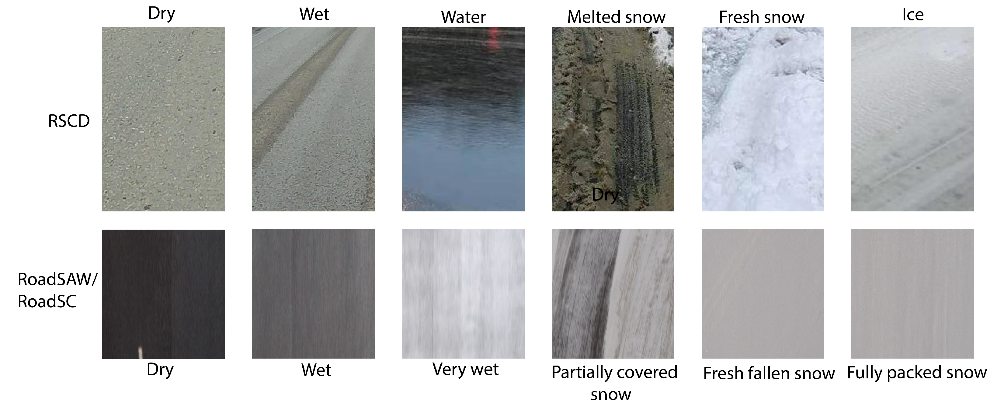
For wetness conditions, RSCD has manually annotated classes, whereas in RoadSAW/RoadSC, annotation is done by calculating the water film thickness using the MARWIS and categorizing the images into four different ranges. Images exclusively from RoadSC have been manually annotated. For winter-induced surface conditions, For winter-induced surface conditions, RoadSAW/RoadSC includes only snow-induced attributes, while RSCD also includes ice. Although "driven over snow" or "snow on the road with treadmarks" are not explicitly defined, the attributes "melted snow" and "partially covered snow" could partially denote these conditions. "Melted snow" could also denote black ice when it hardens, which is not separately mentioned in either of the datasets. Example of road patches for different winter conditions are shown in in Figure 7. It can be seen that the creators of RoadSAW/RoadSC calibrated every image to a bird’s-eye view level.
As seen in SubSection 3.1, RSCD has already undergone several analyses, achieving a maximum baseline accuracy of 89.76% using a ViT, as reported in [68]. In this section, we will focus on the work done on these datasets to assess their generalization capabilities. One way to do this is by developing methhods to handle misclassifications, as it is crucial to address them, especially in real-time implementation. To reduce the impact of misclassifications on real-time dynamic behaviour of AVs, the authors in [30] adopted a multi-sensor fusion approach to handle image noise. Based on the DS evidence theory, three partially overlapping images of the road are captured at a single timestamp. Conflicts between the images are evaluated to determine uncertainty, and a fused classification confidence value is generated. On a test dataset of 1200 images, this fusion method increased the overall classification accuracy to 97.50%. In [68], to test the model’s robustness, the authors trained it on only 2% of the entire RSCD dataset, achieving an impressive accuracy of 76.89%.
For the RoadSAW dataset with 12 classes, limited analysis on classification performance has been conducted so far. The authors established the baseline results, attaining an F1-Score of 64.33%. It was observed that as the distance of the road patch from the camera increased and the patch size decreased, the F1-Score diminished. Furthermore, the effect of emergence of noise in images leading to aleatoric uncertainty and epistemic uncertainty arising from model inadequacy due to insufficient training data, were both captured using Deterministic Uncertainty Quantification. Visualization of this estimation was performed using Area under Receiver Operator Curves (AUROC) scores, which indicated poor performance of the model on wet cobblestones, while on asphalt and cement, it was decent. The F1-Score from the implementation of the fine-tuned MobilNetV2 network on close-to-distribution datasets resulted in a very low F1-Score of 0.78% for wetness estimation alone. Combining RoadSC with RoadSAW increased the overall F1-score by 9% (from 61.60% to 70.92%) for a specific size and distance of road patch. However, AUROC scores decreased when the CNN was trained on all 15 classes, likely due to feature collapse.
This subsection intends to establish the importance of these two RCE datasets for future research. The generalization analysis on them also provides a foundation for evaluating future RCE datasets, not only based on common evaluation metrics but also by exploring new metrics that address the inadequacies better and offer a more genuine evaluation.

4. Conclusion

This study explores a pertinent challenge in the field of AVs: monitoring their operational boundary using an OMS. Maintaining the functional region for an AV at all times is not feasible, making OMS increasingly essential to detect potential ODD exits and thus enhance overall safety.
Several significant attempts to define an OMS were reviewed in this study, with ISO 34503 consulted to differentiate between various approaches. It is evident that research on OMS has primarily focused on monitoring the scenery and dynamic elements around the AV. The presented frameworks are either generic, applicable to any sub-modules of an ADS, or developed using special use cases. Incoming data from vision sensors, along with vehicle parameters, are mainly used as inputs to OMS. Furthermore, researchers have emphasized the importance of monitoring perception algorithms, particularly due to increased use of CNNs and their corresponding black box nature. Predicting the malfunctioning of such algorithms is challenging, and any such events could potentially lead to mishaps. Another observed trend is that ODD monitoring strategies often involve correlating sensor values with COD instances and learning from the past safety impairments to predict future impairments. This highlights another contemporary challenge: ODD and OD are not defined clearly enough for machines to differentiate between them easily, also making it harder to define the OMS. It also became clear from the study that weather-related elements in an AV’s surroundings have not been extensively addressed or considered within the scope of OMS. This study addresses these challenges by illustrating a general framework for designing and developing an OMS, especially for weather-related ODD exits. The framework recognizes that every ODD exit has a trigger condition. The defined trigger condition should be detectable and depending on the criticality of the ODD exit, the relevant trigger conditions can be prioritized for monitoring. To develop the detection algorithms, trigger points must be examined in detail, possibly extending beyond the scope of AVs and OMS.
In the next part of the study, trigger conditions for ODD exits due to reduction in road friction due to weather conditions were explored. The importance of computer vision-based RCE for estimating road friction in advance was established, with cameras identified as the most suitable sensor for this task. The study outlines a chronological progression of efforts on RCE using camera images, from classical ML algorithms from two decades ago to SOTA CNN-based feature extraction techniques. The study also surmised that initially RCE was approached as a classification problem for road patches. As CNNs gained prominence, architectures such as ResNet along with few custom CNNs, known for their superior image feature extraction capabilities, became popular for RCE tasks. Laetr on, with the increasing need for real-time implementation, architectures that prioritized computational efficiency, like EfficientNet and ViT were starting to be preferred. The approach of classification, when applied in real-time, must also address challenges such as misclassifications, which can lead to significant deviations from the ground truth and cause anomalies in real-time control modules. Few works also focused on segmenting weather-induced conditions on the images, providing pixel-wise information on road friction. Given that a scalar frictional coefficient value is more crucial for real-time RCE implementation, recent efforts have shifted towards correlating image features with scalar frictional values, yielding impressive results. However, research remains limited, as many datasets lack detailed frictional coefficient data, leading some studies to assume coefficient ranges. Nonetheless, it is evident from the study that this is the definite way to go forward.
Further challenges that were identified include the lack of large and comprehensive datasets for RCE. Although the datasets are diverse, manual annotation of each image and class imbalance between them make direct comparisons unfeasible. Evaluation methods for datasets and algorithms were also studied in detail in this work, establishing that generalization analysis of the datasets is as important as the CNN implementation. It is crucial to understand how a model trained on a dataset from one part of the world will perform in different regions. Furthermore, algorithms need to focus on following facts: early RCE detection, implying better feature extraction capacity at larger distance; fast detection, meaning better computational efficiency; and providing required speed and braking levels from the confidence estimation directly to the control module, so that they can be adjusted in real-time. Two SOTA RCE datasets are inspected and the efforts to perform uncertainty estimation on them were explored to guide future data collectors and RCE algorithm developers on key considerations.
Overall, the study emphasizes considering RCE not as a separate issue, but as part of OMS, which presents different challenges that do not emerge when RCE is tackled alone. These points aim to provide numerous research topics and directly impact validation of the safety case of an AV, making its deployment on urban streets under all weather conditions more probable and realistic.

Author Contributions

Conceptualization, R.S. and U.B.; Writing—original draft preparation, investigation, formal analysis, and visualization, R.S.; writing—review and editing, supervision, project administration, and funding acquisition, U.B. All authors have read and agreed to the published version of the manuscript.

Funding

This research was funded by Federal Ministry for Economic Affairs and Climate Policy on the basis of a resolution of the German Bundestag grant number 19S23003O.

Institutional Review Board Statement

Not applicable.

Informed Consent Statement

Not applicable.

Data Availability Statement

Not applicable.

Conflicts of Interest

The authors declare no conflicts of interest.

Abbreviations

The following abbreviations are used in this manuscript:
AV Autonomous vehicle
ISO International Organization for Standardization
SOTIF Safety of the Intended Functionality
FI Functional Insufficiency
ODD Operational Design Domain
OD Operational Domain
COD Current Operational Domain
TOD Target Operational Domain
OMS ODD monitoring system
SOTA state-of-the-art
MRM Minimum risk maneuver
MRC Minimum risk condition
RCE Road condition estimation
DDT Dynamic Driving Task
ML Machine learning
ROD Restricted Operational Domain
UC Use case
OC Operating conditions
OOD Out-of-distribution
CNN Convolutional neural network
DNN Deep neural network
ADS Automated Driving Stack
DL Deep learning
RWIS Road Weather Information System
RF Random forest
SVM Support Vector Machine
ViT Vision Transformer
DS Dempster-Shafer
MARWIS Mobile Advanced Road Weather Information Sensor

References

  1. Shi, E.; Gasser, T.M.; Seeck, A.; Auerswald, R. SAE J3016: The Principles of Operation Framework: A Comprehensive Classification Concept for Automated Driving Functions. SAE International Journal of Connected and Automated Vehicles 2020, 3. [CrossRef]
  2. Gyllenhammar, M.; Johansson, R.; Warg, F.; Chen, D.; Heyn, H.M.; Sanfridson, M.; Söderberg, J.; Thorsén, A.; Ursing, S. Towards an Operational Design Domain That Supports the Safety Argumentation of an Automated Driving System. In Proceedings of the 10th European Congress on Embedded Real Time Software and Systems (ERTS 2020), TOULOUSE, France, 2020.
  3. Koopman, P.; Widen, W.H. Redefining Safety for Autonomous Vehicles. ArXiv 2024, abs/2404.16768.
  4. Road vehicles — Functional safety. Standard, International Organization for Standardization, Geneva, CH, 2018.
  5. Automotive SPICE Process Assessment / Reference Model. Standard, Verband der Automobilindustrie e. V., Berlin, GE, 2023.
  6. Road vehicles — Cybersecurity engineering. Standard, International Organization for Standardization, Geneva, CH, 2021.
  7. Road vehicles — Safety of the intended functionality. Standard, International Organization for Standardization, Geneva, CH, 2022.
  8. Khastgir, S. The Curious Case of Operational Design Domain: What it is and is not? Available online: https://medium.com/@siddkhastgir/the-curious-case-of-operational-design-domain-what-it-is-and-is-not-e0180b92a3ae (accessed on 25.07.2024).
  9. Road Vehicles — Test scenarios for automated driving systems — Specification for operational design domain. Standard, International Organization for Standardization, Geneva, CH, 2023.
  10. Riedmaier, S.; Ponn, T.; Ludwig, D.; Schick, B.; Diermeyer, F. Survey on Scenario-Based Safety Assessment of Automated Vehicles. IEEE Access 2020, 8, 87456–87477. [CrossRef]
  11. Yu, W.; Li, J.; Peng, L.M.; Xiong, X.; Yang, K.; Wang, H. SOTIF risk mitigation based on unified ODD monitoring for autonomous vehicles. Journal of Intelligent and Connected Vehicles 2022, 5, 157–166. [Google Scholar] [CrossRef]
  12. Goberville, N.A.; Prins, K.R.; Kadav, P.; Walker, C.L.; Siems-Anderson, A.R.; Asher, Z.D. Snow coverage estimation using camera data for automated driving applications. Transportation Research Interdisciplinary Perspectives 2023, 18, 100766. [Google Scholar] [CrossRef]
  13. Guo, H.; Yin, Z.; Cao, D.; Chen, H.; Lv, C. A Review of Estimation for Vehicle Tire-Road Interactions Toward Automated Driving. IEEE Transactions on Systems, Man, and Cybernetics: Systems 2019, 49, 14–30. [Google Scholar] [CrossRef]
  14. Yang, S.; Lei, C. Research on the Classification Method of Complex Snow and Ice Cover on Highway Pavement Based on Image-Meteorology-Temperature Fusion. IEEE Sensors Journal 2024, 24, 1784–1791. [Google Scholar] [CrossRef]
  15. Ojala, R.; Alamikkotervo, E. Road Surface Friction Estimation for Winter Conditions Utilising General Visual Features, 2024, [arXiv:cs.CV/2404.16578].
  16. Bundesamt, S. General causes of accidents. Available online: https://www.destatis.de/EN/Themes/Society-Environment/Traffic-Accidents/Tables/general-causes-of-accidents-involving-personal-injury.html (accessed on 25.07.2024).
  17. Ma, Y.; Wang, M.; Feng, Q.; He, Z.; Tian, M. Current Non-Contact Road Surface Condition Detection Schemes and Technical Challenges. Sensors (Basel, Switzerland) 2022, 22. [Google Scholar] [CrossRef]
  18. Liu, F.; Wu, Y.; Yang, X.; Mo, Y.; Liao, Y. Identification of winter road friction coefficient based on multi-task distillation attention network. Pattern Analysis and Applications 2022, 25, 441–449. [Google Scholar] [CrossRef]
  19. Morales-Alvarez, W.; Sipele, O.; Léberon, R.; Tadjine, H.H.; Olaverri-Monreal, C. Automated Driving: A Literature Review of the Take over Request in Conditional Automation. Electronics 2020, 9, 2087. [Google Scholar] [CrossRef]
  20. Emzivat, Y.; Ibanez-Guzman, J.; Martinet, P.; Roux, O.H. Adaptability of automated driving systems to the hazardous nature of road networks. In Proceedings of the 2017 IEEE 20th International Conference on Intelligent Transportation Systems (ITSC). IEEE; 2017; pp. 1–6. [Google Scholar] [CrossRef]
  21. Ian Colwell. ; Buu Phan.; Shahwar Saleem.; Rick Salay.; Krzysztof Czarnecki. An Automated Vehicle Safety Concept Based on Runtime Restriction of the Operational Design Domain: 26-30 June 2018; IEEE: Piscataway, NJ, 2018. [Google Scholar]
  22. Alsayed, Z.; Resende, P.; Bradai, B. Operational Design Domain Monitoring at Runtime for 2D Laser-Based Localization algorithms. In Proceedings of the 2021 20th International Conference on Advanced Robotics (ICAR). IEEE; 2021; pp. 449–454. [Google Scholar] [CrossRef]
  23. Liu, S.; Zhang, Q.; Li, W.; Yao, S.; Mu, Y.; Hu, Z. Runtime operational design domain monitoring of static road geometry for automated vehicles. In Proceedings of the 2023 IEEE 34th International Symposium on Software Reliability Engineering Workshops (ISSREW). IEEE; 2023; pp. 192–197. [Google Scholar] [CrossRef]
  24. Jiang, Z.; Pan, W.; Liu, J.; Han, Y.; Pan, Z.; Li, H.; Pan, Y. Enhancing Autonomous Vehicle Safety Based on Operational Design Domain Definition, Monitoring, and Functional Degradation: A Case Study on Lane Keeping System. IEEE Transactions on Intelligent Vehicles. [CrossRef]
  25. Torfah, H.; Joshi, A.; Shah, S.; Akshay, S.; Chakraborty, S.; Seshia, S.A. Learning Monitor Ensembles for Operational Design Domains. In Runtime Verification; Katsaros, P.; Nenzi, L., Eds.; Springer Nature Switzerland: Cham, 2023; Vol. 14245, Lecture Notes in Computer Science, pp. 271–29. 2023. [Google Scholar] [CrossRef]
  26. Cheng, C.H.; Luttenberger, M.; Yan, R. Runtime Monitoring DNN-Based Perception. In Proceedings of the Runtime Verification; Katsaros, P.; Nenzi, L., Eds., Cham; 2023; pp. 428–446. [Google Scholar]
  27. Salvi, A.; Weiss, G.; Trapp, M. Adaptively Managing Reliability of Machine Learning Perception under Changing Operating Conditions. In Proceedings of the 2023 IEEE/ACM 18th Symposium on Software Engineering for Adaptive and Self-Managing Systems (SEAMS). IEEE; 2023; pp. 79–85. [Google Scholar] [CrossRef]
  28. Mehlhorn, M.A.; Richter, A.; Shardt, Y.A. Ruling the Operational Boundaries: A Survey on Operational Design Domains of Autonomous Driving Systems. IFAC-PapersOnLine 2023, 56, 2202–2213. [Google Scholar] [CrossRef]
  29. Aniculaesei, A.; Aslam, I.; Bamal, D.; Helsch, F.; Vorwald, A.; Zhang, M.; Rausch, A. 2023; arXiv:cs.RO/2307.06258].
  30. Zhao, T.; He, J.; Lv, J.; Min, D.; Wei, Y. A Comprehensive Implementation of Road Surface Classification for Vehicle Driving Assistance: Dataset, Models, and Deployment. IEEE Transactions on Intelligent Transportation Systems 2023, 24, 8361–8370. [Google Scholar] [CrossRef]
  31. Botezatu, A.P.; Burlacu, A.; Orhei, C. A Review of Deep Learning Advancements in Road Analysis for Autonomous Driving. Applied Sciences 2024, 14, 4705. [Google Scholar] [CrossRef]
  32. Tabatabai, H.; Aljuboori, M. A Novel Concrete-Based Sensor for Detection of Ice and Water on Roads and Bridges. Sensors (Basel, Switzerland) 2017, 17. [Google Scholar] [CrossRef] [PubMed]
  33. Roychowdhury, S.; Zhao, M.; Wallin, A.; Ohlsson, N.; Jonasson, M. Machine Learning Models for Road Surface and Friction Estimation using Front-Camera Images. In Proceedings of the 2018 International Joint Conference on Neural Networks (IJCNN). IEEE; 2018; pp. 1–8. [Google Scholar] [CrossRef]
  34. Jokela, M.; Kutila, M.; Le, L. Road condition monitoring system based on a stereo camera. In Proceedings of the 2009 IEEE 5th International Conference on Intelligent Computer Communication and Processing. IEEE; 2009; pp. 423–428. [Google Scholar] [CrossRef]
  35. Nolte, M.; Kister, N.; Maurer, M. Assessment of Deep Convolutional Neural Networks for Road Surface Classification 2018. abs 1710 2018, 381–386. [Google Scholar] [CrossRef]
  36. Jonsson, P.; Casselgren, J.; Thornberg, B. Road Surface Status Classification Using Spectral Analysis of NIR Camera Images. IEEE Sensors Journal 2015, 15, 1641–1656. [Google Scholar] [CrossRef]
  37. Zhang, H.; Azouigui, S.; Sehab, R.; Boukhnifer, M. Near-infrared LED system to recognize road surface conditions for autonomous vehicles. Journal of Sensors and Sensor Systems 2022, 11, 187–199. [Google Scholar] [CrossRef]
  38. Zhang, C. ; McGill University, Civil Engineering and Applied Mechanics. Winter Road Surface Conditions Classification using Convolutional Neural Network (CNN): Visible Light and Thermal Images Fusion 2021.
  39. Baby K., C.; George, B. A capacitive ice layer detection system suitable for autonomous inspection of runways using an ROV. In Proceedings of the 2012 IEEE International Symposium on Robotic and Sensors Environments Proceedings. IEEE; 2012; pp. 127–132. [Google Scholar] [CrossRef]
  40. Kuehnle, A.; Burghout, W. Winter Road Condition Recognition Using Video Image Classification. Transportation Research Record: Journal of the Transportation Research Board 1998, 1627, 29–33. [Google Scholar] [CrossRef]
  41. Cordes, K.; Reinders, C.; Hindricks, P.; Lammers, J.; Rosenhahn, B.; Broszio, H. RoadSaW: A Large-Scale Dataset for Camera-Based Road Surface and Wetness Estimation. In Proceedings of the 2022 IEEE/CVF Conference on Computer Vision and Pattern Recognition Workshops (CVPRW); 2022; pp. 4439–4448. [Google Scholar] [CrossRef]
  42. Raj, A.; Krishna, D.; Priya, H.; Shantanu, K.; Devi, N. Vision based road surface detection for automotive systems. 2012 International Conference on Applied Electronics, 2012; 223–228. [Google Scholar]
  43. Lei, Y.; Emaru, T.; Ravankar, A.A.; Kobayashi, Y.; Wang, S. Semantic Image Segmentation on Snow Driving Scenarios. In Proceedings of the 2020 IEEE International Conference on Mechatronics and Automation (ICMA). IEEE; 2020; pp. 1094–1100. [Google Scholar] [CrossRef]
  44. Rawashdeh, N.A.; Bos, J.P.; Abu-Alrub, N.J. Camera–Lidar sensor fusion for drivable area detection in winter weather using convolutional neural networks. Optical Engineering 2023, 62. [Google Scholar] [CrossRef]
  45. Zhao, T.; Guo, P.; Wei, Y. Road friction estimation based on vision for safe autonomous driving. Mechanical Systems and Signal Processing 2024, 208. [Google Scholar] [CrossRef]
  46. Omer, R.; Fu, L. An automatic image recognition system for winter road surface condition classification. In Proceedings of the 13th International IEEE Conference on Intelligent Transportation Systems. IEEE; 2010; pp. 1375–1379. [Google Scholar] [CrossRef]
  47. He, K.; Zhang, X.; Ren, S.; Sun, J. Deep Residual Learning for Image Recognition. 2015; arXiv:cs.CV/1512.03385]. [Google Scholar]
  48. Szegedy, C.; Vanhoucke, V.; Ioffe, S.; Shlens, J.; Wojna, Z. Rethinking the Inception Architecture for Computer Vision, 2015. 2015; arXiv:cs.CV/1512.00567]. [Google Scholar]
  49. Cheng, L.; Zhang, X.; Shen, J. Road surface condition classification using deep learning. Journal of Visual Communication and Image Representation 2019, 64, 102638. [Google Scholar] [CrossRef]
  50. Guangyuan Pan. ; Liping Fu.; Ruifan, Yu., Matthew Muresan. Evaluation of Alternative Pre-trained Convolutional Neural Networks for Winter Road Surface Condition Monitoring: 5th International Conference on Transportation Information and Safety : July 14th-July 17th 2019, Liverpool, UK, Eds.; IEEE: Piscataway, NJ, 2019. [Google Scholar]
  51. Simonyan, K.; Zisserman, A. 2015; arXiv:cs.CV/1409.1556].
  52. Chollet, F. 2017; Deep Learning with Depthwise Separable Convolutions, 2017, arXiv:cs.CV/1610.02357]. [Google Scholar]
  53. Du, Y.; Liu, C.; Song, Y.; Li, Y.; Shen, Y. Rapid Estimation of Road Friction for Anti-Skid Autonomous Driving. IEEE Transactions on Intelligent Transportation Systems 2020, 21, 2461–2470. [Google Scholar] [CrossRef]
  54. Šabanovič, E.; Žuraulis, V.; Prentkovskis, O.; Skrickij, V. Identification of Road-Surface Type Using Deep Neural Networks for Friction Coefficient Estimation. Sensors (Basel, Switzerland) 2020, 20. [Google Scholar] [CrossRef] [PubMed]
  55. Dewangan, D.K.; Sahu, S.P. RCNet: road classification convolutional neural networks for intelligent vehicle system. Intelligent Service Robotics 2021, 14, 199–214. [Google Scholar] [CrossRef]
  56. Khan, M.N.; Ahmed, M.M. Weather and surface condition detection based on road-side webcams: Application of pre-trained Convolutional Neural Network. International Journal of Transportation Science and Technology 2022, 11, 468–483. [Google Scholar] [CrossRef]
  57. Szegedy, C.; Liu, W.; Jia, Y.; Sermanet, P.; Reed, S.; Anguelov, D.; Erhan, D.; Vanhoucke, V.; Rabinovich, A. Going Deeper with Convolutions, 2014, 2014; arXiv:cs.CV/1409.4842]. [Google Scholar]
  58. Liang, H.; Zhang, H.; Sun, Z. A Comparative Study of Vision-based Road Surface Classification Methods for Dataset From Different Cities. In Proceedings of the 2022 IEEE 5th International Conference on Industrial Cyber-Physical Systems (ICPS). IEEE; 2022; pp. 01–06. [Google Scholar] [CrossRef]
  59. Zhang, H.; Sehab, R.; Azouigui, S.; Boukhnifer, M. Application and Comparison of Deep Learning Methods to Detect Night-Time Road Surface Conditions for Autonomous Vehicles. Electronics 2022, 11, 786. [Google Scholar] [CrossRef]
  60. Iandola, F.N.; Han, S.; Moskewicz, M.W.; Ashraf, K.; Dally, W.J.; Keutzer, K. SqueezeNet: AlexNet-level accuracy with 50x fewer parameters and <0.5MB model size, 2016, 2016; arXiv:cs.CV/1602.07360]. [Google Scholar]
  61. Huang, G.; Liu, Z.; van der Maaten, L.; Weinberger, K.Q. Densely Connected Convolutional Networks, 2018, 2018; arXiv:cs.CV/1608.06993]. [Google Scholar]
  62. Dosovitskiy, A.; Beyer, L.; Kolesnikov, A.; Weissenborn, D.; Zhai, X.; Unterthiner, T.; Dehghani, M.; Minderer, M.; Heigold, G.; Gelly, S.; et al. T: Image is Worth 16x16 Words; An Image is Worth 16x16 Words: Transformers for Image Recognition at Scale, 2021, 2021; arXiv:cs.CV/2010.11929]. [Google Scholar]
  63. Samo, M.; Mafeni Mase, J.M.; Figueredo, G. Deep Learning with Attention Mechanisms for Road Weather Detection. Sensors (Basel, Switzerland) 2023, 23. [Google Scholar] [CrossRef] [PubMed]
  64. Sandler, M.; Howard, A.; Zhu, M.; Zhmoginov, A.; Chen, L.C. 2019; MobileNetV2: Inverted Residuals and Linear Bottlenecks, 2019, arXiv:cs.CV/1801.04381]. [Google Scholar]
  65. Cordes, K.; Broszio, H. Camera-Based Road Snow Coverage Estimation. In Proceedings of the 2023 IEEE/CVF International Conference on Computer Vision Workshops (ICCVW). IEEE; 2023; pp. 4013–4021. [Google Scholar] [CrossRef]
  66. Tan, M.; Le, Q.V. EfficientNet: Rethinking Model Scaling for Convolutional Neural Networks, 2020, 2020; arXiv:cs.LG/1905.11946]. [Google Scholar]
  67. Guo, Y.H.; Zhu, J.R.; Yang, C.C.; Yang, B. An Attention-ReXNet Network for Long Tail Road Scene Classification. In Proceedings of the 2023 IEEE 13th International Conference on CYBER Technology in Automation, Control, 2023, and Intelligent Systems (CYBER). IEEE; pp. 1104–1109. [CrossRef]
  68. Ahmed, T.; Ejaz, N.; Choudhury, S. Redefining Real-time Road Quality Analysis with Vision Transformers on Edge Devices. IEEE Transactions on Artificial Intelligence, 2024; 1–12. [Google Scholar] [CrossRef]
  69. Wu, K.; Zhang, J.; Peng, H.; Liu, M.; Xiao, B.; Fu, J.; Yuan, L. TinyViT: Fast Pretraining Distillation for Small 230 Vision Transformers. 2022; arXiv:cs.CV/2207.10666]. [Google Scholar]
  70. Mehta, S.; Rastegari, M. MobileViT: Light-weight, General-purpose, and Mobile-friendly Vision Transformer, 2022, 2022; arXiv:cs.CV/2110.02178]. [Google Scholar]
  71. Liang, C.; Ge, J.; Zhang, W.; Gui, K.; Cheikh, F.A.; Ye, L. Winter Road Surface Status Recognition Using Deep Semantic Segmentation Network. Proceedings – Int. Workshop on Atmospheric Icing of Structures, 2019. [Google Scholar]
  72. Ronneberger, O.; Fischer, P.; Brox, T. U-Net: Convolutional Networks for Biomedical Image Segmentation. 2015; arXiv:cs.CV/1505.04597]. [Google Scholar]
  73. Cordts, M.; Omran, M.; Ramos, S.; Rehfeld, T.; Enzweiler, M.; Benenson, R.; Franke, U.; Roth, S.; Schiele, B. The Cityscapes Dataset for Semantic Urban Scene Understanding. In Proceedings of the Proc. of the IEEE Conference on Computer Vision and Pattern Recognition (CVPR); 2016. [Google Scholar]
  74. Badrinarayanan, V.; Kendall, A.; Cipolla, R. 2016; arXiv:cs.CV/1511.00561].
  75. Paszke, A.; Chaurasia, A.; Kim, S.; Culurciello, E. 2016; arXiv:cs.CV/1606.02147].
  76. Romera, E.; Álvarez, J.M.; Bergasa, L.M.; Arroyo, R. ERFNet: Efficient Residual Factorized ConvNet for Real-Time Semantic Segmentation. IEEE Transactions on Intelligent Transportation Systems 2018, 19, 263–272. [Google Scholar] [CrossRef]
  77. Zhao, H.; Qi, X.; Shen, X.; Shi, J.; Jia, J. ICNet for Real-Time Semantic Segmentation on High-Resolution Images, 2018, [arXiv:cs.CV/1704.08545].
  78. Yu, C.; Wang, J.; Peng, C.; Gao, C.; Yu, G.; Sang, N. BiSeNet: Bilateral Segmentation Network for Real-time Semantic Segmentation, 2018, [arXiv:cs.CV/1808.00897].
  79. Lee, S.Y.; Jeon, J.S.; Le, T.H.M. Feasibility of Automated Black Ice Segmentation in Various Climate Conditions Using Deep Learning. Buildings 2023, 13, 767. [Google Scholar] [CrossRef]
  80. He, K.; Gkioxari, G.; Dollár, P.; Girshick, R. Mask R-CNN, 2018, [arXiv:cs.CV/1703.06870].
  81. Redmon, J.; Divvala, S.; Girshick, R.; Farhadi, A. You Only Look Once: Unified, Real-Time Object Detection, 2016, [arXiv:cs.CV/1506.02640].
  82. Rawashdeh, N.A.; Bos, J.P.; Abu-Alrub, N.J. Drivable path detection using CNN sensor fusion for autonomous driving in the snow. In Proceedings of the Autonomous Systems: Sensors, Processing, and Security for Vehicles and Infrastructure 2021; Dudzik, M.C.; Axenson, T.J.; Jameson, S.M., Eds. SPIE, 12.04.2021 - 17.04.2021, p. 5. [CrossRef]
  83. Parth Kadav, Sachin Sharma, Farhang Motallebi Araghi, and Zachary D. Asher., Ed. Development of Computer Vision Models for Drivable Region Detection in Snow Occluded Lane Lines; Springer: Cham, 2023.
  84. Guo, H.; Zhao, X.; Liu, J.; Dai, Q.; Liu, H.; Chen, H. A fusion estimation of the peak tire–road friction coefficient based on road images and dynamic information. Mechanical Systems and Signal Processing 2023, 189, 110029. [Google Scholar] [CrossRef]
  85. Ma, N.; Zhang, X.; Zheng, H.T.; Sun, J. ShuffleNet V2: Practical Guidelines for Efficient CNN Architecture Design, 2018, [arXiv:cs.CV/1807.11164].
  86. Hojun Leea, Minhee Kanga, Jaein Songb, Keeyeon Hwangc,*. Pix2Pix-based Data Augmentation Method for Building an Image Dataset of Black Ice 2024.
  87. Lee, H.; Hwang, K.; Kang, M.; Song, J. Black ice detection using CNN for the Prevention of Accidents in Automated Vehicle. In Proceedings of the 2020 International Conference on Computational Science and Computational Intelligence (CSCI). IEEE, 2020, pp. 1189–1192. [CrossRef]
  88. Lee, H.; Kang, M.; Song, J.; Hwang, K. The Detection of Black Ice Accidents for Preventative Automated Vehicles Using Convolutional Neural Networks. Electronics 2020, 9, 2178. [Google Scholar] [CrossRef]
  89. Torfah, H. ; A. Seshia, S. Runtime Monitors for Operational Design Domains of Black-Box ML Models 2023.
  90. Pitropov, M.; Garcia, D.E.; Rebello, J.; Smart, M.; Wang, C.; Czarnecki, K.; Waslander, S. Canadian Adverse Driving Conditions dataset. The International Journal of Robotics Research 2021, 40, 681–690. [Google Scholar] [CrossRef]
  91. Bijelic, M.; Gruber, T.; Mannan, F.; Kraus, F.; Ritter, W.; Dietmayer, K.; Heide, F. Seeing Through Fog Without Seeing Fog: Deep Multimodal Sensor Fusion in Unseen Adverse Weather.
  92. Burnett, K.; Yoon, D.J.; Wu, Y.; Li, A.Z.; Zhang, H.; Lu, S.; Qian, J.; Tseng, W.K.; Lambert, A.; Leung, K.Y.K.; et al. Boreas: A Multi-Season Autonomous Driving Dataset.
  93. Lufft. MARWIS - Mobile Advanced Road Weather Information Sensor. Available online: https://www.lufft.com/products/road-runway-sensors-292/marwis-umb-mobile-advanced-road-weather-information-sensor-2308/ (accessed on 25.07.2024).
  94. Ojala, R.; Seppänen, A. Lightweight Regression Model with Prediction Interval Estimation for Computer Vision-based Winter Road Surface Condition Monitoring. IEEE Transactions on Intelligent Vehicles 2024, pp. 1–13. [CrossRef]
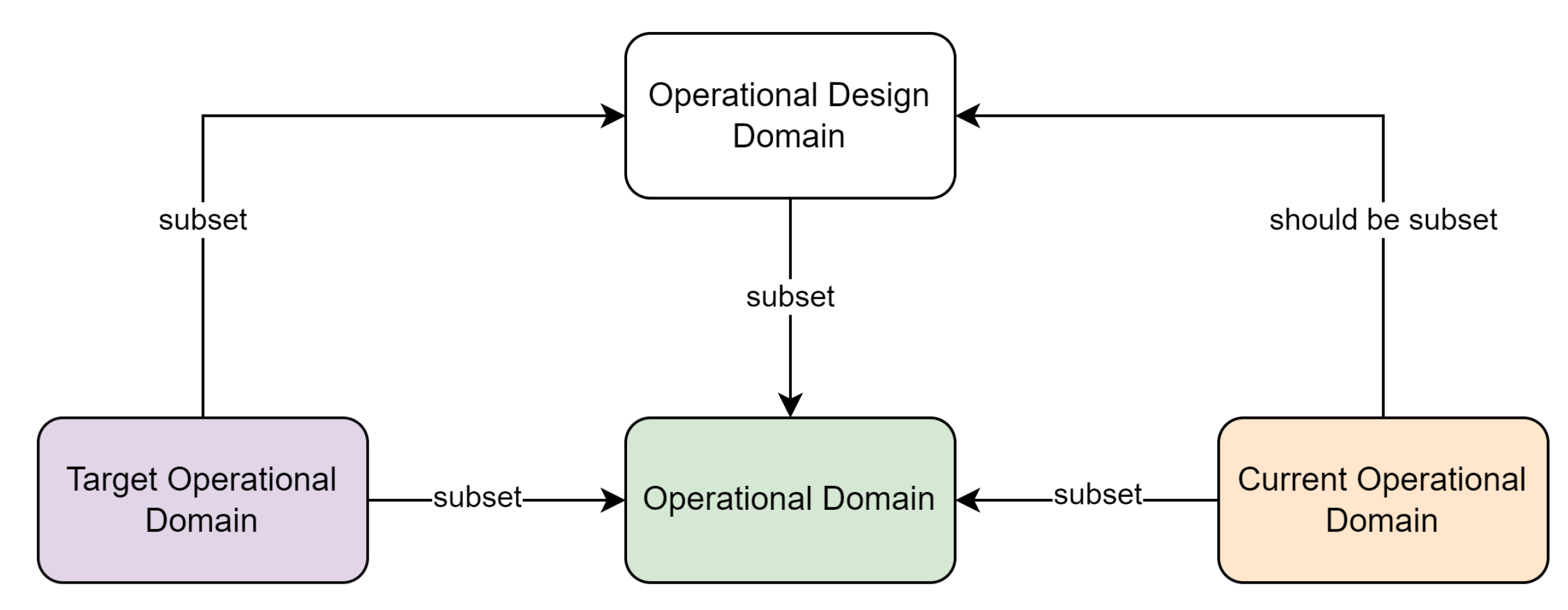
Figure 1. Relationship between OD, ODD, COD and TOD.
Preprints 113849 g001
Figure 2. ODD exits from perspective of SOTIF and ISO 34503.
Preprints 113849 g002
Figure 3. A workflow from creation of ODD to definition of OMS framework.
Preprints 113849 g003
Figure 4. Flow of road patch extraction for image classification.
Preprints 113849 g004
Figure 5. Summary of the RCE study.
Preprints 113849 g005
Figure 6. Class imbalance, number of images and accuracies in RCE over the years.
Preprints 113849 g006
Figure 7. Examples from the datasets.
Preprints 113849 g007
Table 1. Few significant works on OMS.
Paper (Year) Attribute Monitoring theme
 [20] 2017 Scenery, Dynamic elements Location and behavioural-based hazard threshold calculation
 [21] 2018 Scenery, Dynamic elements Restricted Operational Domain
 [2] 2020 Scenery, Dynamic elements Mapping of ODD, COD and TOD
 [22] 2021 Scenery Monitoring ODD of laser-based localization algorithms
 [11] 2022 Scenery, Weather, Dynamic elements Speed calculation, digitization of traffic signs, and road defects detection
 [23] 2023 Scenery Road topology monitoring
 [28] 2023 Survey ODD scope, creation, verification and monitoring
 [29] 2023 Scenery Connected dependability cage monitoring of ADS
 [26] 2023 Perception algorithms DNN-based perception algortihms runtime monitoring analysis
 [27] 2023 Perception algorithms Reliability error estimation from mapping of sensor data and OCs
 [25] 2023 Perception algorithms Correlating input feature space with safety specifications using ML
 [24] 2024 Perception algorithms Causal approach to monitor perception and control modules in ADS
 [3] 2024 Scenery, Dynamic elements Lane detection system monitoring
Table 2. Commonly used evaluation metrics for RCE.
Purpose Evaluation metric Definition Formula
Image classification Accuracy Ratio of correctly predicted instances over total number of instances. Acc. = T P + T N T P + T N + F P + F N
Precision Ratio of true positive predictions over all positive predictions P = T P T P + F P
Recall Ratio of true positive predictions over all positive instances R = T P T P + F N
F1-Score Harmonic mean of precision and recall F1 = 2 * T P 2 * T P + F P + F N
Average precision Sum of products of P and difference in R steps at each threshold AP = n ( R n R n 1 ) P n
Average precision at 50 AP value when IoU is greater than 0.50 AP50 = AP, when IoU ≥ 0.50
Mean average precision Mean of APs over all classes mAP = 1 C i = 1 C AP i
Semantic segmentation Mean Pixel Accuracy Ratio of correctly predicted pixels over total number of pixels mPA = T P + T N T P + T N + F P + F N
Intersection over Union Ratio of area of IoU of predicted segment to the ground truth I o U i = T P i T P i + F P i + F N i
Mean Intersection over Union Mean of IoU for all classes mIoU = 1 C i = 1 C IoU i
Regression Mean absolute error Average of all absolute errors MAE = i = 1 D | y i y ^ i |
TP: True Positives; FP: False Positives; TN: True Negatives; FN: False Negatives; C = No. of classes; D = No. of data points.
Table 3. Main classes and actually mentioned classes.
Main class Mentioned class
Dry Dry, Bare, None
Wet Wet
Water Water
Partially snow Partly snow covered, Drivable path, Standard, Slush, Melted snow
Full snow Snow, Covered, Fully snow covered, non-drivable path, Heavy, Fresh fallen snow
Ice Icy
Black ice Black ice
Tracks Tracks
Others Not recognizable, Others, Road materials
Table 4. Comparison of different RCE algorithms.
Paper (Year) Network Dataset Evaluation metric Result
No. of images No. of classes
[40] 1998 Feature extraction and simple NN 69 5: Dry, Wet, Tracks, Snow, Icy Acc. 0.52
[46] 2010 SVM 516 3: Bare, covered, tracks Acc. 0.85
[35] 2018 ResNet50 19000 6: Asphalt, dirt, grass, wet asphalt, cobblestone, snow Acc. 0.92
[33]3 2018 Custom CNN 5300 4: Dry asphalt, Wet/Water, Slush, Snow/Ice Acc. 0.97
[72]1 2019 D-UNet 2080 7: Background, dry, wet, snow, ice, water, tracks mIoU 0.79
[50] 2019 ResNet50 54,808 4: Bare, partly snow covered, fully snow covered, not recognizable Acc. 0.96
[49] 2019 Custom CNN and ReLu 10,000 5: Dry, wet, snow, mud, other Acc. 0.95
[89] 2020 Custom CNN 11000 4: Road, Wet road, Snow road, Black ice Acc. 0.98
[54] 2020 Custom CNN 1200 2: Dry, wet Acc. 0.92
[53] 2020 Custom CNN: TLDKNet 1000 3: Great resistance, medium resistance, weak resistance Acc. 0.80
[43]1 2020 ICNet 1075 11 mIoU 0.66
[83] 2021 CNN fusion 1000 2: drivable and non-drivable path mIoU 0.87
[55] 2021 RCNet 20757 5: Curvy, dry, icy, rough and wet Acc. 1.0
[38] 2021 Custom CNN 4244 4: Snowy, icy, wet, slushy F1-Score 0.92
[56] 2022 ResNet18 15000 3: Dry, snowy, wet/slushy Acc. 0.99
[58] 2022 ResNet50 18835 3: Dry, wet, icy; Time: day, night Acc, 0.98
[59] 2022 DenseNet121 45,200 3: Dry, wet, snowy Acc. 0.94
[41] 2022 MobileNetV2 720,000 12: RoadSAW F1-Score 0.64
[18] 20222, 3 ResNet50+ 5061 6: dry, wet, partly snow, melted snow, fully packed snow, and slush Acc. 0.87
[12] 2023 RF 21,375 3: Snow=None, standard, heavy Acc. 0.96
]2*[65] 2023 MobileNetV2 90,759 3: fresh fallen snow, fully packed snow, partially covered snow F1-Score 0.97
810,759 15: RoadSAW/RoadSC F1-Score 0.71
[80]1 2023 Mask R-CNN 800 Black ice AP50 0.93
[63] 2023 ViT-B/16 2498 8: Clear, Sunny, Cloudy, Wet, Snowy, Rainy, Foggy, Icy Acc. 0.92
[30] 2023 EfficientNet-B0+ 1 mill. 27: RSCD Acc. 0.98
[67] 2023 Attention-RexNet 1 mill. 27: RSCD Acc. 0.88
[85] ShuffleNetV2 8000 8 Acc. 0.98
[84]2 2023 Recurrent U-Net 1500 Drivable tracks Acc. 0.89
[44] 2023 2 Custom CNN 1000 2: drivable and non-drivable region mIoU 0.89
[68] 2024 EdgeFusionViT 1 mill. 27: RSCD Acc. 0.90
[15] 20243 Custom CNN: WCamNet 48791 Friction factors MAE 0.15
[95] 2024 Custom, SIWNet 4330; SeeingThroughFog (cite) Friction factors Average internal score 0.48
[14] 2024 CNN Meteoroligcal Fusion 600 5: Dry, fresh snow, transparent ice, granular snow, mixed ice Average precision 0.78
[45]3 2024 EfficientNet-B0+ 1 mill. RSCD Acc. 0.95
1: Semantic segmentation; 2: Drivable area detection; 3: Friction coefficient estimation.
Table 5. Factual comparison of two datasets.
Parameters RSCD RoadSAW/RoadSC
Number of images 10,30,000 810,759
Classes 27 15
Road material type Asphalt, Concrete, Mud, Gravel Asphalt, Cobblestone, Concrete
Wetness Conditions Dry, wet, water Dry, damp, wet, very wet
Winter Conditions Fresh snow, melted snow, ice Fresh fallen snow, fully packed snow, partially covered snow
Unevenness Smooth, slight uneven, severe uneven None
Class imbalance Yes No
Image/Patch size 360 * 240 px 2.56 m2, 7.84 m2, 12.96 m2
Patch distance from camera 10 m 7.5 m, 15 m, 22.5 m, 30 m
Image calibration None To Bird eye view
Annotation Manual Wetness: MARWIS, Snow: Manual
Maximum metric Acc: 89.76% F1-Score: 70.92%
Generalization analysis Confidence estimation from multiple overlapping images Deterministic Uncertainty Quantification, CtD datasets implementation
Velocity measurements No Yes
Disclaimer/Publisher’s Note: The statements, opinions and data contained in all publications are solely those of the individual author(s) and contributor(s) and not of MDPI and/or the editor(s). MDPI and/or the editor(s) disclaim responsibility for any injury to people or property resulting from any ideas, methods, instructions or products referred to in the content.
Copyright: This open access article is published under a Creative Commons CC BY 4.0 license, which permit the free download, distribution, and reuse, provided that the author and preprint are cited in any reuse.
Prerpints.org logo

Preprints.org is a free preprint server supported by MDPI in Basel, Switzerland.

Subscribe

© 2024 MDPI (Basel, Switzerland) unless otherwise stated