
Submitted:
01 August 2024
Posted:
02 August 2024
Read the latest preprint version here
Abstract
Unhealthy concentrations of ozone in the Uinta Basin, Utah, can occur after sufficient snowfall and a strong atmospheric anticyclone creates a persistent cold pool that traps atmospheric ozone and its precursors emitted from oil and gas operations. The winter-ozone system has two clear outcomes—occurrence or not—that is well understood by domain experts and supported by archives of atmospheric observations. Rules of the system can be formulated in natural language (“sufficient snowfall and high pressure leads to high ozone"), lending itself to analysis with a fuzzy-logic inference system. This method encodes human expertise as machine intelligence in a more constrained manner than alternative, more complex inference methods such as neural networks, increasing user trustworthiness of our model prototype before further optimization. Herein, we develop an ozone-forecasting system, Clyfar, based on knowledge of system dynamics and informed by an archive of meteorological conditions and ozone concentration. The inference system demonstrates proof-of-concept despite rudimentary tuning. We describe our framework for predicting future ozone concentrations if input values are drawn from numerical weather prediction forecasts as a proxy for observations as the system’s initial conditions. Our model is computationally cheap, allowing us to sample uncertainty with substantially more ensemble members than in traditional NWP. We evaluate hindcasts for one winter, finding our prototype demonstrates promise to deliver useful guidance for users concurrent with optimization of system parameters using machine learning.
Keywords:
fuzzy logic
; machine intelligence
; ozone
; forecasting
; air quality
; meteorology
; decision-making
1. Introduction
High, unhealthy concentrations of ozone in the Uinta Basin, Utah [1] (Figure 1) within the U.S. Intermountain West can occur after sufficient snowfall and a strong atmospheric anticyclone creates a persistent cold pool that traps atmospheric ozone and its precursors emitted from oil and gas operations [2,3,4]. While snowfall predictions are difficult due to sensitivity to temperature and altitude in mountain regions, the Uinta Basin winter-ozone (UBWO) physical system is well understood by domain experts, and future states become more predictable once the snow is present with an abrupt decrease of sensitivity to initial conditions. We conceptualize the system as falling into two possible states, or basins of attraction that represent cold pool formation: the development of ozone concentrations that exceed the U.S. Environmental Protection Agency (EPA) regulation, or not. Quantities such as snow depth, ozone concentration, and wind speed are continuous and subject to error, and rules of the system behavior can be described with adverbs of degree (e.g., “quite", “sufficient"). This scientific problem—modeling a well understood physical system with sparse, imperfect data—lends itself to a fuzzy-logic inference prediction system [5,6]. Fuzzy logic, an elemental form of machine intelligence, swaps familiar two-valued logic (True or False) for a continuum between those Boolean limits of zero and unity. We detail an early version of our prediction system herein.
The EPA regulates ozone concentration via National Ambient Air Quality Standards (NAAQS). We define a high-ozone episode when our representative observation for daily maximum ozone concentration in the Uinta Basin exceeds the 70-ppb NAAQS limit. We choose this threshold as multiple exceedances can trigger sanctions, leading to limits on and higher costs for industrial development. As such, forecasts of cold-pool and high-ozone events are critical to warn the oil and gas industry, protect public health, and support the regional economy. Since winter ozone only occurs during relatively rare and particular meteorological conditions, accurate predictions would allow decision-makers to reduce emissions when decisions are most crucial. The Ozone Alert system, run at the Bingham Research Center (BRC) in Vernal, Utah (Figure 1) since 2017, provides qualitative winter ozone forecasts to a network of over 100 oil and gas operators, other stakeholders, and local residents. The program was developed following a request by oil and gas companies; the regional oil and gas trade association encourages its members to participate, including distribution of mitigating steps to reduce emissions during winter ozone episodes. Thus we seek a guidance system to replace the current manually administrated email list.
However, traditional grid-point numerical weather-prediction (NWP) models struggle to capture both cold pools [3,7], snowfall [8], and high concentrations of ozone [9,10]. Further, approximations of sub-grid-scale processes can perform poorly in mountainous regions [11], hence forecast systems might be better developed specifically for mountainous application [12] given compounding errors in atmospheric chemistry and dynamical processes [13]. Observational data is relatively sparse in the Basin for radar and in-situ observations (not shown), posing an issue for training and/or evaluation of grid-based prediction systems. Any physical NWP model must resolve complex terrain to capture persistent cold pools in complex terrain; this is generally set as a horizontal grid-spacing finer than in NWP models. However, increasing the fineness of NWP grid-spacing in two or three spatial dimensions rapidly raises computational demand, considering the reduction in timestep to satisfy the Courant–Friedrichs–Lewy criterion (i.e., information does not cross more than one grid cell per timestep). The operation of developmental NWP forecasts locally (e.g., [14,15]) demands considerable resources and codebase development to ensure stability. Given finite computing resources, NWP running at finer resolution must come at the sacrifice of number of ensemble members, leading to our insufficient sampling the uncertainty of future states. This is despite more members being required to capture the finer-scale phenomena captured by a smaller truncation scale [16]. Wind flow across the Basin, a complex landscape carved with canyons and surrounded by mountain ranges, is subject to diurnal reversal of slope flows, channeling in the canyons, and other small-scale patterns that cannot be observed with the sparse network of observations in the Basin. While fine resolution is required to capture the mechanisms leading to cold pools and high ozone, the intricacy of streamlines across the Basin flow is an unknown unknown, yet a product of this high-resolution model. This appears irreconcilable for resolving a shallow planetary boundary layer such as a UBWO cold pool. What are our alternatives to this traditional configuration of NWP ensembles?
We might turn to a suitable form of artificial intelligence (AI), given many atmospheric scientists have employed state-of-the-art methods in AI suitable for operational forecasting (e.g., [17,18]), including those relevant to air-quality ([19,20], e.g.). Alternatives to traditional NWP can range in complexity from simpler statistical relationships [21] to pure deep-learning AI models [22,23,24]. Through the Information Age, AI and machine learning (data-focused) techniques have become more powerful and accessible through open-source software such as scikit-learn [25], PaLM [26,27], BLOOM [28], and so on. Many studies use artificial neural networks (ANNs) to capture patterns in data, sometimes leveraged to implement a forecasting system (e.g., [23,29,30,31,32]), other times to diagnose a system state (e.g., [33,34,35,36]). These ANNs represent an exhaustive set of permutations between input variables whose pathways activate beyond a critical value (in the hidden layer) to classify an output state. Further, Random Forests (RFs) also mimic human logic via a group of decision trees [37]. While powerful models have never been more accessible, the pitfall is black-box behavior where the human supervisor cannot fully trust generated output because they are not sure how the conclusion was reached [38]. Herein, we seek the simplest model that gives useful guidance, and no simpler; at this point, developers may use post-processing or deep learning to fine-tune model performance by optimizing parameters [39,40]. We must consider how to map our continuous variables (e.g., snow depth, ozone concentration) to degrees of a concept used by domain experts articulated in natural-language rulesets, such as “background ozone" and “sufficient snow". Our prediction can be considered inference from a dataset whose structure is described in natural, fuzzy language [41].
We develop herein a prototype ozone-concentration prediction system for the UBWO system, named Clyfar, which implements a fuzzy-logic inference system (FIS) that infers the possibility of a cold pool from meteorological input with rules drawn from human expertise and archived observations. While outside the scope of the present manuscript, the upcoming first version of Clyfar will ingest pre-process NWP forecasts as a proxy to current observations, and this generates ozone-concentration forecasts in the form of a “best guess" scalar value, in addition to a level of possibility (likelihood) of categories representing ozone levels (“background", “extreme", etc). We plan deployment as follows, where points 1–3 are described herein:
- Through domain knowledge, identify key input variables (snow, pressure, etc.) along with the output variable (maximum daily ozone concentration),
- Configure the FIS with behavior described in natural language by domain experts,
- Test the FIS performance in real-world situations to determine ability to capture high-ozone events,
- Use representative forecast values derived from NWP as input variables as a proxy for observations,
- Evaluate performance to advise optimization of parameters such as membership functions, rulesets, and choice of variables.
Following a description of data collection in Section 2, we provide more background for fuzzy logic in Section 3—a topic perhaps unfamiliar to readers. Next, we follow with rationale behind the configuration of Clyfar in Section 4. We present results from synthetic, illustrative forecasts in Section 5 and present a case study in Section 6 that used initial conditions from 2022 UBWO data to issue a hindcast we can compare to the observed ozone concentration values. We synthesize the performance and interpretation of Clyfar in Section 7 in the light of the team’s imminent goal to deploy Clyfar for operations and later evaluation. We then conclude and lay out a framework for building on Clyfar and other future work.
2. Data
We define these terms for the benefit of the reader unfamiliar with meteorological forecasting:
- An ensemble
- is a Monte Carlo simulation, here either NWP input or Clyfar members each driven by observations or forecasts. Ensembles are used to estimate a probability distribution of possible future states.
- Deterministic forecasts
- in the weather-forecasting sense are those with a scalar value, often produced from an average in the case of generating a time series of ozone concentration. This is opposed to probabilistic forecasts from an ensemble.
2.1. Engineering Representative Observations
We obtained atmospheric measurements from the compilation of sensor networks archived by Synoptic Weather (www.synopticdata.com, accessed 1 July 2024), a spin-off from MesoWest [42]). The geographical domain is a 72-km (45-mile) radius around Pelican Lake (UCL21) with coordinates (40.1742, -109.6666), shown by the red circle in Figure 1. This was chosen to best capture the Basin and surrounding high terrain. We target prediction of daily ozone-concentration maximum, defined in the local time-zone period of midnight to midnight. Observation stations can have different suites of atmospheric sensors, and use of one station leaves the analysis susceptible to spurious error. We therefore use the following functions to reduce observation sets to a Basin representative value configured after extensive preliminary testing and discussion between domain experts:
- Snow-cover data are sparse in the Basin (stations reporting snow depth are marked with black squares in Figure 1), where most stations at Basin level are operated by via volunteers in the Cooperative Observation Program (COOP; https://www.ncei.noaa.gov/products/land-based-station/cooperative-observer-network, access 1 July 2024). A station that reports once a day may not sample at a time most representative for that solar day. Therefore, our snow value is the 90th percentile of the set of maximum snow-depth reports from Basin-floor stations on the COOP network taken at minimum once a day.
- Raw pressure data is reduced to mean sea-level pressure (MSLP) on Synoptic Weather’s server before download, and we use the median value from all stations’ daily maximum as representative. The computation of MSLP becomes less reliable with height, and preliminary work revealed absolute values of MSLP in the dataset to be excessively large. The excessive MSLP values appear to be a systematic, additive offset that does not preclude good performance (not shown). Current work is investigating alternative calculations of MSLP and the source of high bias.
- Insolation is affected by both optical depth (humidity and clouds; particulate matter) and the solar angle. Passing clouds make the data temporally variable, and spatially, higher elevation stations will receive more radiation under clear skies. To generate a representative value for the Basin, we employ a “near-zenith mean" that takes the mean downwelling solar radiation for each station between 1000 and 1400 local time. From this set of all stations, we then take the median value.
- Wind data. We want to capture wind strong enough to disperse pollutants and/or the cold pool, while ignoring transient gusts from storms (mainly a result of evaporative cooling and attendant downdrafts). Hence, we assume Vernal Regional Airport (KVEL) is representative and take its daily median 10-meter maximum reported wind value, with the benefit of a long, reliable archive of observations. The airport is approximately 4.5 km (2.8 miles) from the nearest foothills east of the runway, and even further from canyon exits north of the town. As such, we neglect effects from downslope winds, drainage flows, or wind funneling; we take KVEL wind reports as representative of the Basin as a whole.
- Ozone data. While internal data shows there is occasionally considerable variation in ozone concentrations from west to east in the Basin (not shown), for the purpose of this initial study we choose one value by taking the 99th percentile of each station then take the median value from this set.
3. Fuzzy Logic: Background and Justification
Fuzzy logic differs from traditional two-valued logic (True or False) by allowing variables to have continuous set membership between 0 and 1. For example, if a person is of average height, we may say in fuzzy language that they are 0.5 tall and 0.5 short. This is a more intuitive mathematical concept than forcing a binary choice of entirely “tall" or “not tall". Likewise, we can encode nuance in our ruleset by having a gradient between clusters or categories within a given variable. We can use domain expertise to determine numerical values for adjectives using when creating a ruleset for the system at hand. The use of fuzzy logic is motivated by multiple characteristics of the system:
- The formation of UBWO cold pools
- —and hence high ozone concentration—is a well known system, but hinges on sufficient snowfall. As a complex system with two basins of attraction, sensitivity of cold-pool formation is lower when snow is either absent or very deep, whereas near the cusp of the two potential future states (near the bifurcation point), chaotic growth means small changes grow rapidly [43,44]. Setting a single representative value for snow depth is difficult due to drifting, sparse data observations, and inherent limitations of human knowledge and ability to represent UBWO system complexity. Fuzzy logic effectively smoothes a portion of uncertainty, and is resilient in presence of error [45], trading some specificity for the estimate of uncertainty.
- The need to deliver forecasts in different manners for stakeholder needs:
- both a deterministic manner (i.e., a scalar value or best guess of ozone concentration in native units) and one that conveys risk (i.e., a risk, such as 20%). The former is sharper, more specific, but more susceptible to “catastrophic error" [46] for risk-averse users; the latter is more complex to communicate but enables decision-making under uncertainty appropriate for user vulnerability [47] and extends the time horizon to which we have predictive utility [48].
- Data sparsity
- makes it difficult to evaluate the fidelity of a fine-gridded O(1 km) NWP model, and the difficulty to finding a representative numerical value means encoding human knowledge with flexible natural language.
- Evolution of an AI system with ongoing development and optimization
- that can be increased in complexity to optimize output utility to Ozone Alert forecasters and decision makers.
- Capturing both complex terrain and uncertainty
- is a trade-off when running expensive NWP models. As grid spacing becomes finer, timesteps between integrations must become closer together, and we might consider a finer grid in the vertical direction to better capture shallow cold pools in simulations. However, a rare event (e.g., a heavy snowfall that occurs 1 in 5 winters) requires ample sampling of the uncertainty distribution. The fewer members in a forecast ensemble, the less chance of capturing the true nature of uncertainty, and the more difficult to calibrate the system to optimize balance between sharpness and reliability of uncertainty estimates. Further, fine-scale atmospheric flow and state is an unknown unknown: a high-resolution NWP model may waste its resources in a similar way as upscaling (e.g., doubling the pixel count of) a blurred photograph is a worthless task. However, we lack the observations to diagnose such a scenario: the so-called curse of dimensionality.
As such, we seek an alternative that eschews NWP for a simpler rule-based system, and based on representative input values processed from the limited observations available in the Basin. We can model the UBWO system with fuzzy logic, whereby concepts important to the system—such as “sufficient snow"—are first identified in observed data and then quantified. For instance, if the domain expert orates that “high ozone“ typically follows “snowfall exceeding around 4 inches`, this can be codified as snow ⪆100 mm leading to ⪆70 ppb. The remaining subjective element of how to quantify “approximately" for both values is addressed with a membership function. If a deep snowpack is required for ozone production, a snow depth of 25 mm (1 inch) is clearly not “deep" and may be considered in fuzzy logic as 0.8 “negligible" and 0.2 “sufficient" as its nature as a necessary condition for UBWO high-ozone events. This is a fuzzy set, in contrast to the bivalent logic or two-valued sets familiar to most readers: in that paradigm, snow is, or it is not, sufficient for high ozone values.
We are also motivated to use a FIS to follow best practices of explainable AI [38]). The concept of trustworthy AI is sensible: if a colleague were wrong a finite number of times per week, you would not let them make executive decisions without supervision. A FIS encodes domain knowledge explicitly, enabling explainable and transparent construction of its workings and can be extended with a fuzzy neural network (e.g., [49]) or fine-tuned with deep-learning (e.g., [50]). Herein, we create a prototype model to demonstrate potential of forecasting ozone concentrations for the purpose of automation, optimization, and greater insight into UBWO-system behavior. Comprehensive reviews of fuzzy logic can be found in, e.g., [51]. We perform inference with the so-called Mamdani method, which the authors found more accessible; further information on alternatives, such as the Sugeno method, is outside the scope of this manuscript.
4. Configuration of Clyfar
We define membership functions for each category in each variable informed by an archive of meteorological and ozone-concentration observations. Though the authors had access to 20 years of data for this region, the present study will focus on the winter of 2021/2022 as suitable to demonstrate the promising, but mixed, results of our prototype. To simplify our prototype for sake of understanding, we restrict our system to four input weather variables with ozone as the sole output variable.
4.1. Overview of Approach
Some users seek a deterministic forecast, perhaps interpreted as a best guess. However, others benefit from information about uncertainty, increasing the chances of detecting an early, low-risk, high-impact event [52,53] by accounting for chaotic error growth [43,48]. Inference of both an output value and uncertainty distribution follows this method:
- Pre-process observational data to create a representative value of the Basin state per input variable. This process is also known as feature engineering. In future, these numbers can be replaced with forecast values from national NWP models;
- Define Linguistic Variables: Identify and define the variables with linguistic categories (e.g., negligible or sufficient snow depth)
- Create Membership Functions: Define membership functions for each linguistic variable. These functions map the input data to their corresponding fuzzy sets, representing modifiers (“adverbs of degree"),
- Construct Fuzzy Rules: Develop a set of if–then rules that define the relationship between input and output variables based on domain expertise (e.g., "Sufficient snow and calm winds lead to high ozone.")
- Fuzzification: Convert the crisp input values into fuzzy values using the defined membership functions. For example, shallow snow mm (1 inch) deep might become “negligible" and “sufficient".
- Apply Inference Rules: For each fuzzy rule, we compute an activation of the target variable’s category. Rules use fuzzy operators: (AND) from two-valued logic is formed as , while (OR) becomes ;
- Defuzzification: Convert the fuzzy output values back into crisp values using defuzzification methods such as the centroid method (a sort of weighted average). This generates a single, deterministic value in native units.
We refer to our fuzzy-logic prediction system as Clyfar. This is Welsh for "clever" to reflect our focus of codifying human expertise as machine intelligence, and is a loose abbreviation of "Computational Logic Yielding Forecasts for Atmospheric Research". To gauge performance of Clyfar, we feed crisp values to compare forecasts to observed ozone concentrations. Our system is assumed stationary, as therefore the model should capture the UBWO key behavior with observations before forecasts can be issued. As there is no machine learning occurring at this stage of the FIS, there is no concern in training and testing over the same dataset. In a similar manner to humans’ ability to account for missing data in natural language, knowledge of the UBWO system characteristics is drawn from previous events for use in inference rules. Part of the benefit in generating a distribution of possibility levels from these fuzzy rules is bounding uncertainty [45,47] rather than estimating a crisp probability—the latter itself subject to uncertainty! Moreover, possibilities do not need to sum to unity, as with probabilities; further mathematical discussion is found in [45,56,57].
This inference system comprises multiple modules discussed in the coming section:
- Input pre-processing:
- so NWP forecasts or observed values of pertinent meteorological variables are reduced to a single input value through feature engineering to produce a representative value for the UBWO system initial state;
- The inference system’s ruleset:
- to generate an aggregated distribution of possibility (likelihood) for a range of daily maximum ozone concentration values;
- Two sorts of output:
- a deterministic prediction of ozone, generated by reducing the aggregation; and a forecast distribution that preserves the uncertainty information. Future versions of Clyfar will pass this output to further post-processing.
4.2. Input Pre-Processing and Membership Functions
Input variables were chosen by inspecting our archive of observations. Clusters or bifurcations in scatter plots of daily representative values of ozone concentration against various input variables, as shown for wind speed in Figure 2, represent potential regimes or areas of nonlinear behavior in the UBWO atmospheric state known to domain experts. For instance, Figure 2 shows that even a moderate wind speed can disperse the pollution and lower concentrations. In the following figures, the x-axis represents the possible range considered by the inference system (also called the universe of discourse); values outside of either bound are clipped to the appropriate minimum or maximum.
For demonstration and testing of our prototype—the ruleset becomes complex quickly as new input variables are added—we choose four inputs and one output. Let us assume each value is a representative value for the Basin as a whole. We choose the follow input variables that will result in some sort of ozone forecast:
Figure 2.
Scatter plot of representative ozone against wind speed for the 2021–2022 winter. The purple dashed line indicates the NAAQS limit. Red scatter markers denote days in exceedence of the NAAQS limit; orange markers are within 10 ppb.
Figure 2.
Scatter plot of representative ozone against wind speed for the 2021–2022 winter. The purple dashed line indicates the NAAQS limit. Red scatter markers denote days in exceedence of the NAAQS limit; orange markers are within 10 ppb.
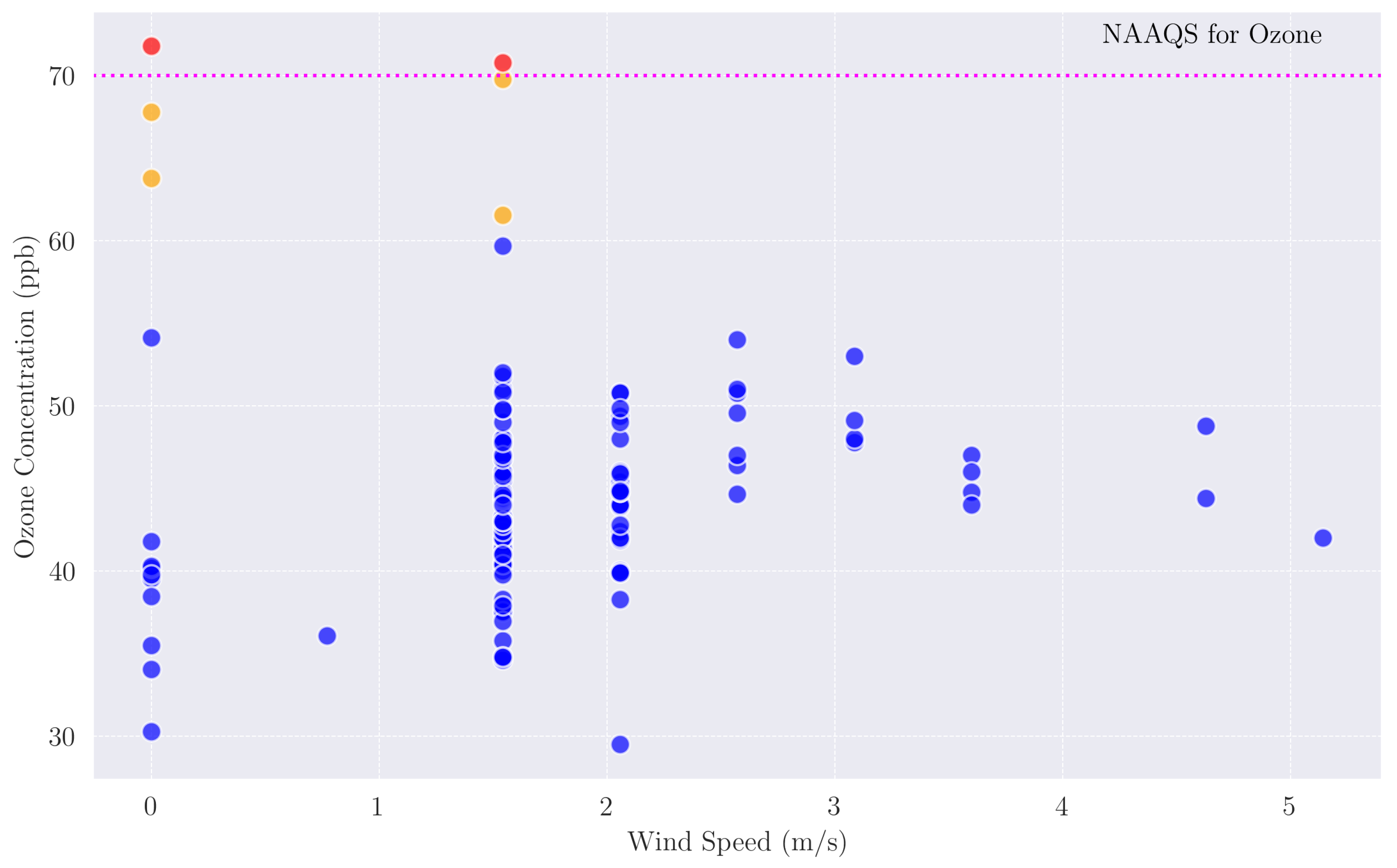
Figure 3.
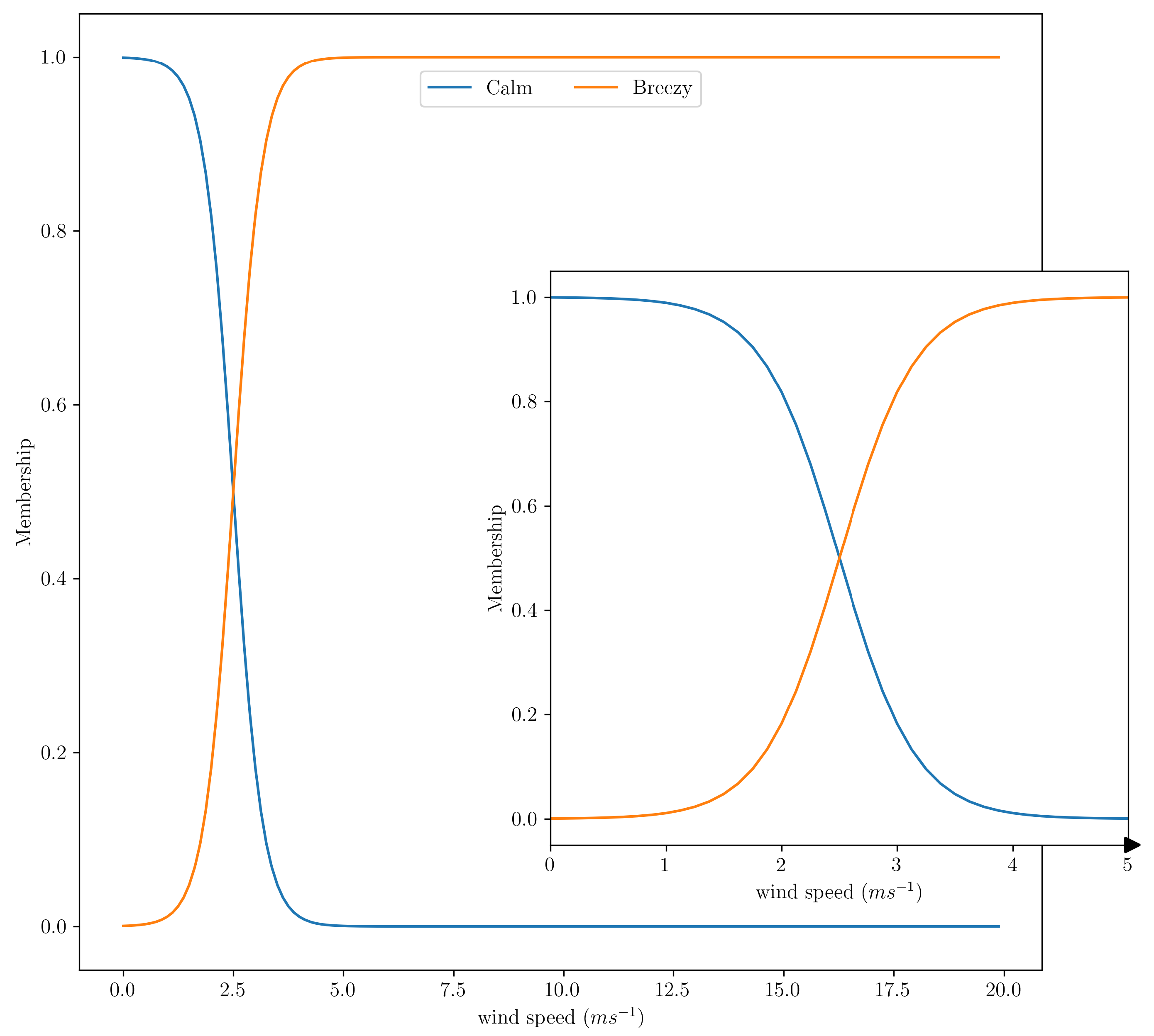
Membership function for daily 90th percentile of 10-m wind speed. Inset shows zoom highlighting the function shape around where the two cross.
Figure 3.
Membership function for daily 90th percentile of 10-m wind speed. Inset shows zoom highlighting the function shape around where the two cross.
- Snow depth.
- As seen in Figure 2, exceedence events in winter 2021–2022 only occurred if the representative wind was calm enough. Preliminary testing showed this was common to numerous stations and seasons, matching domain expertise. We chose two opposing sigmoid distributions crossing close to 2.5 as advised by observations and adjusted slightly during preliminary testing.
- Wind speed.
- Similarly to the wind variable, we choose two opposing sigmoid functions that cross around a region of “sufficient snow". This is around 100 mm (3.9 inch). Although difficult to directly compare, the sigmoid shapes were shallower resulting in more likely overlap when more frequently observed in the UBWO system (cf. the inset of Figure 4) to represent more uncertainty around what constitutes “sufficient" ozone.
- Mean sea-level pressure (MSLP).
- Rising pressure behind a snow storm reinforces the surface anticyclone in cold air, often in tandem with warm air advection aloft (e.g., [7]). We choose three categories: two extremes are conducive to dissipation or formation of cold pools, while the middle category essentially increases specificity (an additional membership function curve) at the cost of increasing the ruleset complexity. Regarding magnitudes of mean sea-level pressure (MSLP), values appear too high, perhaps due to calculation error, but preliminary testing showed no obvious errors. This will be adjusted in future. The authors also tested for sensitivity to normalization of input data (i.e., pressure in [0,1]) due to the large gap in ranges between MSLP and the other variables. There was no observed improvement in performance, with some loss of transparency due to the required transform to and from the normalized range [0,1].
- Solar insolation.
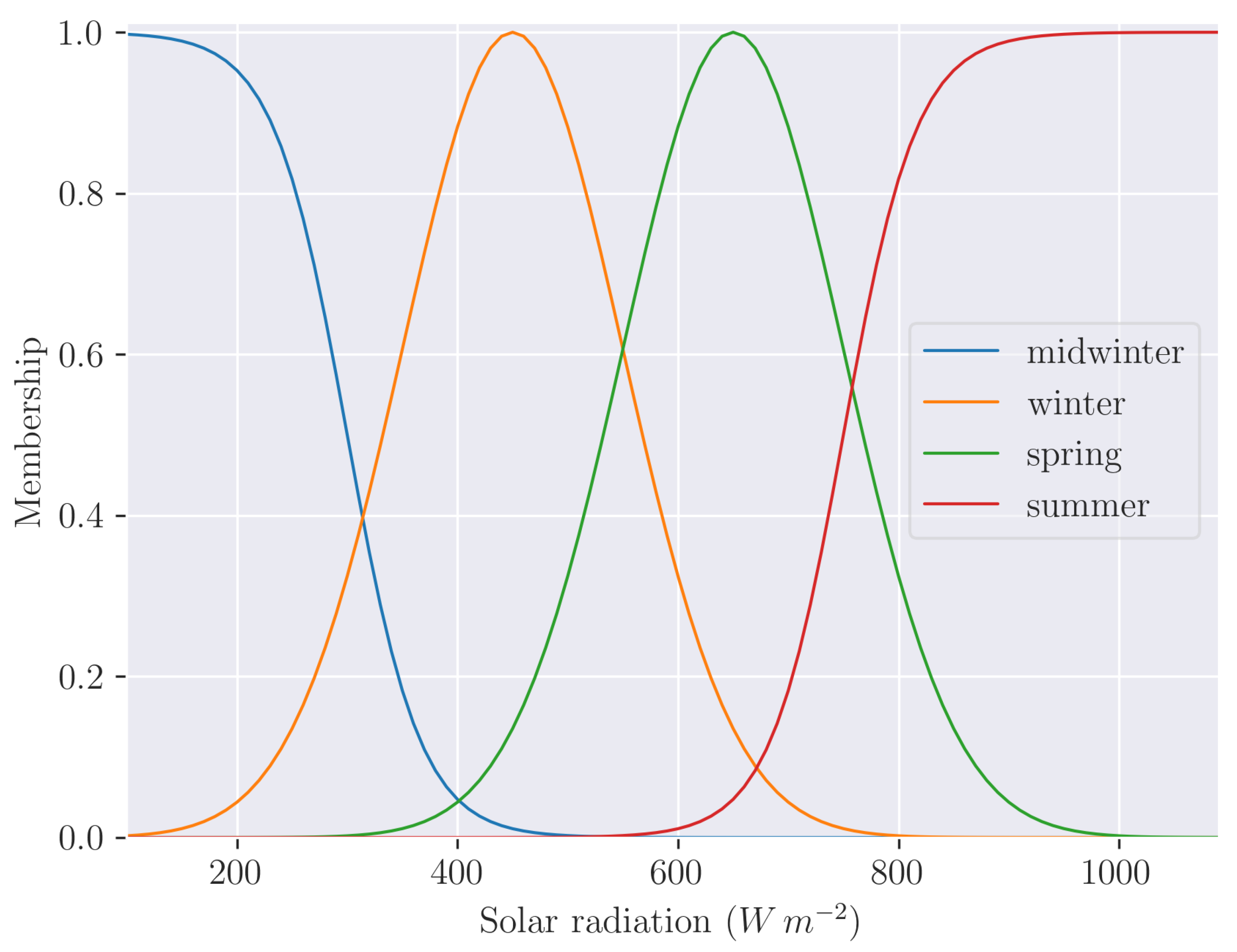
- The authors found most subjective uncertainty and sensitivity when considering downwelling solar radiation critical for photolysis and the process leading to unhealthy ozone concentrations. Solar insolation measured at the surface is highly sensitive to cloud cover factored nonlinearly by the time of day where solar obscuration occurred. The further complexity in the ozone–insolation relationship is how increasing insolation increases with photolysis and ozone production, but eventually mixes out the cold pool due to melting snow and thermal mixing of the planetary boundary layer. We encode this large uncertainty with larger overlap of membership functions (Figure 6). We decide to define four periods to reflect the four main months of the UBWO system (December to March inclusive) and parallel the ozone output categories discussed next.
Figure 4.
Membership function for daily median snow depth. Inset shows zoom highlighting the function shape around where the two cross.
Figure 4.
Membership function for daily median snow depth. Inset shows zoom highlighting the function shape around where the two cross.
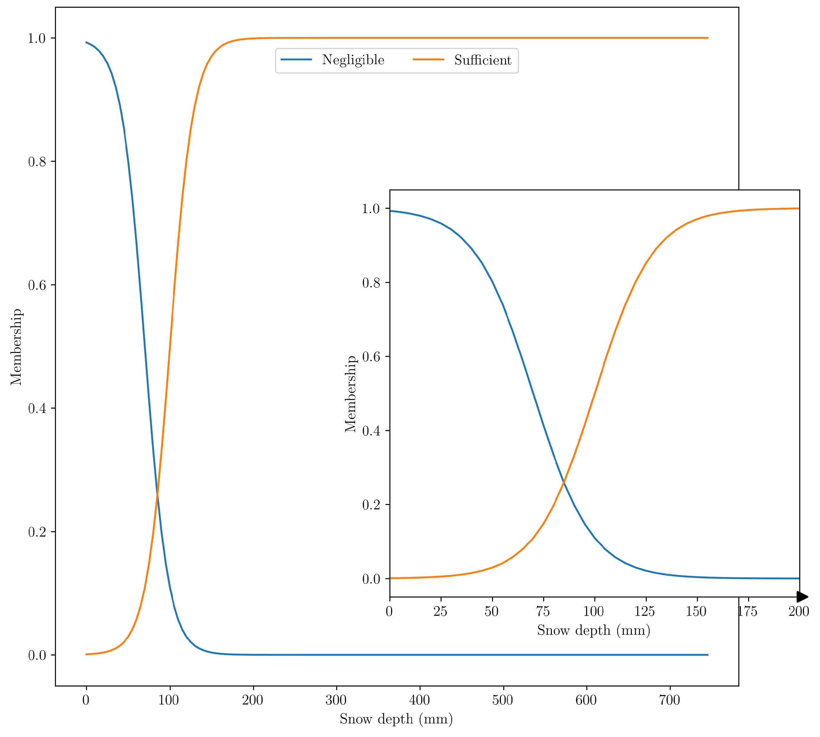
Figure 5.
Membership function for daily median mean-sea-level pressure (MSLP).
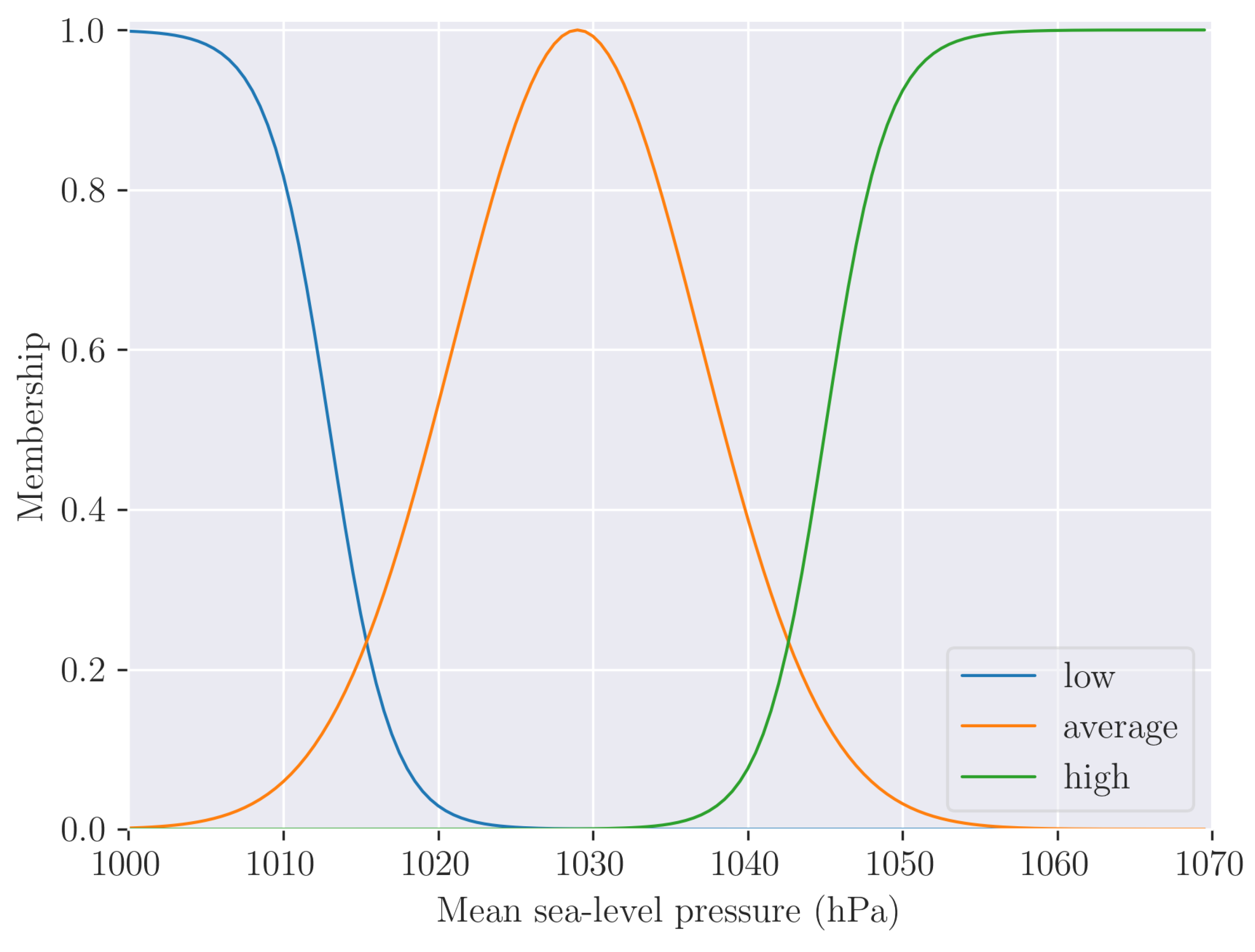
Figure 6.
Membership function for incoming short-wave solar radiation.
4.3. Output Products
The output is ozone concentration in four categories: background, moderate, elevated, and extreme. We choose not to match the categories currently used by the Uintah Basin 1 air quality (UBAIR) website (www.abair.usu.edu, accessed 1 June 2024) to focus on optimizing for the FIS without restriction on output-variable membership functions. The choice of four categories strikes a balance between complexity (required to capture extremes) and simplicity (to reduce the size of the FIS ruleset). Not all permutations of these rules are needed as they are either physically inconsistent (e.g., snow is sufficient and solar is summer) or already captured by another rule (optimizing the ruleset is outside the scope of the current text). Again, it is human expertise that can handpick or modify rules, adding trustworthy complexity. Next, we use relationships between input variables and ozone concentration samples to determine membership functions.
4.4. Mathematical Implementation
Each category per variable is described by a membership function, and corresponds to a distinct level of the variable; we tailor the functions to subjectively represent observed behavior. The membership functions are constructed using Gaussian or sigmoid functions. Gaussian curves are each defined by mean () and standard deviation () values. This approach is implemented with the scikit-fuzz Python module [58] (https://github.com/scikit-fuzzy/scikit-fuzzy, accessed 1 January 2024). The general formula for each ozone level’s membership function is given by:
where “level” is replaced by the descriptive term for each membership function. We also use sigmoid (“S-shaped") functions in the FIS mechanics to represent variables that asymptote to 0 or 1. The sigmoid membership function is generated with the equation
where is the membership value with respect to x; x is the variable of interest; b is the center value of the sigmoid (); c controls the width of the sigmoidal region about b (magnitude) and determines the function’s shape. A positive value of c implies the left side approaches 0.0 while the right side approaches 1.0; likewise, vice versa for a negative sign. We show numerical values for each variable category’s membership function in Table 1. Hereafter, we italicize variable categories (e.g., sufficient snow) to differentiate fuzzy-variable adverbs from body text.
4.5. Ruleset of UBWO Behavior
In natural language, we can describe the Winter Ozone System with the following rules. We define a limited list of key rules known to human experts below for pedagogical reasons, but clearly the list does not exhaust the permutations of all variables and categories:
- If there is little snow, or pressure is low, or wind is breezy, then the ozone level will be at background levels. This is because pollutants are blown away from the region of interest;
- If there is sufficient snow, and if pressure is high, and if wind is calm, and if the solar radiation is typical for spring, then the ozone level will be extreme (typical high-ozone case).
- If there is sufficient snow, and if pressure is high, and if wind is calm, and the solar radiation is typical for winter, then the ozone level will be elevated.
- If there is sufficient snow, and if pressure is high, and if wind is calm, and the solar radiation is low (midwinter) or high (summer), then the ozone level will be moderate.
- If there is sufficient snow, and if pressure is average, and if wind is calm, and the solar radiation is low to moderate (winter into spring), then the ozone level will be elevated.
- If there is sufficient snow, and if pressure is average, and if wind is calm, and the solar radiation is lowest (midwinter) or highest (late spring into summer), then ozone level will be moderate. This is because insolation is either too weak for prolific ozone generation, or so strong it may mix out the boundary layer.

Table 2.
Logical symbol reference.
| Description | Rendered |
| Implication (IF...THEN) | → |
| A AND B | A ∧ B |
| A OR B | A ∨ B |
| NOT A | ¬A |
We can construct rulesets for the ozone system as follows (mslp denoting MSLP):
5. Synthetic Examples
Here, we assess our system with synthetic examples to demonstrate expected behavior for four scenarios whereby unhealthy levels of ozone are deemed (1) likely, (2) unlikely, (3) on the cusp of occurring or not, and (4) an implausible scenario of snow in summer.
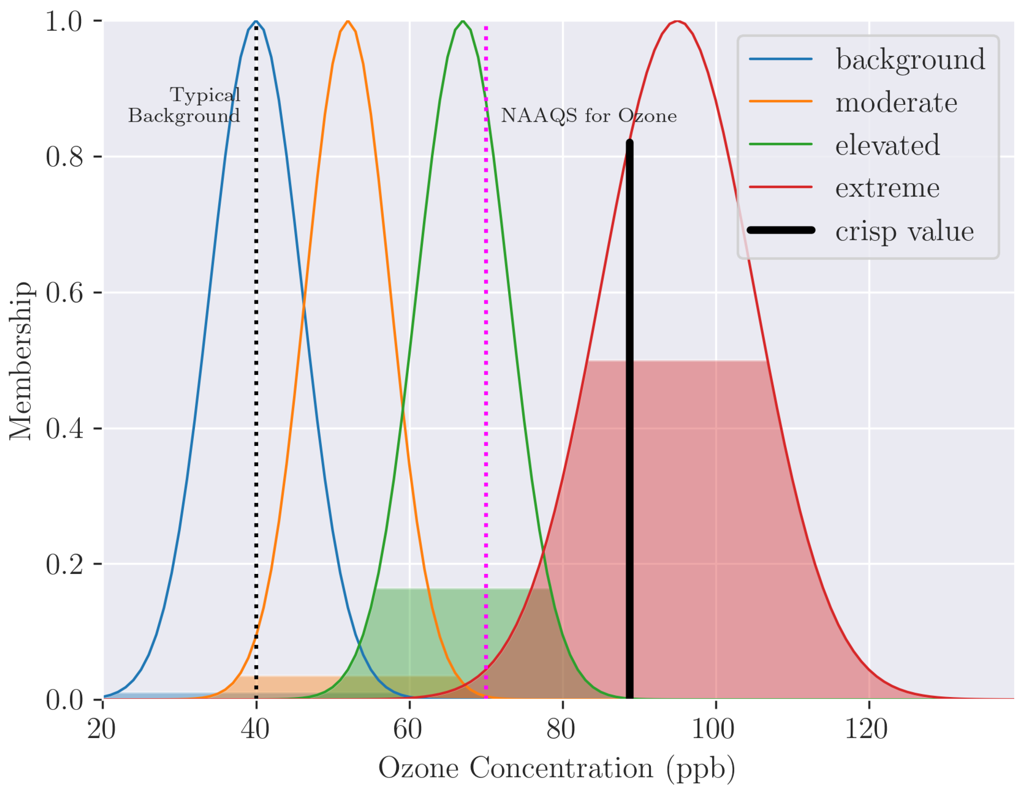
5.1. Case 1: Ozone Likely
We begin with an example in a situation where ozone levels are expected to be higher than the NAAQS limit, given deep snow, high pressure, weak winds, and insolation strong enough to instigate ample ozone production but weak enough not to mix out the cold pool.
- snow = 250 mm (9.8 inches)
- mslp = 1045 hPa
- wind = 1.0
- solar = 640
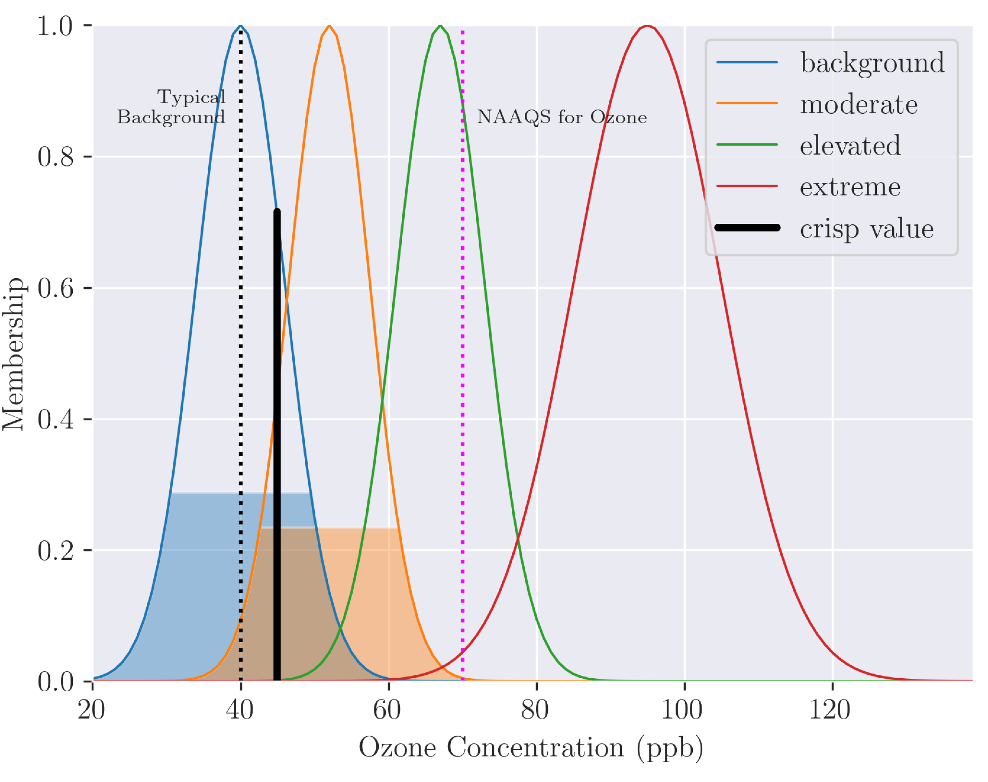
The crisp value predicts a ozone level of 75 ppb. Looking at the four categories, there is little support (possibility) of background and elevated levels of ozone, but strong possibility for extreme levels. The centroid method is used to generate a most-likely value, but by its nature of computing a weighted average over rule-activation aggregation, it cannot generate a crisp value to the right of the extreme Gaussian curve’s center value.
Figure 8.
The possibility of each ozone fuzzy set (filled color), membership function overlaid (colored line), both generated by the inference system for a likely high-ozone day.
Figure 8.
The possibility of each ozone fuzzy set (filled color), membership function overlaid (colored line), both generated by the inference system for a likely high-ozone day.
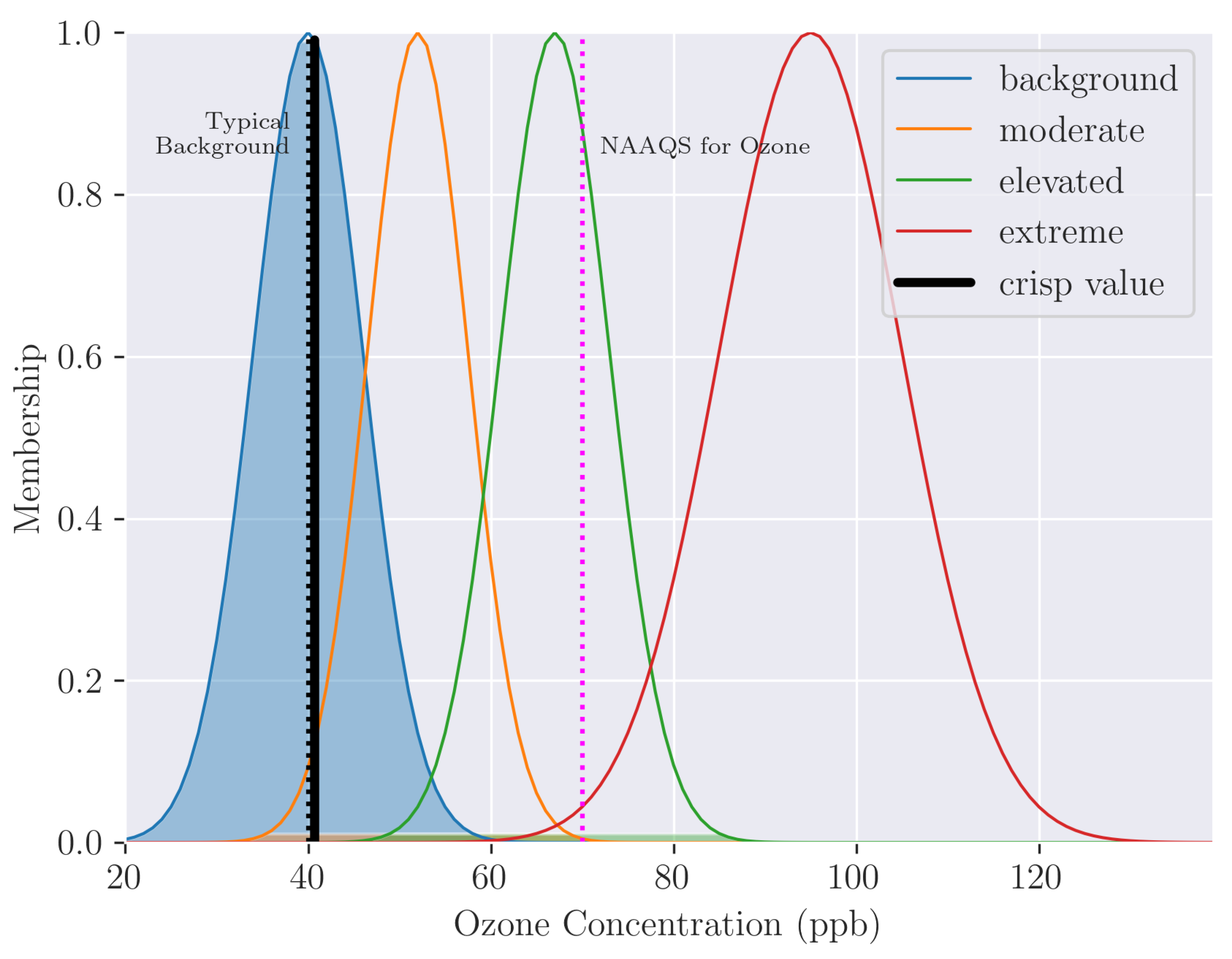
5.2. Case 2: Ozone Unlikely
Next, a case unlikely to yield ozone above a typical background level. We prescribe a thin snow depth and a breeze that would likely blow a portion of pollutants from the Basin and/or initiative mechanical mixing of the cold pool and dissipation into the free troposphere.
- snow = 50 mm (2.0 inches)
- mslp = 1025 hPa
- wind = 4.0
- solar = 600
The inferred ozone concentration suggests it is entirely possible (likely) to remain near background levels. The impossibility of another outcome other than background is triggered by Rule 1 (breezy wind → background ozone). We recall that possibilities across categories can sum to more than one, unlike probabilities. Hence, not only is the possibility (activation) of background close to 1.0, the possibility of other categories are equal or near zero. A background level is not only totally possible but entirely necessary due to the impossibility of all other outcomes. Further information on possibility and necessity—dual measures that represent bounds on uncertainty—is found in [45].
Figure 9.
As Figure 8, but for a scenario unlikely to yield ozone in excess of background levels.
Figure 9.
As Figure 8, but for a scenario unlikely to yield ozone in excess of background levels.
5.3. Case 3: On the Cusp
We consider a case where it is deliberately not immediately clear which ozone level is most possible due to variables on the cusp of the membership function’s intersection (i.e., close to a potential tipping point in the physical system, such as sufficient snow).
Figure 10.
As Figure 8, but for a scenario at the cusp of yielding predictions of elevated ozone levels.
Figure 10.
As Figure 8, but for a scenario at the cusp of yielding predictions of elevated ozone levels.
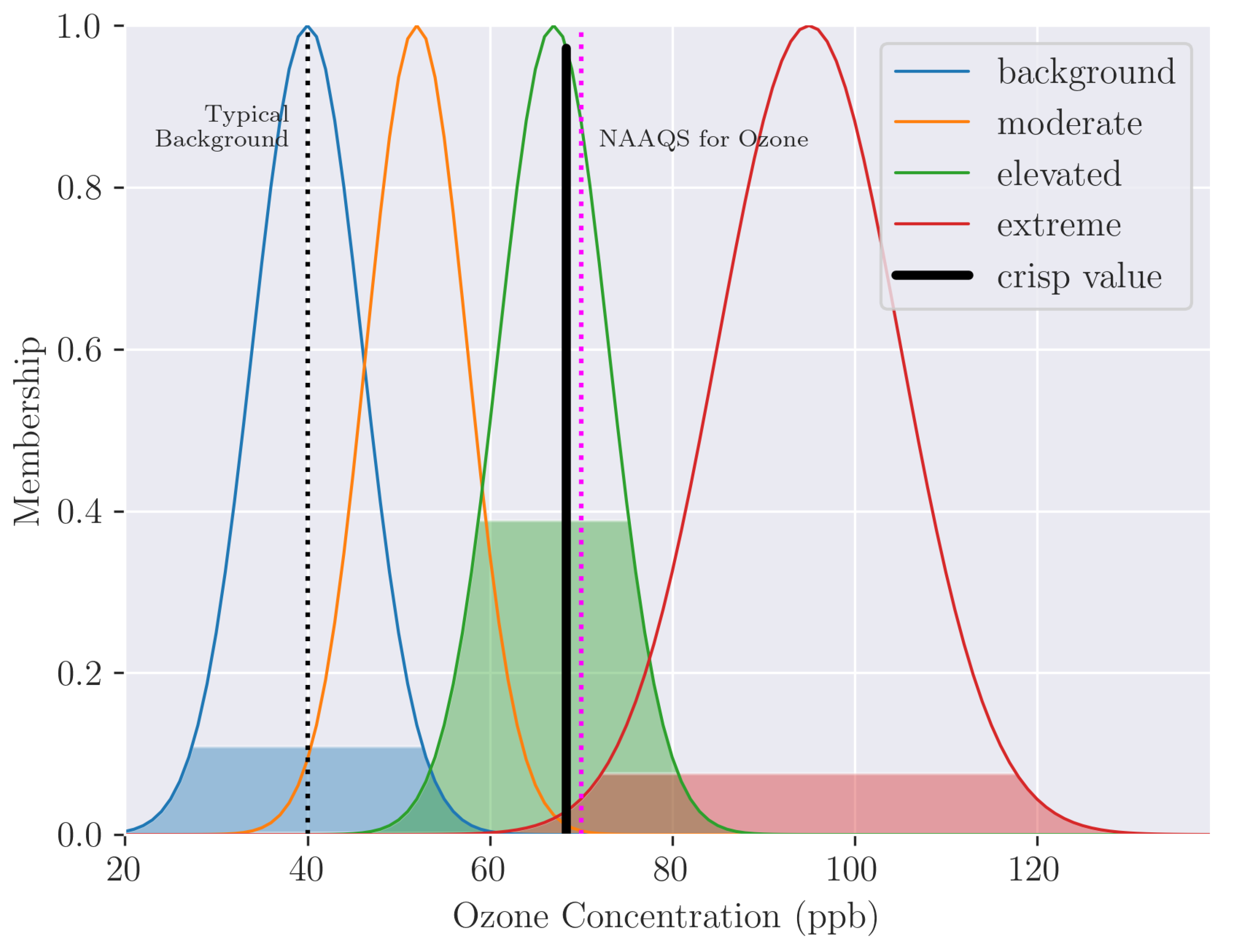
- snow = 100 mm (3.9 inches)
- mslp = 1040 hPa
- wind = 1.5
- solar = 500
The sum of all possibilities is less than unity: a so-called subnormal distribution [59]. While further discussion is outside the scope of this study, this signals insufficient rule coverage as something must happen (i.e., at least one category must be entirely possible before it may necessarily occur). Confirming a weakness in the ruleset construction, we find moderate was not activated but instead adjacent categories, which seems counterintuitive. Alternatively, this distribution and the two basins of attraction to ultimate states may indicate a bifurcation in solutions (i.e., it is difficult to discriminate between the two states).
There is a high possibility of elevated ozone, but there is also a considerable possibility of ozone limited to background levels. The activated range (filled area of membership functions in figures) around the crisp value (black line) is large, suggesting considerable uncertainty (i.e., a wide range of output variables are possible). In this case, a centroid value does not communicate the high uncertainty (i.e., the substantial possibility of other sets, particularly background). Further to this crisp (deterministic) value, stakeholders who are risk-averse would benefit from information that extreme levels are still possible in case evasive action makes financial sense (e.g., [60]).
5.4. Case 4: Ignorance
A common mantra for statistical processing states that “garbage in, garbage out"—unfortunately, “garbage out" and useful guidance are often indistinguishable before the event occurs or not. A supervising human in loop or an automatic quality control may prevent nonsensical values from Clyfar processing, but let us consider raw output in an implausible scenario of summer snow.
Figure 11.
As Figure 8, but for an impossible scenario with summer snow, unforeseen by Clyfar.
Figure 11.
As Figure 8, but for an impossible scenario with summer snow, unforeseen by Clyfar.
- snow = 83 mm (3.3 inches)
- mslp = 1050 hPa
- wind = 1.0
- solar = 1100
We know Clyfar cannot offer a useful prediction. The lack of support in the data and a near-uniform distribution of (not very) possible outcomes represents substantial ignorance, which may be preferable over a deterministic, crisp ozone concentration that is extricated from scarce information. These cases resemble black swans [61] in that they have not been considered due to their absence in observation records. In a stationary climate with a long record of observation, we can confidently say some events—such as snow on July 1 at the Basin floor—are impossible, or “off the attractor" in the paradigm of chaotic, complex systems [62]. While we find Clyfar does suggest all outcomes are not very plausible, which is true, a non-optimized or restrictive model will continue to suffer from these problems if the set of rule permutations is not explored sufficiently.
6. Results: Winter 2021/2022 Hindcasts
We now present hindcasts from this preliminary version of Clyfar, here marked as version 0.1 (v0.1), using observed weather variables and evaluating against collected ozone data for the same daily periods.
This winter was characterized by one ozone exceedence event at the turn of February/March. This was associated with typical precursors familiar to domain experts, such as calm wind and antecedent snowfall (not shown). We highlight three regions of the 2021/2022 season that illustrate the good, bad, and typical performance quality of the Clyfar prototype. We order these subsections in chronological order; each event is labeled with a black arrow above the axis in Figure 12.
6.1. 14 December 2021: Example of Background Signal
As noted above, crisp (determinstic) forecast values generated from Clyfar cannot exceed the center of the Gaussian curve for each category book-ending the universe of discourse (i.e., background and extreme ozone). This hard limit is an artifact of the defuzzification method (here the centroid method, a sort of weighted average), and can be addressed by changing this method [63], or perhaps post-processing with another algorithm or model. We configure Clyfar in a modular manner to allow for modification of algorithms or pre-/post-processing independently during optimization.
When we view output as the possibility of each category (Figure 13), Clyfar suggests background ozone levels are almost entirely possible (), in contrast to almost impossible occurrence of the other, higher concentrations. Similarly to Figure 9, the impossibility of other categories makes background levels necessary—not just possible. Despite a high possibility value for background levels, we find this value to still be in the lowest quartile of possibility for the season. This is sensible: all else equal, it is more possible to achieve typical, background levels of ozone than rare, extreme levels. However, further interpretation is needed whether percentiles rather than raw possibility values are more useful to signal a potential low-risk, high-impact event at long (less predictable) lead times (e.g., [64]).
6.2. 2 January 2022: Poor Forecast
In this event, Clyfar predicted that an elevated level of ozone was most possible, but without high support in the data (evidenced by the possibility value ).
We note that extreme levels of ozone, while deemed not likely by Clyfar, are predicted with a possibility in the top 2% of values for this winter. (This is possible with hindsight; operationally, percentiles would be computed from a longer archive.) The long tail of the extreme ozone category (e.g., Figure 7) allocates possibilistic weight towards high values, drawing the centroid towards a larger crisp-value forecast. In this poorly forecast event, one sees the benefit of preserving uncertainty of a possibility distribution as an additional source of forecast information to the deterministic prediction. In the context of the entire winter (Figure 12), we see the crisp predicted value (blue) is a stark false alarm in contrast to observed (orange), but also note the comparatively lower possibility of extreme values for the 2 Jan event compared to 27 Feb, as discussed next.
6.3. 27 February 2022: Good Forecast
Here, Clyfar excels in magnitude of crisp value and the sudden (nonlinear) increase in ozone levels on the same day as observed values rose substantially in tandem. We note the peak is not sustained in forecasts as long as the period observed; this prototype has no memory, and each forecast day is computed independently. Current work is underway coupling this prototype with, e.g., the previous day’s ozone concentration, given the common strong auto-correlation between yesterday’s and today’s ozone values (not shown).
To further understand the utility of a possibility distribution, compare the 2 January and 27 February cases in Figure 12: while the time series of crisp values (deterministic ozone forecasts) has stark performance disparity, the 27 February case (high ozone observed) had larger possibility values for extreme ozone (red bars).
7. Synthesis and Future Work
In summary, performance of the preliminary version is promising. There is unsurprising need for optimization, potentially with gradient descent and other machine-learning methods, and data mining may continue to provide insight into variables that explain more variance in the ozone time series [65]. The dearth of possibility values in aggregate (e.g., Figure 10) suggests a larger coverage of the ruleset permutations is needed.
The display of nonlinearity in a prototype model is promising, represented by a sudden increase in ozone concentrations for the well forecast event in Figure 15, despite no memory. (It may be more common for Clyfar to infer higher levels of ozone if we include the previous day’s maximum as another input.) Despite this, the deterministic crisp value of ozone concentration is a hedged forecast [66]. The defuzzification is not a representation of the most likely forecast, but rather a value that minimizes a perceived loss function (such as mean-square-error). Throughout development, the authors will use individual members from ensemble NWP models to drive instances of Clyfar. Ultimately, this yields an ensemble of possibility distributions and an ensemble of crisp values, from which users can generate an accessible summary of uncertainty in addition to a deterministic forecast.
It is difficult to communicate uncertainty [67], and the concept of possibilities (rather than probabilities) is not a familiar one for many stakeholders and air-quality scientists. However, we leave discussion of risk communication for a future manuscript. We decide not to normalize our possibility distribution (i.e., the heights of each bar chart or height of color-fill in activation results). Doing so would give a false sense that the rule coverage is sufficient to cover all outcomes, leaving the user susceptible to “black swan" (unforeseen; failure of imagination) events. The authors consider it more useful for this iteration of Clyfar to leave a non-zero possibility value assigned to an unknown category (conceptually, "unknown") rather than normalizing the bars (i.e., stretching the possibility values until at least one bar equals unity). However, this lack of rule coverage is information in its own right, borne from poor support in the data, and represents a lack of confidence in the possibility distribution—uncertainty of uncertainty! Accordingly, small differences in the categories’ possibility values from day to day may represent large anomalies in terms of percentiles. Figure 16 shows distribution for the same season. Circle are single days, and the boxes indicate the interquartile range. Short boxes again indicate a sign of lack of ruleset coverage: output categories are insufficiently activated to capture the full complexity of the UBWO system.
7.1. Future Work: Optimizing and Deployment
The rudimentary version of Clyfar herein is a baseline for future versions and other models to beat in performance skill. A more complex model should only supplant a previous version when it shows skill increase worthy of an increase in computational demand or complexity (the latter of which comes at the loss of explainability of results). Use of machine learning techniques such as gradient descent [25] can optimize a fit faster if the areas of sampling are constrained closer to human-defined regions of phase space. Further, neural networks can optimize FISs [50], yielding a hybrid prediction system known as a neurofuzzy (e.g. [68]). During optimization of Clyfar, data sparsity will hamper training of machine-learning methods. While satellite imagery is accessible and covers a wide area, it is most useful for identifying snowfall when it is already snowing (therefore unable to identify surface snow during storm passage).
The deployment of a first operational version requires pre-processing of the NWP data to both error-correct to observations and also mirrors the method for producing representative observations. We intend to use Global Ensemble Forecasting System (GEFS) data as input data to enable 14-day forecasts of daily maximum ozone concentration. (These forecasts will be made available to the public via a website currently in development as part of Ozone Alert.) The GEFS model forms part of the next-generation Unified Forecast System [69,70] run at the National Oceanic and Atmospheric Agency (NOAA). Coming work will evaluate performance of Clyfar initialized with GEFS forecasts, and test potential for extension of the geographical domain to other parts of the Intermountain West afflicted by episodes of poor air quality.
Author Contributions
Conceptualization, J.R.L. and S.N.L.; methodology, J.R.L. and S.N.L.; software, J.R.L.; validation, J.R.L. and S.N.L; formal analysis, J.R.L. and S.N.L.; investigation, J.R.L. and S.N.L.; resources, J.R.L. and S.N.L.; data curation, J.R.L. and S.N.L.; writing—original draft preparation, J.R.L.; writing—review and editing, J.R.L. and S.N.L.; visualization, J.R.L. and S.N.L.; supervision, S.N.L.; project administration, S.N.L.; funding acquisition, S.N.L. All authors have read and agreed to the published version of the manuscript.
Funding
This work is funded by Uintah County Special Service District 1 and the Utah Legislature.
Data Availability Statement
All data and methods are found in the Supplementary Material, and are also available upon request.
Acknowledgments
Brainstorming with OpenAI GPT-4 output accelerated project development and helped link disparate concepts. GitHub Co-Pilot output was used to assist python code development. No generative AI was used verbatim in the writing of this paper.
Conflicts of Interest
The authors have no outside conflicts of interest.
Abbreviations
The following abbreviations are used in this manuscript:
| Clyfar | Computational Logic for Atmospheric Research |
| FIS | Fuzzy-logic Inference System |
| GEFS | Global Ensemble Forecast System |
| UBWO | Uinta Basin Winter Ozone |
| NOAA | National Oceanic and Atmospheric Agency |
| NWP | Numerical Weather Prediction |
References
- Bader, J.W. Structural and tectonic evolution of the Douglas Creek arch, the Douglas Creek fault zone, and environs, northwestern Colorado and northeastern Utah: Implications for petroleum accumulation in the Piceance and Uinta basins. Rocky Mountain Geology 2009, 44, 121–145. [Google Scholar] [CrossRef]
- Lyman, S.; Tran, T. Inversion structure and winter ozone distribution in the Uintah Basin, Utah, U.S.A. Atmos. Environ. 2015, 123, 156–165. [Google Scholar] [CrossRef]
- Neemann, E.M.; Crosman, E.T.; Horel, J.D.; Avey, L. Simulations of a cold-air pool associated with elevated wintertime ozone in the Uintah Basin, Utah. Atmos. Chem. Phys. 2015, 15, 135–151. [Google Scholar] [CrossRef]
- Mansfield, M.L. Statistical analysis of winter ozone exceedances in the Uintah Basin, Utah, USA. J. Air Waste Manag. Assoc. 2018, 68, 403–414. [Google Scholar] [CrossRef] [PubMed]
- Zadeh, L.A. Fuzzy sets. Information and Control 1965, 8, 338–353. [Google Scholar] [CrossRef]
- Zadeh, L.A. The role of fuzzy logic in the management of uncertainty in expert systems. Fuzzy Sets and Systems 1983, 11, 199–227. [Google Scholar] [CrossRef]
- Lareau, N.P.; Crosman, E.; David Whiteman, C.; Horel, J.; Hoch, S.W.; Brown, W.O.J.; Horst, T.W. The Persistent Cold-Air Pool Study. Bull. Am. Meteorol. Soc. 2013, 94, 51–63. [Google Scholar] [CrossRef]
- Terzago, S.; Andreoli, V.; Arduini, G.; Balsamo, G.; Campo, L.; Cassardo, C.; Cremonese, E.; Dolia, D.; Gabellani, S.; von Hardenberg, J.; et al. Sensitivity of snow models to the accuracy of meteorological forcings in mountain environments. Hydrol. Earth Syst. Sci. 2020, 24, 4061–4090. [Google Scholar] [CrossRef]
- Matichuk, R.; Tonnesen, G.; Luecken, D.; Gilliam, R.; Napelenok, S.L.; Baker, K.R.; Schwede, D.; Murphy, B.; Helmig, D.; Lyman, S.N.; et al. Evaluation of the Community Multiscale Air Quality Model for Simulating Winter Ozone Formation in the Uinta Basin. J. Geophys. Res. D: Atmos. 2017, 122, 13545–13572. [Google Scholar] [CrossRef] [PubMed]
- Tran, T.; Tran, H.; Mansfield, M.; Lyman, S. ; others. Four dimensional data assimilation (FDDA) impacts on WRF performance in simulating inversion layer structure and distributions of CMAQ-simulated winter ozone …. Atmos. Environ. 2018. [Google Scholar]
- Herrero, J.; Polo, M.J. Parameterization of atmospheric longwave emissivity in a mountainous site for all sky conditions. Hydrol. Earth Syst. Sci. 2012, 16, 3139–3147. [Google Scholar] [CrossRef]
- Awan, N.K.; Truhetz, H.; Gobiet, A. Parameterization-induced error characteristics of MM5 and WRF operated in climate mode over the alpine region: An ensemble-based Analysis. J. Clim. 2011, 24, 3107–3123. [Google Scholar] [CrossRef]
- Gilliam, R.C.; Hogrefe, C.; Rao, S.T. New methods for evaluating meteorological models used in air quality applications. Atmos. Environ. (1994) 2006, 40, 5073–5086. [Google Scholar] [CrossRef]
- Chenevez, J.; Baklanov, A.; Havskov Sørensen, J. Pollutant transport schemes integrated in a numerical weather prediction model: model description and verification results. Meteorol. Appl. 2004, 11, 265–275. [Google Scholar] [CrossRef]
- Lawson, J.R.; Kain, J.S.; Yussouf, N.; Dowell, D.C.; Wheatley, D.M.; Knopfmeier, K.H.; Jones, T.A. Advancing from convection-allowing NWP to Warn-on-Forecast: Evidence of Progress. Weather Forecast. 2018, 33, 599–607. [Google Scholar] [CrossRef]
- Tennekes, H. Turbulent Flow In Two and Three Dimensions. Bull. Amer. Meteor. Soc. 1978, 59, 22–28. [Google Scholar] [CrossRef]
- Bommer, P.L.; Kretschmer, M.; Hedström, A.; Bareeva, D.; Höhne, M.M.C. Finding the right XAI method—A guide for the evaluation and ranking of Explainable AI methods in climate science. Artificial Intelligence for the Earth Systems 2024, 3. [Google Scholar] [CrossRef]
- Potvin, C.K.; Flora, M.L.; Skinner, P.S.; Reinhart, A.E.; Matilla, B.C. Using machine learning to predict convection-allowing ensemble forecast skill: Evaluation with the NSSL Warn-on-Forecast System. Artificial Intelligence for the Earth Systems 2024, 3. [Google Scholar] [CrossRef]
- Casallas, A.; Ferro, C.; Celis, N.; Guevara-Luna, M.A.; Mogollón-Sotelo, C.; Guevara-Luna, F.A.; Merchán, M. Long short-term memory artificial neural network approach to forecast meteorology and PM2.5 local variables in Bogotá, Colombia. Model. Earth Syst. Environ. 2022, 8, 2951–2964. [Google Scholar] [CrossRef]
- Park, M.; Zheng, Z.; Riemer, N.; Tessum, C.W. Learned 1D passive scalar advection to accelerate chemical transport modeling: A case study with GEOS-FP horizontal wind fields. Artificial Intelligence for the Earth Systems 2024, 3. [Google Scholar] [CrossRef]
- Lindsey, D.; McNoldy, B.; Finch, Z.O.; Henderson, D.; Lerach, D.; Seigel, R.; Steinweg, J.; Stuckmeyer, E.A.; Van Cleave, D.T.; Williams, G.; et al. A high wind statistical prediction model for the northern Front Range of Colorado. Electronic Journal of Operational Meteorology 2011. [Google Scholar]
- Keisler, R. Forecasting global weather with graph neural networks. arXiv [physics.ao-ph] 2022, [arXiv:physics.ao-ph/2202.07575]. [CrossRef]
- Jeon, H.J.; Kang, J.H.; Kwon, I.H.; Lee, O.J. CloudNine: Analyzing Meteorological Observation Impact on Weather Prediction Using Explainable Graph Neural Networks. arXiv [cs.LG] 2024. arXiv:cs.LG/2402.14861.
- Hakim, G.J.; Masanam, S. Dynamical tests of a deep-learning weather prediction model. Artificial Intelligence for the Earth Systems 2024, 3. [Google Scholar] [CrossRef]
- Pedregosa, F.; Varoquaux, G.; Gramfort, A.; Michel, V.; Thirion, B.; Grisel, O.; Blondel, M.; Prettenhofer, P.; Weiss, R.; Dubourg, V.; et al. Scikit-learn: Machine Learning in Python. J. Mach. Learn. Res. 2011, 12, 2825–2830. [Google Scholar]
- Driess, D.; Xia, F.; Sajjadi, M.S.M.; Lynch, C.; Chowdhery, A.; Ichter, B.; Wahid, A.; Tompson, J.; Vuong, Q.; Yu, T.; et al. PaLM-E: An Embodied Multimodal Language Model. arXiv [cs.LG] 2023. arXiv:cs.LG/2303.03378.
- Chowdhery, A.; Narang, S.; Devlin, J.; Bosma, M.; Mishra, G.; Roberts, A.; Barham, P.; Chung, H.W.; Sutton, C.; Gehrmann, S.; et al. PaLM: Scaling Language Modeling with Pathways. arXiv [cs.CL] 2022. arXiv:cs.CL/2204.02311.
- Le Scao, T.; Fan, A.; Akiki, C.; Pavlick, E.; Ilić, S.; Hesslow, D.; Castagné, R.; Luccioni, A.S.; et al.; BigScience Workshop BLOOM: A 176B-Parameter Open-Access Multilingual Language Model. arXiv, 2022. [Google Scholar]
- Marzban, C.; Stumpf, G.J. A Neural Network for Tornado Prediction Based on Doppler Radar-Derived Attributes. J. Appl. Meteorol. Climatol. 1996, 35, 617–626. [Google Scholar] [CrossRef]
- Roebber, P.J.; Butt, M.R.; Reinke, S.J.; Grafenauer, T.J. Real-Time Forecasting of Snowfall Using a Neural Network. Weather Forecast. 2007, 22, 676–684. [Google Scholar] [CrossRef]
- Loken, E.D.; Clark, A.J.; Karstens, C.D. Generating probabilistic next-day severe weather forecasts from convection-allowing ensembles using random forests. Weather Forecast. 2020, 35, 1605–1631. [Google Scholar] [CrossRef]
- Karevan, Z.; Suykens, J.A.K. Transductive LSTM for time-series prediction: An application to weather forecasting. Neural Netw. 2020, 125, 1–9. [Google Scholar] [CrossRef]
- Pelletier, C.; Webb, G.I.; Petitjean, F. Temporal Convolutional Neural Network for the Classification of Satellite Image Time Series. Remote Sensing 2019, 11, 523. [Google Scholar] [CrossRef]
- Nataprawira, J.; Gu, Y.; Goncharenko, I.; Kamijo, S. Pedestrian detection using multispectral images and a deep neural network. Sensors 2021, 21, 2536. [Google Scholar] [CrossRef]
- Hilburn, K.A. Understanding Spatial Context in Convolutional Neural Networks Using Explainable Methods: Application to Interpretable GREMLIN. Artificial Intelligence for the Earth Systems 2023, 2. [Google Scholar] [CrossRef]
- Lake, B.M.; Baroni, M. Human-like systematic generalization through a meta-learning neural network. Nature, 2023; 1–7. [Google Scholar] [CrossRef]
- Breiman, L. Random forests. Mach. Learn. 2001, 45, 5–32. [Google Scholar] [CrossRef]
- Flora, M.L.; Potvin, C.K.; McGovern, A.; Handler, S. A Machine Learning Explainability Tutorial for Atmospheric Sciences. Artificial Intelligence for the Earth Systems 2024, 3. [Google Scholar] [CrossRef]
- Chase, R.J.; Harrison, D.R.; Lackmann, G.M.; McGovern, A. A Machine Learning Tutorial for Operational Meteorology. Part II: Neural Networks and Deep Learning. Weather Forecast. 2023, 38, 1271–1293. [Google Scholar] [CrossRef]
- Höhlein, K.; Schulz, B.; Westermann, R.; Lerch, S. Postprocessing of Ensemble Weather Forecasts Using Permutation-Invariant Neural Networks. Artificial Intelligence for the Earth Systems 2024, 3. [Google Scholar] [CrossRef]
- Zadeh, L. A computational approach to fuzzy quantifiers in natural languages. Comput. Linguist. 1983; 149–184. [Google Scholar] [CrossRef]
- Horel, J.; Splitt, M.; Dunn, L.; Pechmann, J.; White, B.; Ciliberi, C.; Lazarus, S.; Slemmer, J.; Zaff, D.; Burks, J. Mesowest: cooperative mesonets in the western United States. Bull. Am. Meteorol. Soc. 2002, 83, 211–225. [Google Scholar] [CrossRef]
- Lorenz, E.N. Deterministic Nonperiodic Flow. J. Atmos. Sci. 1963, 20, 130–141. [Google Scholar] [CrossRef]
- May, R.M. Simple mathematical models with very complicated dynamics. Nature 1976, 261, 459–467. [Google Scholar] [CrossRef] [PubMed]
- Dubois, D.; Prade, H. Possibility theory: An approach to computerized processing of uncertainty; Plenum Press: New York; London, 1988.
- Pierce, J.R. An Introduction to Information Theory: Symbols, Signals and Noise; Dover Publications, 1980.
- Le Carrer, N.; Ferson, S. Beyond probabilities: A possibilistic framework to interpret ensemble predictions and fuse imperfect sources of information. Q. J. R. Meteorol. Soc. 2021, 147, 3410–3433. [Google Scholar] [CrossRef]
- Palmer, T.N.; Döring, A.; Seregin, G. The real butterfly effect. Nonlinearity 2014, 27, R123. [Google Scholar] [CrossRef]
- Chang, F.J.; Chang, Y.T. Adaptive neuro-fuzzy inference system for prediction of water level in reservoir. Adv. Water Resour. 2006, 29, 1–10. [Google Scholar] [CrossRef]
- Abraham, A. Adaptation of fuzzy inference system using neural learning. In Fuzzy Systems Engineering; Studies in fuzziness and soft computing, Springer Berlin Heidelberg: Berlin, Heidelberg, 2005; pp. 53–83. [Google Scholar] [CrossRef]
- Zadeh, L.A.; Klir, G.J.; Yuan, B. Fuzzy Sets, Fuzzy Logic, and Fuzzy Systems: Selected Papers; World Scientific, 1996.
- Williams, R.M.; Ferro, C.A.T.; Kwasniok, F. A comparison of ensemble post-processing methods for extreme events. Quart. J. Roy. Meteor. Soc. 2014, 140, 1112–1120. [Google Scholar] [CrossRef]
- Sterk, A.E.; Stephenson, D.B.; Holland, M.P.; Mylne, K.R. On the predictability of extremes: Does the butterfly effect ever decrease? Q.J.R. Meteorol. Soc. 2016, 142, 58–64. [Google Scholar] [CrossRef]
- Zadeh, L.A. Fuzzy sets as a basis for a theory of possibility. Fuzzy Sets and Systems 1978, 1, 3–28. [Google Scholar] [CrossRef]
- Le Carrer, N. Possibly extreme, probably not: Is possibility theory the route for risk-averse decision-making? Atmos. Sci. Lett. 2021, 22. [Google Scholar] [CrossRef]
- Zadeh, L. A simple view of the Dempster-Shafer theory of evidence and its implication for the rule of combination. AI Mag. 1985, 7, 85–90. [Google Scholar] [CrossRef]
- Zimmermann, H.J. Possibility Theory. In Fuzzy Set Theory — and Its Applications; Zimmermann, H.J., Ed.; Springer Netherlands: Dordrecht, The Netherlands, 1985; pp. 103–118. [Google Scholar] [CrossRef]
- Warner, J. JDWarner/scikit-fuzzy: Scikit-Fuzzy version 0.4.2. [CrossRef]
- Oussalah, M. On the normalization of subnormal possibility distributions: New investigations. Int. J. Gen. Syst. 2002, 31, 277–301. [Google Scholar] [CrossRef]
- Buizza, R. Accuracy and Potential Economic Value of Categorical and Probabilistic Forecasts of Discrete Events. Mon. Weather Rev. 2001, 129, 2329–2345. [Google Scholar] [CrossRef]
- Taleb, N.N. The black swan the impact of the highly improbable, ed., 1st ed.; Random House: New York, 2007. [Google Scholar]
- Palmer, T.N. Quantum Reality, Complex Numbers, and the Meteorological Butterfly Effect. Bull. Am. Meteorol. Soc. 2005, 86, 519–530. [Google Scholar] [CrossRef]
- Chakraverty, S.; Sahoo, D.M.; Mahato, N.R. Defuzzification. In Concepts of Soft Computing; Springer Singapore: Singapore, 2019; pp. 117–127. [Google Scholar] [CrossRef]
- Li, H.; Wang, X.; Choy, S.; Jiang, C.; Wu, S.; Zhang, J.; Qiu, C.; Zhou, K.; Li, L.; Fu, E.; et al. Detecting heavy rainfall using anomaly-based percentile thresholds of predictors derived from GNSS-PWV. Atmos. Res. 2022, 265, 105912. [Google Scholar] [CrossRef]
- Han, J.; Pei, J.; Tong, H. Data Mining: Concepts and Techniques; Morgan Kaufmann, 2022.
- Wilks, D.S. Statistical Methods in the Atmospheric Sciences; Academic Press, 2011.
- Demuth, J.L.; Morss, R.E.; Palen, L.; Anderson, K.M.; Anderson, J.; Kogan, M.; Stowe, K.; Bica, M.; Lazrus, H.; Wilhelmi, O.; et al. “Sometimes da #beachlife ain’t always da wave”: Understanding People’s Evolving Hurricane Risk Communication, Risk Assessments, and Responses Using Twitter Narratives. Weather Clim. Soc. 2018, 10, 537–560. [Google Scholar] [CrossRef]
- Zounemat-Kermani, M.; Teshnehlab, M. Using adaptive neuro-fuzzy inference system for hydrological time series prediction. Appl. Soft Comput. 2008, 8, 928–936. [Google Scholar] [CrossRef]
- Zhou, X.; Zhu, Y.; Hou, D.; Fu, B.; Li, W.; Guan, H.; Sinsky, E.; Kolczynski, W.; Xue, X.; Luo, Y.; et al. The development of the NCEP global ensemble forecast system version 12. Weather Forecast. 2022, 37, 1069–1084. [Google Scholar] [CrossRef]
- Harrison, L.; Landsfeld, M.; Husak, G.; Davenport, F.; Shukla, S.; Turner, W.; Peterson, P.; Funk, C. Advancing early warning capabilities with CHIRPS-compatible NCEP GEFS precipitation forecasts. Sci. Data 2022, 9, 375. [Google Scholar] [CrossRef]
| 1 |
Uintah is the spelling for human-related terms, whereas Uinta is geographical. |
Figure 1.
Satellite image showing approximate extent of the Uinta Basin. The red circle denotes the radius from which all available observations were obtained for the study period. The red cross marks the center of that radius. Blue circles are towns; black squares mark observation stations reporting snow depth via the COOP network. Orographic features bounding the Basin’s perimeter are labeled with a cyan background. The black vertical line marks the Utah–Colorado boundary (Utah to the west).
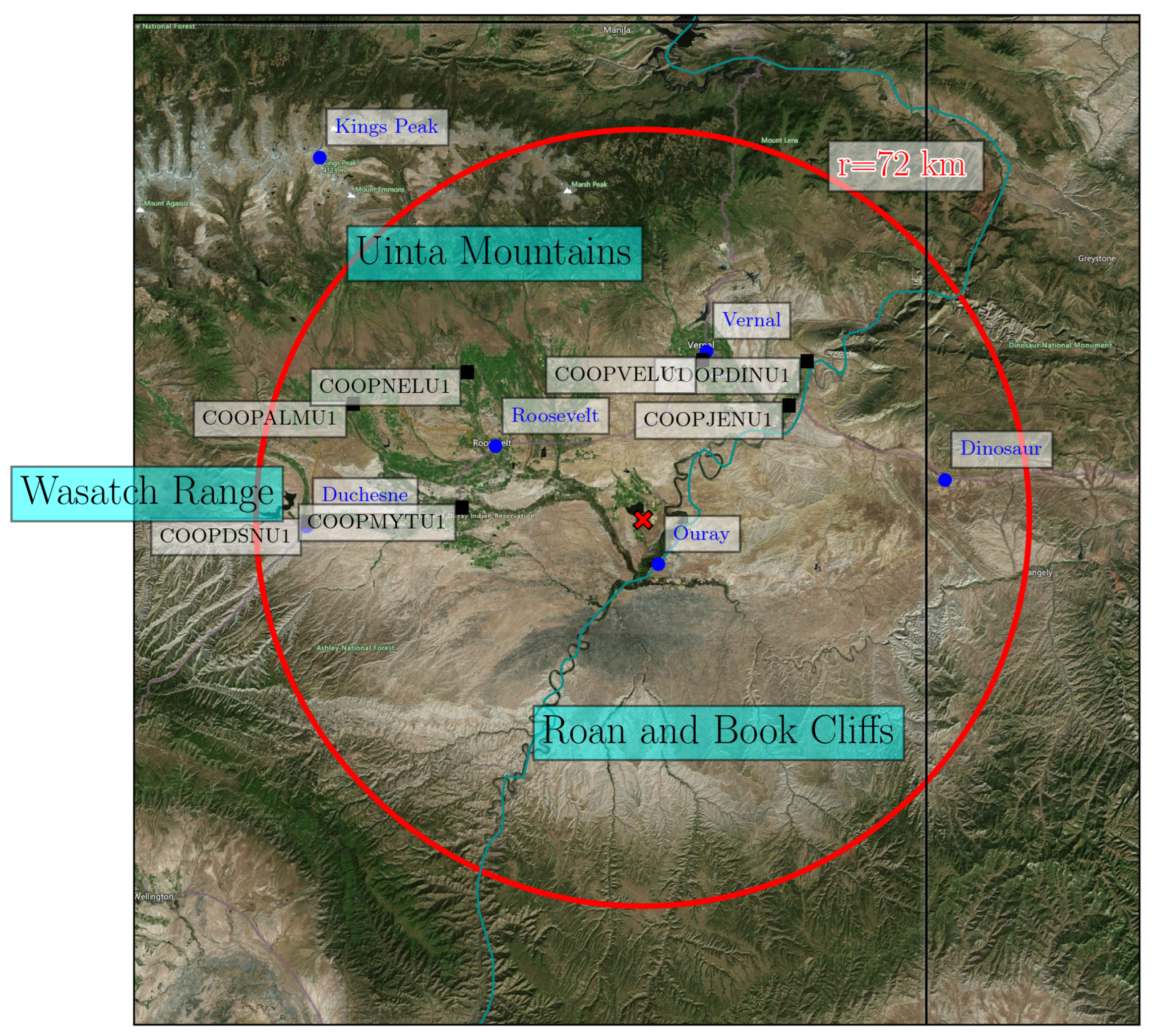
Figure 7.
Membership function for daily maximum of atmospheric ozone concentration.
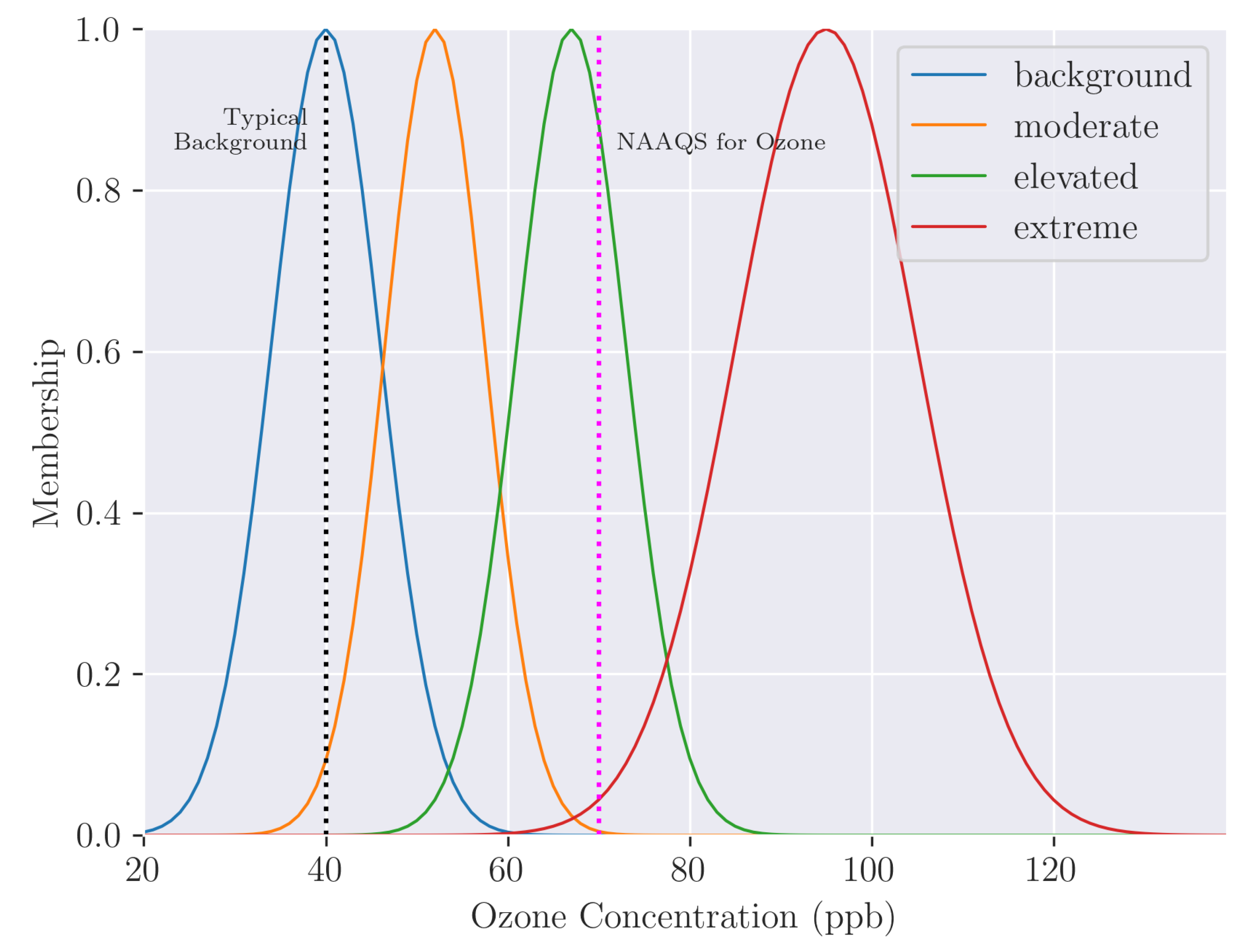
Figure 12.
Full forecast of centroid (best-guess), observed (orange), and four possibility levels overlaid so the higher levels are higher in the stack of bars.
Figure 12.
Full forecast of centroid (best-guess), observed (orange), and four possibility levels overlaid so the higher levels are higher in the stack of bars.
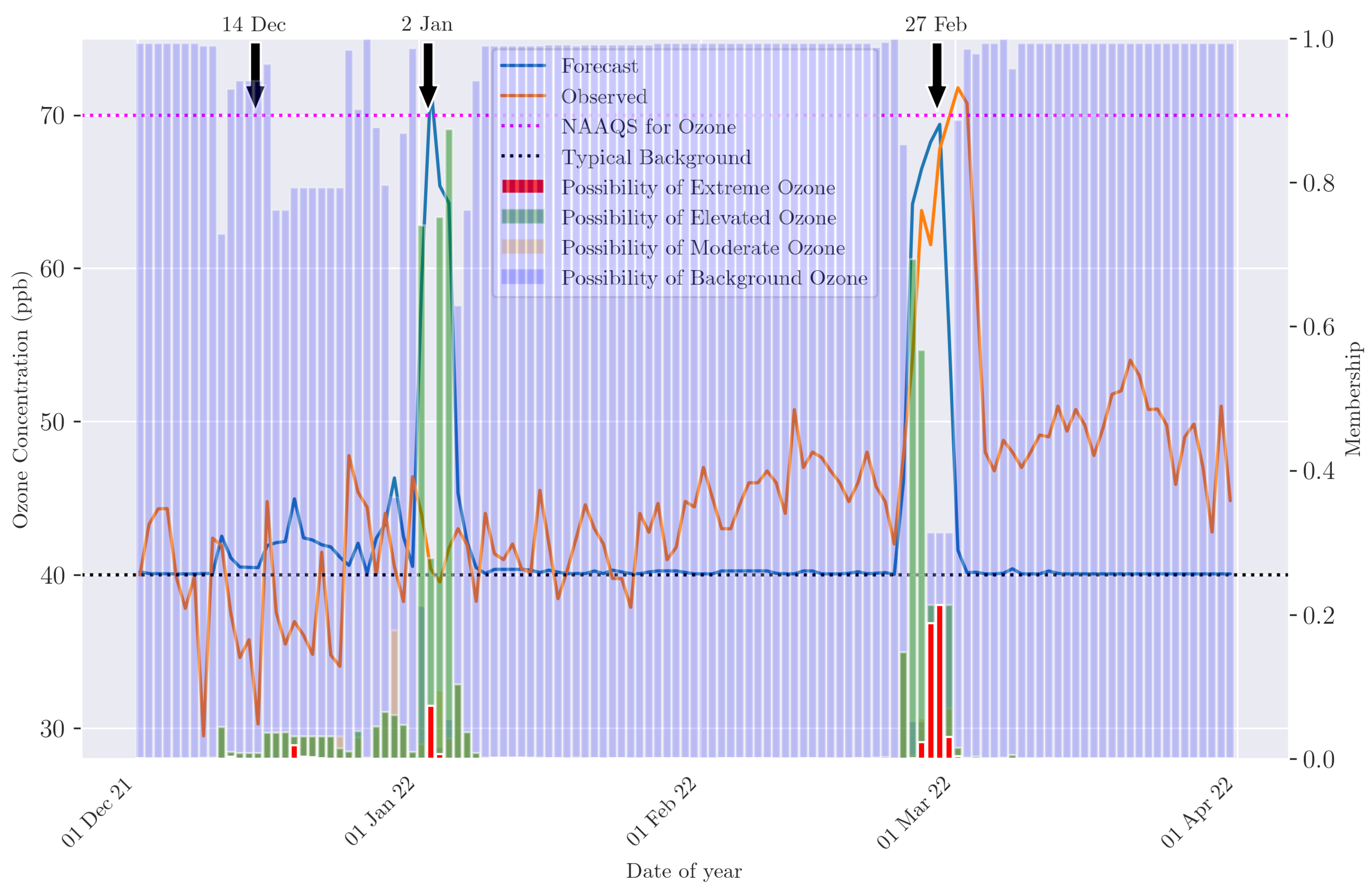
Figure 13.
Forecast of ozone categories valid 14 December 2021, showing background predicted well. F and O denote the rough category that the forecast and observed values fell into, respectively. The annotated rank displays that possibility value’s percentile in this winter’s set.
Figure 13.
Forecast of ozone categories valid 14 December 2021, showing background predicted well. F and O denote the rough category that the forecast and observed values fell into, respectively. The annotated rank displays that possibility value’s percentile in this winter’s set.
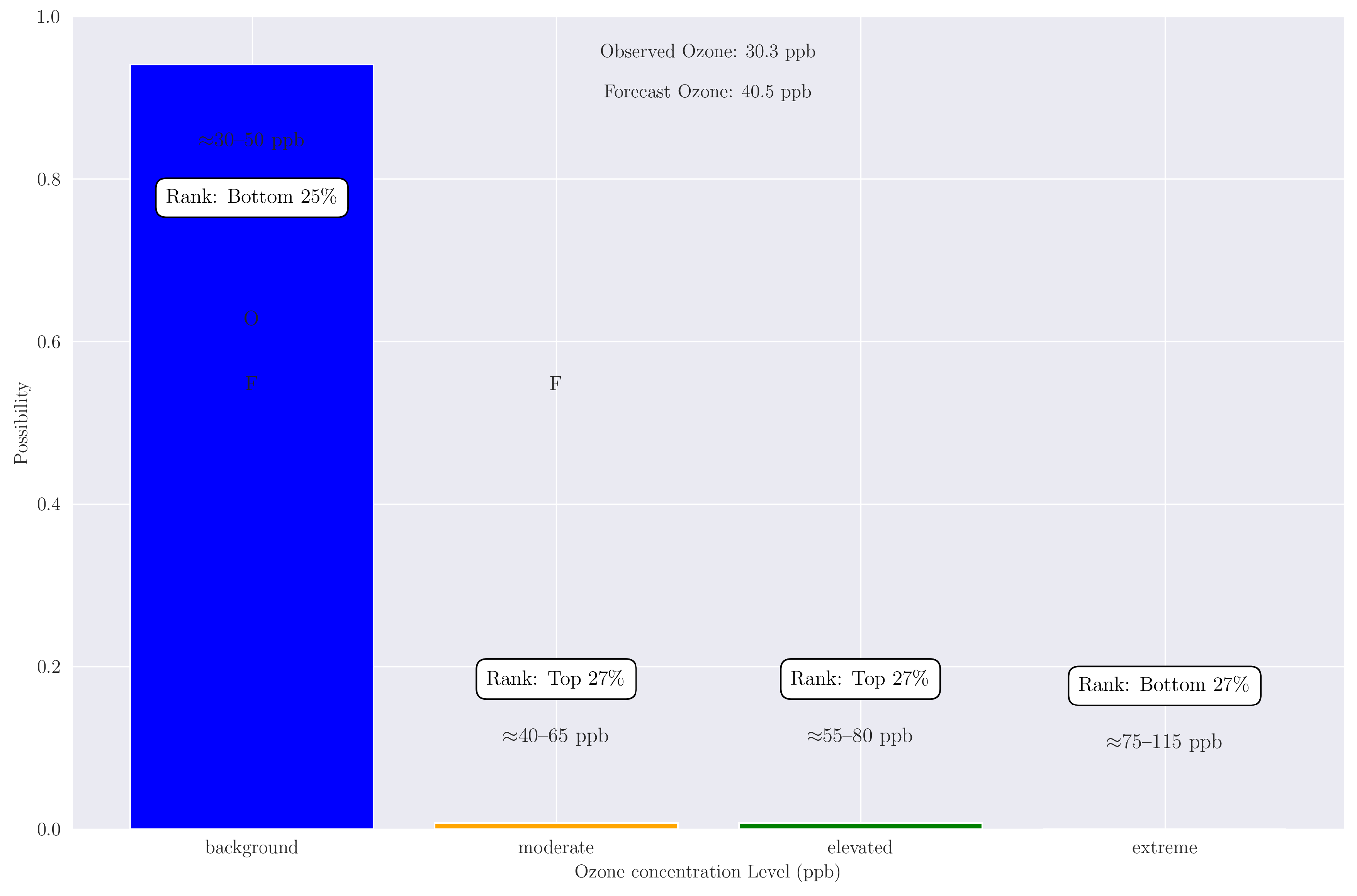
Figure 14.
Forecast of ozone categories valid 2 January 2022, subjectively a poorly forecast case.
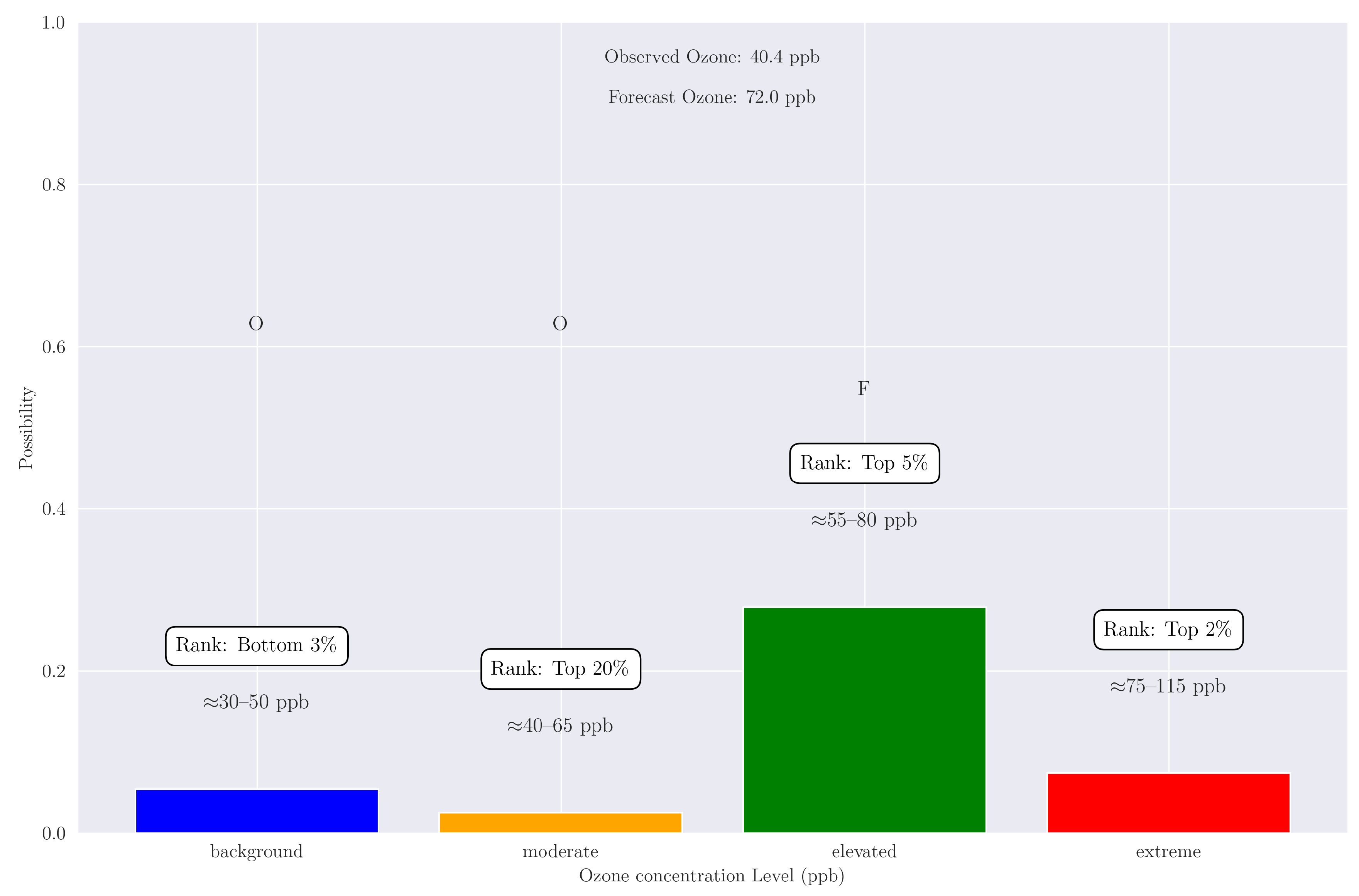
Figure 15.
Forecast of ozone categories valid 27 February 2022. This was a subjectively good forecast, including in the deterministic time series (Figure 12)
Figure 15.
Forecast of ozone categories valid 27 February 2022. This was a subjectively good forecast, including in the deterministic time series (Figure 12)
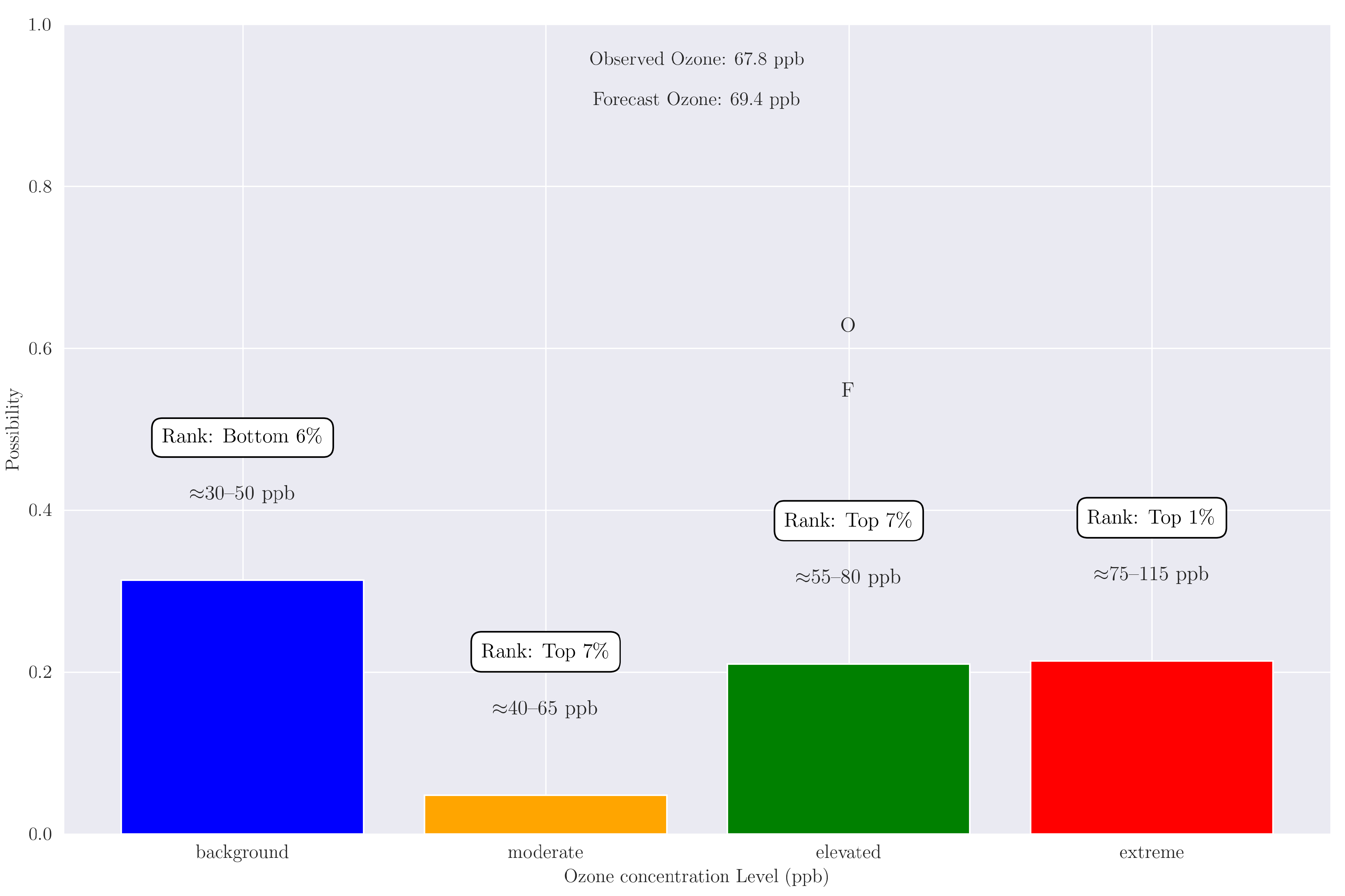
Figure 16.
Box-and-whisker distribution plot for possibility for each category of ozone-concentration daily maximum for the winter 2021/2022. Circles are individual events. Boxes represent the interquartile range.
Figure 16.
Box-and-whisker distribution plot for possibility for each category of ozone-concentration daily maximum for the winter 2021/2022. Circles are individual events. Boxes represent the interquartile range.
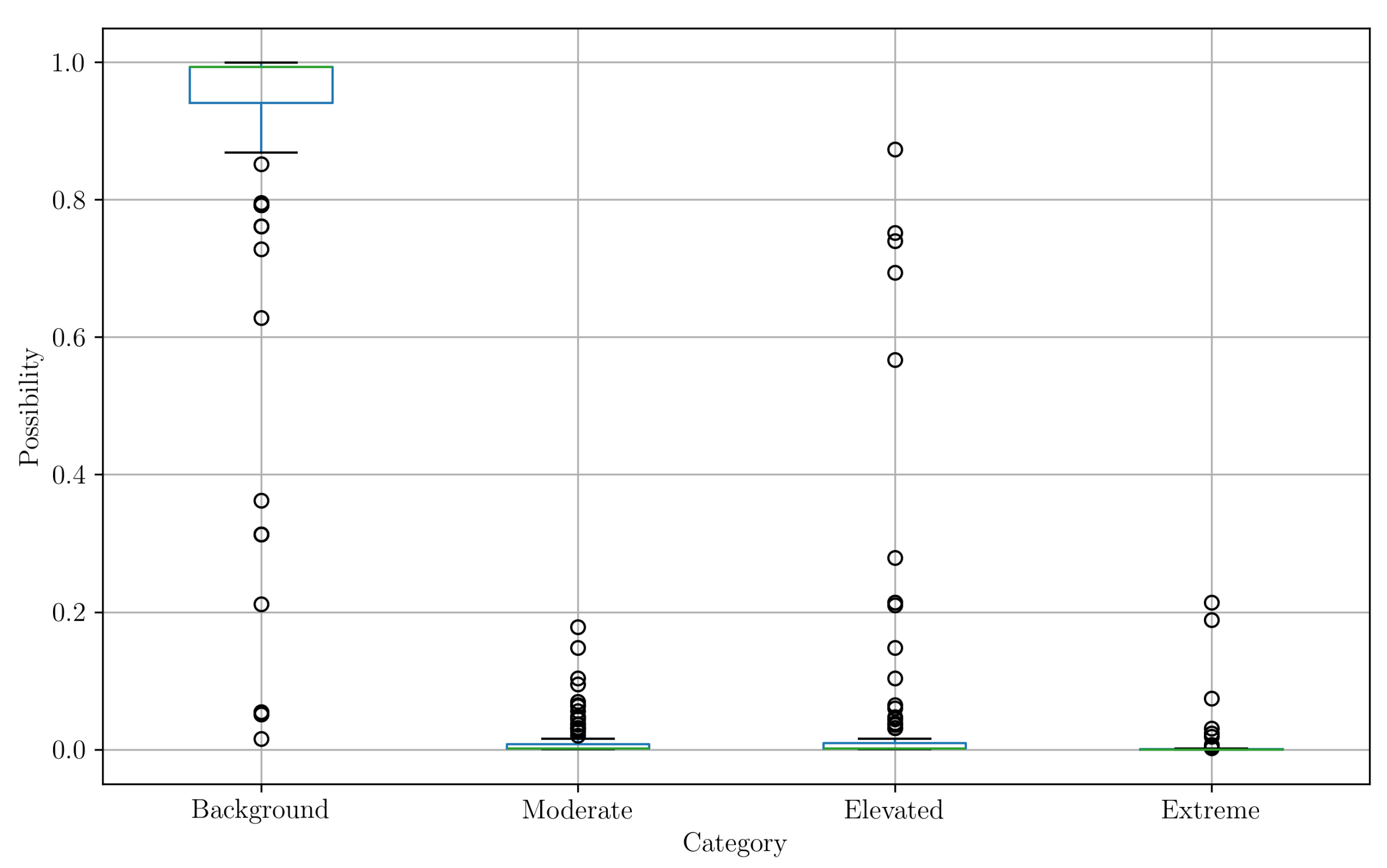
Table 1.
Parameters for membership functions shown graphically in Figure 3, Figure 4, Figure 5, Figure 6 and Figure 7.
| Variable | Units | Category | Function | b | c | ||
| wind | calm | sigmoid | - | - | 2.5 | -3.0 | |
| breezy | sigmoid | - | - | 2.5 | 3.0 | ||
| snow | mm | negligible | sigmoid | - | - | 70 | -0.07 |
| sufficient | sigmoid | - | - | 100 | 0.07 | ||
| mslp | Pa | low | sigmoid | - | - | 101300 | -0.005 |
| average | Gaussian | 102900 | 800 | - | - | ||
| high | sigmoid | - | - | 104500 | 0.005 | ||
| solar | midwinter | sigmoid | - | - | 300 | -0.03 | |
| winter | Gaussian | 450 | 100 | - | - | ||
| spring | Gaussian | 650 | 100 | - | - | ||
| summer | sigmoid | - | - | 750 | 0.03 | ||
| ozone | ppb | background | Gaussian | 40 | 6.0 | - | - |
| moderate | Gaussian | 52 | 5.5 | - | - | ||
| elevated | Gaussian | 67 | 6.0 | - | - | ||
| moderate | Gaussian | 95 | 10.0 | - | - |
Disclaimer/Publisher’s Note: The statements, opinions and data contained in all publications are solely those of the individual author(s) and contributor(s) and not of MDPI and/or the editor(s). MDPI and/or the editor(s) disclaim responsibility for any injury to people or property resulting from any ideas, methods, instructions or products referred to in the content. |
© 2024 by the authors. Licensee MDPI, Basel, Switzerland. This article is an open access article distributed under the terms and conditions of the Creative Commons Attribution (CC BY) license (http://creativecommons.org/licenses/by/4.0/).
Copyright: This open access article is published under a Creative Commons CC BY 4.0 license, which permit the free download, distribution, and reuse, provided that the author and preprint are cited in any reuse.


