Preprint
Article

Carbon Emission Prediction of Transportation Industry in Jiangsu Province Based on WOA-SVM Model

Altmetrics

Downloads

81

Views

17

Comments

0

This version is not peer-reviewed

Submitted:

06 August 2024

Posted:

07 August 2024

You are already at the latest version

Alerts
Abstract
In order to help the transportation industry achieve the goal of carbon peak and carbon neutrality, this study is based on the selection of eight variables, such as population size, per ca pita GDP, personal vehicle ownership, passenger and freight turnover, and green space coverage, as the factors influencing the carbon emissions of the transportation industry in Jiangsu Province, and the prediction and analysis of the transportation carbon emission trends from 2000 to 2021, and the prediction and analysis of the carbon emissions of the transportation industry and the time of the peak of the carbon emissions in Jiangsu Province. The trend of transportation carbon emissions from 2000 to 2021 was predicted and analyzed, and the carbon emissions and peak time of carbon emissions in the transportation industry in Jiangsu Province were predicted and analyzed. Comparing the predicted results with other models to verify the accuracy of the results, it was found that the WOA-SVM model had the smallest error among several models. On this basis, targeted measures are proposed to accelerate the process of carbon peak and ensure the smooth achievement of carbon neutrality goals in Jiangsu Province. The results indicate that under the current policy measures, the peak carbon emissions in Jiangsu Province will occur in 2038, with a peak of 48.72 million tons. Jiangsu Province should actively adopt energy-saving and emission-reduction measures, build a green and low-carbon transportation development model, and achieve the carbon peak target ahead of schedule.
Keywords: 
Subject: Business, Economics and Management  -   Human Resources and Organizations

1. Introduction

Global warming has become a major challenge facing humanity today, and it has become a global consensus that the increase in the concentration of greenhouse gases, represented by carbon dioxide, is the main cause of climate warming, and all countries have taken energy-saving and emission reduction measures to cope with this common challenge. Since the reform and opening up, China has made world-renowned achievements in economic construction and rapidly accelerated the process of urbanization. However, with the increasing consumption of resources, negative impacts such as environmental pollution and large carbon emissions have ensued. Since China’s carbon emissions surpassed those of the United States in 2006, it has become the country with the largest carbon emissions for 14 consecutive years. Its carbon emissions are far ahead of the United States, which is the second largest in the world [1] (pp. 63250-71). As the leader of developing countries, reducing China’s carbon emissions is important for promoting sustainable growth of the domestic economy and an important initiative to cope with global climate change. For this reason, the Chinese government has proposed the "dual carbon" goal to achieve a carbon peak before 2030 and carbon neutrality before 2060.
In recent years, scholars have mainly conducted comprehensive research on the factors influencing carbon emissions, research methods, and prediction models related to the carbon peak in the transportation industry. To identify the influencing factors of carbon emissions in transportation, Fan [2] (pp. 135-45) constructed a multivariate generalized Fisher index (GFI) decomposition model and classified the influence of related factors into positive drivers, negative drivers, and general constituents according to the contribution rate of carbon emissions; Xu [3] (p. 664046) explored the driving factors of carbon emissions in the transportation industry in terms of spatial correlation of CO. The study found that under the influence of the drivers, the carbon emissions tend to increase from north to south; Rasool [4] (pp. 22907-21) used regression allocation lag model and Granger causality vector error correction model to analyze the causal relationship between factors and carbon emissions. The results showed that population plays a dominant role in carbon emissions in the transportation industry, and the transportation system and energy structure should be adjusted to reduce carbon emissions. As for the research on carbon peak prediction, from the perspective of research methods, most scholars mainly based on the analysis of different scenarios and the establishment of prediction models to predict the time of carbon peak and portray the path of carbon peak and the methods commonly used by academics for carbon emission prediction mainly include gray prediction model, STIRPAT model, and system dynamics model, and time series model, etc. Chai et al. [5] (pp. 1-16), Yin [6] (p. 136889), Wang et al [7] (p. 136221) used the STIRPAT model, gray prediction model, and system dynamics model to forecast carbon emissions, respectively, and among the time series models, the most commonly used model is ARIMA model. Modise used the ARIMA model to determine the baseline demand for future transportation manufacturing and carbon emissions generated by electricity, considering the errors that may create changes in demand [8] (p. 8466). And innovatively applied the prediction of energy and carbon emission efficiency to the data monitoring system of transportation manufacturing to control the carbon emission of the transportation industry. Ning [9] (p. 1441942) predicted the carbon emissions of four representative cities in China, namely Beijing, Henan, Guangdong, and Zhejiang, over the next three years by constructing an ARIMA model, using white noise testing and error analysis.
The related factors are analyzed, and relevant suggestions are made according to the socioeconomic conditions. With the continuous deepening of research, predictive analyses on support vector machine models incorporating Whale Optimisation Algorithm (WOA-SVM) representations have also been increasing. Zhou [10] (pp. 3654-64) compared the WOA-SVM model with Support Vector Machine (SVM), Decision Tree (DT), K-Nearest Neighbours (KNN) HE Support Vector Machine combined with Loop Optimization Algorithm (LOA-SVM) model, and proved that the WOA-SVM has a higher prediction accuracy, and the analysis speed is fast, good repeatability With the rapid development of artificial intelligence, machine learning methods are widely used in the transportation sector in carbon emission prediction. Machine learning uses mathematical methods to extract features from huge amounts of data to solve highly complex classification and regression problems. Ağbulut [11] (pp. 141-57) uses three machine learning algorithms to analyze and predict Turkey’s transport carbon emissions. This structure shows that by 2050, the transport sector’s carbon emissions will increase by 3.4 times over the current level. There is an urgent need to adjust the energy structure to reduce the carbon emissions from transportation. Developing supercharging and other regression models based on machine learning to improve the carbon emissions of light-duty vehicle designs and creating integrated learning models for predicting carbon emissions using vehicle specifications provide essential insights into air pollution from transportation.
In summary, research on carbon emissions has mainly focused on analyzing its influencing factors and predicting emissions based on traditional algorithms in the past. However, with the vigorous development of machine learning technology, numerous new algorithms have emerged, among which support vector machine (SVM) stands out among many algorithms and demonstrates significant advantages. SVM, as an algorithm suitable for learning small sample data, is highly compatible with the characteristics of small sample datasets commonly faced in the field of carbon emissions. At the same time, its strong robustness is particularly critical. It can effectively deal with individual year data anomalies caused by external factors such as policy adjustments and economic fluctuations, ensuring the stability and accuracy of predictions.
The innovative contributions of this article are mainly reflected in the following aspects: firstly, creatively utilizing the small sample learning ability and robustness characteristics of SVM to predict carbon emissions, effectively overcoming the challenges brought by data scarcity and uncertainty. Secondly, in the parameter optimization process of SVM, the traditional grid search method was abandoned, and the Whale Optimization Algorithm (WOA) was adopted instead. This algorithm combines the breadth of global search with the refinement of local search, significantly reducing the risk of falling into local optimal solutions and improving the efficiency of optimal parameter configuration in the model. Finally, in response to the complex growth trends that are difficult to capture in historical carbon emission data directly, this article innovatively combines the grey prediction model. By complementing the advantages of both models, the ambiguity of the prediction results is effectively reduced, and the accuracy of long-term predictions is improved.

2. Models and Methods

2.1. Whale Optimization Algorithm Model

2.1.1. Algorithm Overview

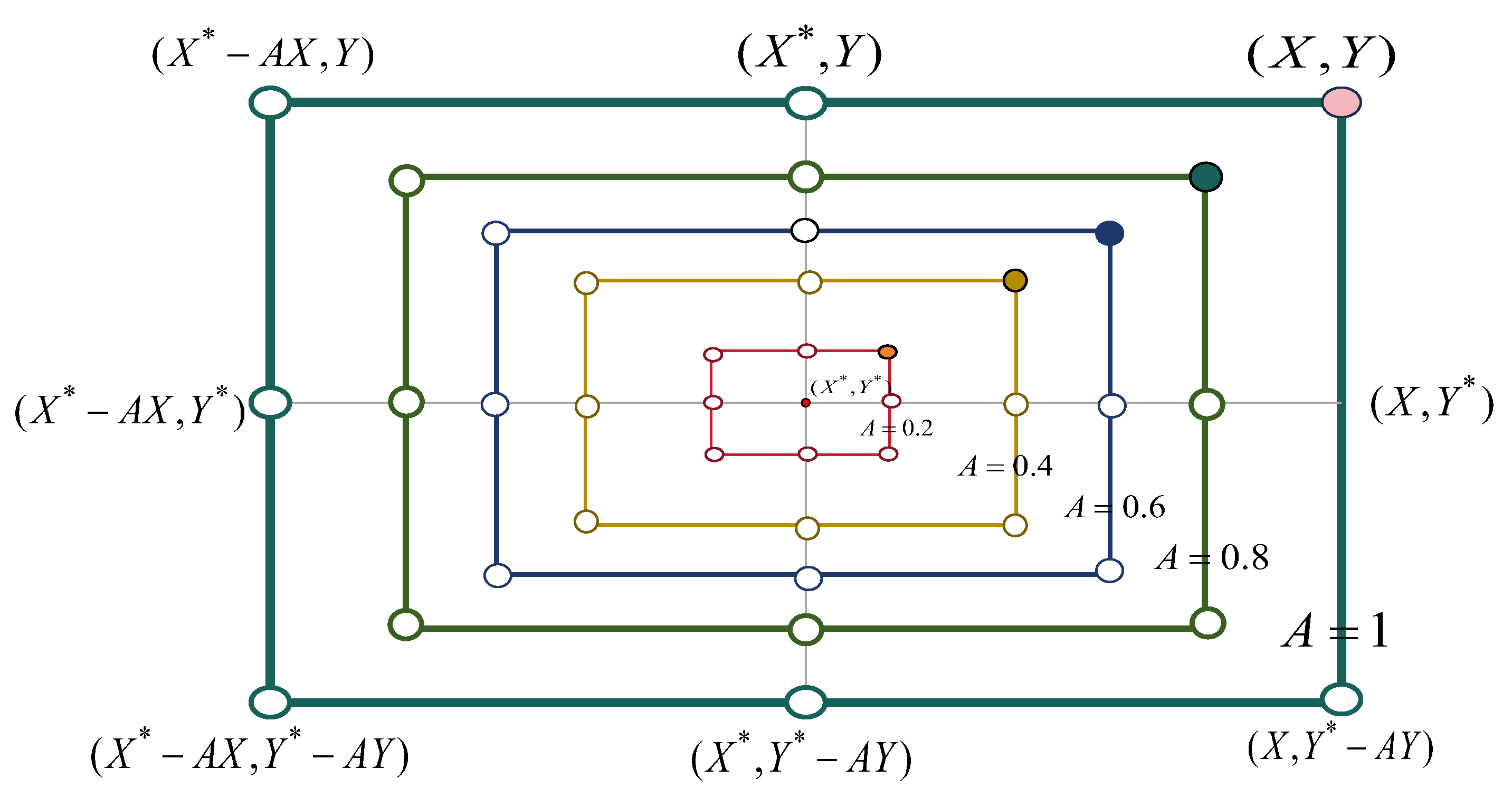
Whale optimization algorithm (WOA) [12] (pp. 51-67) is an emerging algorithm proposed based on the behavior of whales hunting prey. In the whale algorithm, the position of each whale represents a feasible solution. In the process of whale hunting, each whale has two behaviors. One is to surround the prey, and all whales move towards other whales. Another type is the steam drum net, where whales swim in a circular motion and release bubbles to drive away prey. In each generation of swimming, whales randomly choose these two behaviors to hunt. In the behavior of surrounding prey, whales will randomly choose whether to swim toward the optimal position or randomly select a whale as their target and approach it.

2.1.2. Encirclement Predation Method

When hunting, whales choose to swim to the best or a random whale position. This will be determined by the modulus of the D-dimensional vector A, When |A <1|, whales choose to swim towards the optimal individual. So when the modulus of A is less than 1, the whale swims towards the optimal individual.When |A >1|, whales choose to swim towards random individuals.It can be seen that during the process of surrounding prey, the whale algorithm’s search mode is to search around the optimal individual or near the random individual [13] (pp. 96273-83).
a) Swimming towards the optimal position for the whale
D = | C X ( t ) * X ( t ) |
X ( t + 1 ) = X ( t ) * A D
where D represents the distance between the prey and the whale, t represents the current iteration number, X(t) represents the global optimal position (i.e. the position of the prey) at the iteration t, and X(t) and X(t+1) represent the position of the whale at the iteration t and t+1, respectively. A and C are coefficients used in the algorithm to adjust the movement and search behavior of the whale. The values of A and C are as follows:
A = 2 a r a a   ;   C = 2 r c a = 2 2 t / T m a x
In the formula,  r a  and  r c  are random vectors in the interval [0,1] used to introduce randomness into the iteration; a is the convergence factor, the value of which decreases linearly from 2 to 0 as the number of iterations increases from 0 to Tmax (maximum number of iterations) according to formula (3), thereby affecting the value of A and regulating the whale’s search behavior from global exploration to local search.
Figure 1. Diagram of Encirclement Attack.
Preprints 114443 g001
b) Swimming towards a random location for whales
During the search, the whale also sets the search range for the prey to a random range in order to determine the location. When A>1, the whale searches for prey randomly in the global range, improving the global optimization ability [14] (pp. 69688-99). The process is as follows:
D = | C X r a n d X ( t ) |
X ( t + 1 ) = X r a n d A D
In the formula,  X r a n d  is the whale position vector for random search, and  D  is the distance between the current search individual and the random individual.

2.1.3. Bubble-Net Attacking Method

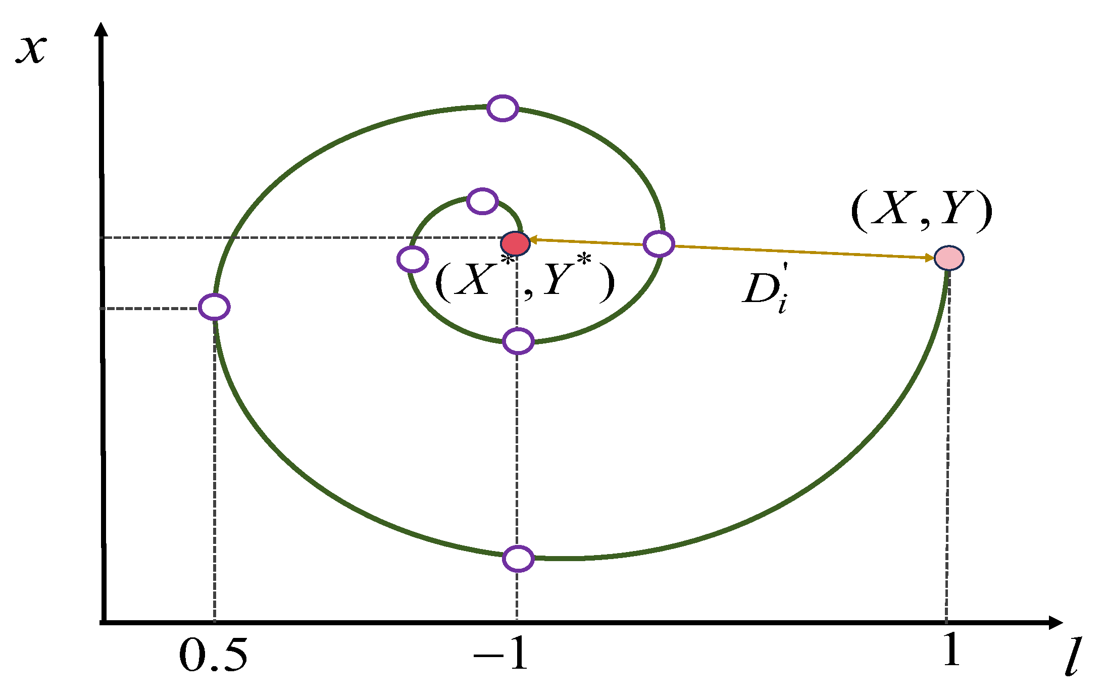
Another way that whale pods hunt is by approaching prey along a spiral path, releasing bubbles to form a bubble net. The mathematical model describes how whales calculate the spiral trajectory to update their position, approach prey, and reflect the bubble effect through position adjustment or search strategies [15] (pp. 6439-52). The mathematical model is as follows:
X ( t + 1 ) = X ( t ) * + D e b l cos ( 2 π l ) D = | X ( t ) * X ( t ) |
where D defines the distance between the i-th whale and the prey, b defines the shape of the spiral, and l is a random number in the range [−1,1].
The probability of the two predatory behaviors (encircling and spiral approach) occurring in the population is 50% each, ensuring diversity and efficiency in the search process.
Figure 2. Diagram of Bubble Network Attack.
Preprints 114443 g002

2.2. Principle of Support Vector Machine

Support Vector Machine (SVM) [16] (pp. 207-35) has been a revolutionary technology in supervised learning since its introduction in 1995 and is widely used in classification and regression. The basic principle is that in the context of regression problems, we consider a given training sample set, where the variables (or feature vectors) represent the independent variables, the dependent variables (or target values) represent the dependent variables, and N represents the sample size. In an SVM regression model, the goal is to find a hyperplane (or a generalization of a hyperplane in high-dimensional space) [17] that best fits the training data while maintaining prediction accuracy for unseen data. Unlike the optimal separating hyperplane in a classification problem, the goal of an SVM regression model is to minimize the distance of all training sample points to the hyperplane while allowing some deviation (i.e., a non-sensitive loss function) to handle noise and outliers in the data.

3. Transportation Carbon Emission Prediction Modeling

Specifically, SVM regression seeks a hyperplane so that most data points fall between two hyperplanes parallel to the hyperplane (so-called -tubes) while minimizing the number of data points that lie outside the tubes or their distance from the tube boundaries. In this way, the SVM regression model can balance the complexity of the model and the degree of fit to the data, thereby exhibiting good generalization when dealing with regression tasks. The regression model is as follows:
f ( x ) = ω × x + b
where  f ( x )  is the output variable of the model;  ω  is the feature space weight vector;  x  is the input variable; and  b  is the bias vector. The structural risk function expression used in the SVM regression model is as follows:
R ( f ) = 1 2 ω 2 + C i = 1 m L ε [ f ( x i ) y i ]
where  C  is the penalty factor,  m  is the sample size,  L ε  is the insensitive loss function of  ε ε  is the loss factor of the loss function, and the SVM regression function is as follows.
f ( x ) = i = 1 m a i K ( x i , x ) + b
where  a i  is the Lagrange multiplier of the ith sample and  K ( x i , x )  is the inner product, i.e., the kernel function. For the inner product problem, the RBF kernel function, which is widely used, is adopted, and the expression is as follows:
K ( x i , x ) = e x p ( g x i , x ) , g > 0

3.1. Selection of Indicators

The STIRPAT model is expanded from the IPAT mode [18] (p. 111328) to study the impact of factors on environmental loads by quantitative analysis. Multiple independent variables related to scale, structure, and technology can be introduced into the model. In the process of using the STIRPAT model to study the carbon emissions, other factors that may impact the carbon emissions can be introduced based on the actual situation of the study area. The expression is shown in equation [19] (pp. 1667-85):
I = a × P b × B c × T d × e
where is the constant term; is the exponential term for P, B, and T, respectively; e is the error term; and is the environment, population, economy, and technology, respectively.
Summarized through the literature, carbon emissions from transportation are affected by population, economy, technology, and transportation itself [20] (p. 8848149). Zhu [21] (p. 8610) studied the influence of population size, economic growth, and energy intensity on transportation carbon emissions; Xu [22] (pp. 311-22) selected economic growth, urbanization rate, the number of private cars, cargo turnover, and energy efficiency as the key factors affecting the carbon emissions of the transportation sector to be analyzed; Xu X [3] (p. 664046) believed that the transportation intensity, the level of urbanization, the level of technology, the per ca-pita GDP, and the industrial structure have a direct role in the carbon emissions. Emission. Therefore, based on the STIRPAT model and the results of existing studies on the factors affecting carbon emissions, this study, combined with the availability of data, selected eight variables from the four dimensions of population, economy, technology, and transportation: total population, per ca-pita GDP, motor vehicle ownership, passenger turnover, cargo turnover, urbanization rate, urban green space coverage, and carbon emission intensity as The main factors affecting carbon emissions in Jiangsu Province transportation industry. Among them, carbon emission intensity refers to the transportation carbon emission brought by the growth of unit GDP.

3.2. Transportation Carbon Emissions Measurement

This paper adopts the “top-down” carbon emission calculation method in the “IPCC 2006 Guidelines for National Greenhouse Gas Inventories” [23] (p. 5395) to calculate carbon emissions from transportation based on transportation fuel consumption combined with input-output analysis and carbon emission factor accounting methods, and the calculation formulas are as follows [24] (pp. 65-71):
C = i C i = i E i × F i = i E i × A L V i × C V i × C O F i × 44 12
Among them is the type of energy, which is divided into raw coal, gasoline, diesel, electricity, natural gas, fuel oil, liquefied petroleum gas, etc., the consumption of the type of energy, the carbon emission coefficient of the kind of energy, is the average status of heat generation, is the carbon content per unit of calorific value, is the rate of carbon oxidation, 44/12 is the molecular weight of carbon and, and the average low status of heat generation of each type of energy, carbon content per unit of calorific value, and the rate of carbon oxidation are referred to the “Statistical Survey System of Energy Resource Consumption by Public Organizations.” Energy Resources Consumption Statistics Survey System for Public Organizations” [25], and the data are from China Energy Statistics Yearbook [26] (p. 131417). The energy carbon emission coefficients used in this paper are shown in Table 1.

3.3. Transportation Carbon Emissions Projections

First, the time series data of the selected eight indicator variables and emissions are normalized to remove dimensional differences. Second, the whale optimization algorithm is set to a maximum number of iterations of 50, a population size of 50, and a logarithmic spiral shape constant b of 1. The parameter settings c and g are set to [0.001,5000] and [0.001,1000]. For the support vector machine, the fitness function is the prediction’s mean square error (MSE).
In order to compare the testing ability and accuracy of multiple evaluation models, this paper uses RMSE (root mean square error) and MAPE (mean absolute percentage error) to analyze the prediction model. The smaller the RMSE and MAPE, the more accurate the model’s prediction results. The calculation formulas are as follows:
R M S E = 1 n i ( y i y ^ i ) 2
M A P E = 100 % n i = 1 n | y i y ^ i y i |

4. Empirical Analysis of Transportation Carbon Emission Forecasts in Jiangsu Province

4.1. Characteristics of Spatial and Temporal Distribution of Carbon Emissions from Transportation Industry in Jiangsu Province

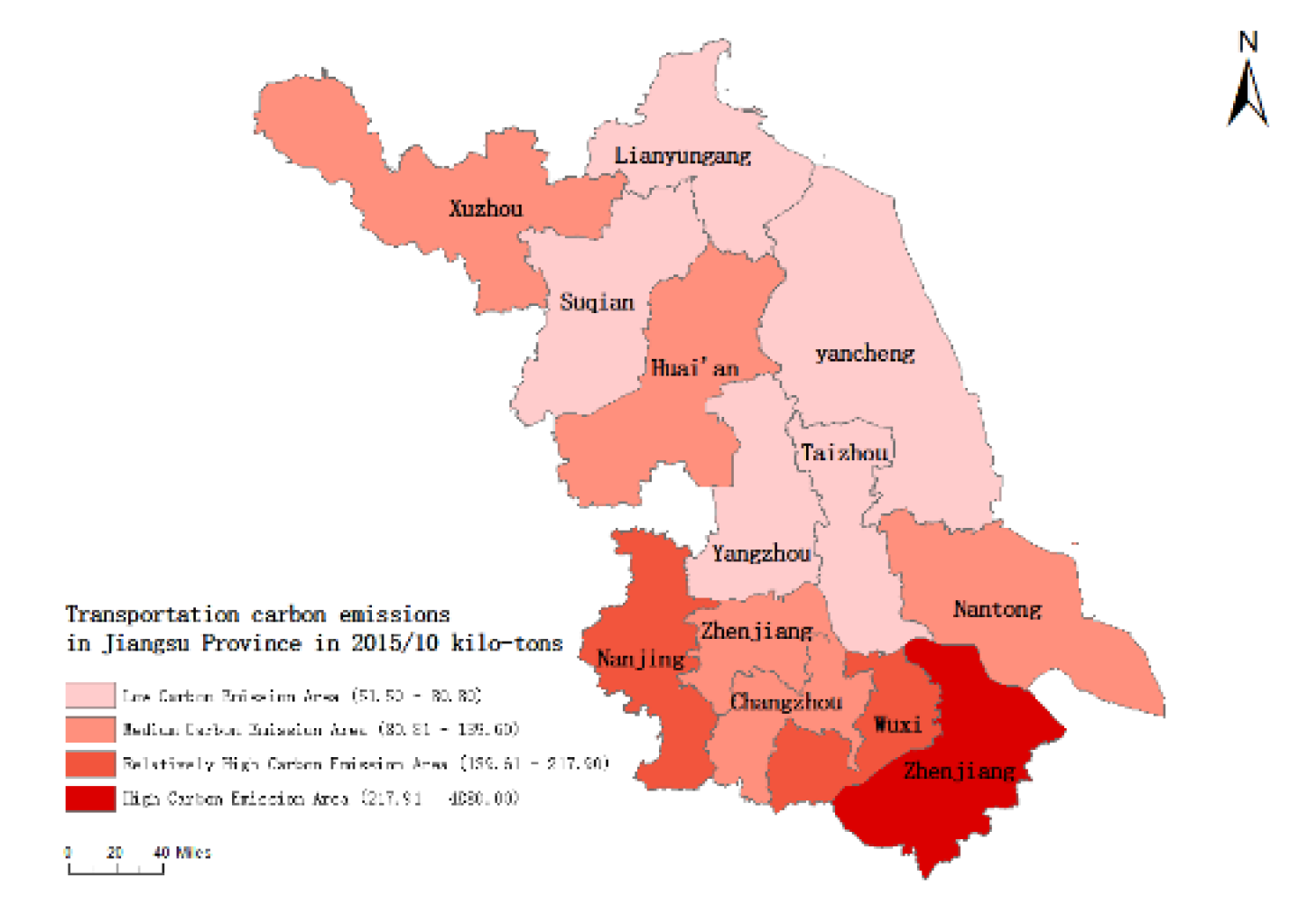
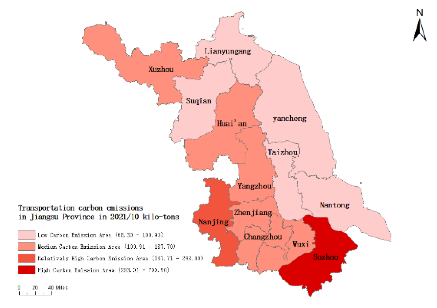
In order to explore the spatial distribution pattern and temporal changes of carbon emissions in the transportation industry of various cities in Jiangsu Province, this paper quantifies the carbon emissions of the transportation industry of Jiangsu Province in 2015 and 2021, respectively, using the natural breakpoint method of ArcGIS software, and divides the 13 cities in Jiangsu Province into high carbon emission zones, higher carbon emission zones, medium carbon emission zones, and low carbon emission zones. As shown in Figure 3 and Figure 4.
From the distribution of total carbon emissions from the transportation industry in Jiangsu Province in 2015 and 2021, the carbon emissions of all cities in Jiangsu Province generally show the distribution of "high in the south and low in the north," and the carbon emissions of Suzhou are much higher than those of other cities. It is the only high carbon emission zone in Jiangsu Province. With the support of the National 12th Five-Year Plan, each region has formulated relevant energy-saving, carbon-reduction, and emission-reduction programs based on the actual situation, and the transportation industry has started to take more stringent energy-saving and emission-reduction measures. Among them, Nantong and Wuxi have significantly reduced emissions, with Wuxi moving from a high carbon emission zone to a medium carbon emission zone. Nantong moving from a medium carbon emission zone to a low carbon emission zone, proving the efficiency of energy-saving and emission-reduction measures and the achievability of the "dual-carbon goal" through practical actions.

4.2. Analysis of Influencing Factors of Transport Carbon Emission in Jiangsu Province

1. Example data selection and calculation of transportation carbon emissions
According to the existing research, this paper selects eight influencing factors, namely, total population, per capita GDP, motor vehicle ownership, passenger turnover rate, cargo turnover rate, urbanization rate, urban green space coverage rate, and carbon emission intensity, to construct a measurement system of influencing factors of transportation carbon emission in Jiangsu Province, as shown in Table 2. According to the national release of the "China Energy Statistics Yearbook" under the regional energy balance table of Jiangsu energy balance table [27] (p. 813), the relevant energy transportation consumption is obtained. According to the above formula to calculate the carbon emission energy consumption data of the transportation industry in Jiangsu Province, the specific value is shown in Table 3.
2. Data covariance diagnosis and dimensionality reduction
The research data in this paper were analyzed by the multicollinearity test, using the VIF test, where the VIF value indicates the variance inflation factor, the tolerance value is the reciprocal of the VIF value, and the severity of multicollinearity is measured by these two indicators. It is generally considered that if the VIF value is greater than ten or the tolerance value is less than 0.1, there is a multicollinearity problem, and the specific analysis results are shown in Table 4.
As shown in Table 4, the VIF values of the eight variables under study are all greater than 10, indicating a serious multicollinearity problem among these variables. In order to overcome the adverse effects of variable multicollinearity in the modeling process, this paper uses principal component analysis to decompose the original eight variables and extract the principal components to establish a regression model as an alternative to the original model structure.
The number of principal components was extracted based on the cumulative variance value to determine, as shown in Table 5, four principal components were finally resolved, and the value is 99.628, which explains the original model well, so the four principal components (U1, U2, U3, U4) are used to represent the eight indicator factors, The regression equation is obtained as shown in Table 5, the coefficients of these four principal components are different and uncorrelated with each other, and according to the regression equation, the eight covariate variables will be transformed into four independent variables to realize the downgrading of the indicator system. The following calculations are all carried out based on these four independent variables. The following calculations are based on these four independent variables.
U 1 = 0.382 * C 1 + 0.364 * C 2 + ( - 0.277 ) * C 3 + 0.370 * C 4 + 0.274 * C 5 - 0.364 * C 6 + 0.387 * C 8 + 0.388 * C 8
U 2 = ( 0.244 ) * C 1 + ( 0.38 ) * C 2 + ( 0.563 ) * C 3 + 0.293 * C 4 + ( - 0.512 ) * C 5 + ( - 0.295 ) * C 6 + 0.205 * C 7 + ( - 0.039 ) * C 8
U 3 = 0.072 * C 1 + ( - 0.04 ) * C 2 + 0.623 * C 3 + 0.065 * C 4 + 0.738 * C 5 + 0.031 * C 6 + ( 0.032 ) * C 7 + ( - 0.233 ) * C 8
U 4 = ( - 0.205 ) * C 1 + ( - 0.071 ) * C 2 + 0.386 * C 3 + ( - 0.085 ) * C 4 + ( - 0.293 ) * C 5 + ( 0.83 ) * C 6 + ( - 0.076 ) * C 7 + ( 0.129 ) * C 8

5. Simulated Prediction of Transport Carbon Emissions Based on WOA-SVM Models

5.1. WOA-SVM Model Simulation Prediction

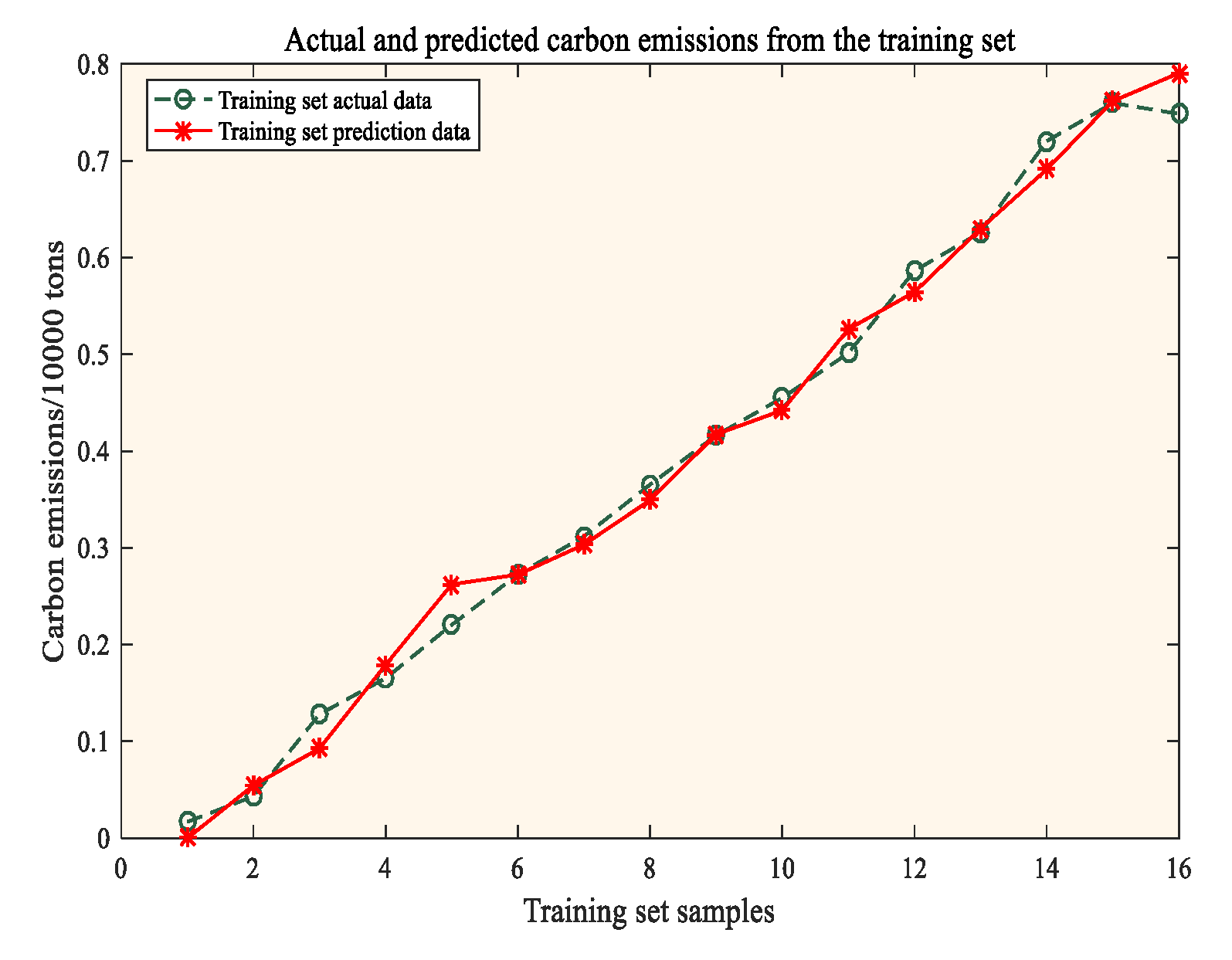
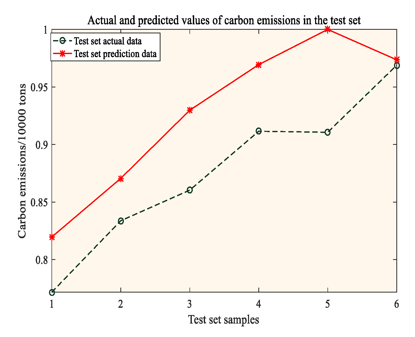
Above, the original primary data of energy consumption in the transportation industry from 2000 to 2021 are normalized, correlation analyzed, and factorized to form a new data matrix from 2000 to 2021. This paper selects the 2000-2014 data as the training samples to train the WOA-SVM model, and the 2014-2021 data are taken as the test samples. MATLAB programming simulation is used to calculate the running curve of the fitting results and the running curve of the relative error of the test set data, as shown in Figure 5 and Figure 6.
From the training set and validation set errors in the above table, it can be concluded that the WOA-SVM model can predict the trend of carbon emissions well, and the model predicts a minor error, from which it can be concluded that the WOA-SVM model prediction model has high discriminatory accuracy and the model is more stable.

5.2. Comparison of Three Simulation Predictions

To verify the effectiveness of different models in predicting CO2 emissions from the transportation industry in Jiangsu Province, four regression prediction models were constructed and compared: LSTM (time series prediction model), unoptimized SVM model, GA-SVM (genetic algorithm optimized SVM model), and WOA-SVM (whale optimized vector machine model) for regression prediction to analyze and compare the four models. The mean absolute percentage error (MAPE) and the root mean square error (RMSE) [28] (pp. 5912967) of the test set were used as evaluation indicators. The results are shown in Table 6.
Table 6 clearly shows that the MAPE and RMSE values of the WOA-SVM prediction model used in this paper are lower than those of the other three prediction models. In summary, the WOA-SVM prediction model has higher prediction accuracy and precision than the other models, and can more accurately predict the carbon emissions of the transportation industry in Jiangsu Province.

5.3. Scenario Simulation

In September 2021, the "14th Five-Year Plan" for Green Transportation Development in Jiangsu Province was officially issued. The Plan specifies that carbon emissions from transportation in Jiangsu Province will reach a carbon peak in 2035. In this paper, we select eight factors, namely, total population, per ca-pita GDP, motor vehicle ownership, passenger turnover rate, cargo turnover rate, urbanization rate, green space coverage in built-up areas, and carbon emission intensity, and make predictions for the next 30 years, i.e., 2022-2051, under the premise of good fitting results and validity test results of the WOA-SVM model, to investigate the situation of transportation carbon emissions in Jiangsu Province during this period, the peak and the year of reaching the peak, and make references to the data of Jiangsu Province Transportation Carbon Emissions Plan. The low, baseline and high carbon scenarios are set for the eight influencing factors concerning many bulletins and policy documents, as shown in Table 5. Relevant references are as follows.
(1) Population: On May 31, 2021, China’s three-child birth policy began to be implemented, and to a certain extent, the population growth of Jiangsu Province played a specific role in the stimulus. According to the seventh population census data of Jiangsu Province, the total resident population of the province is 84.748 million, with a growth rate of 0.75%, and the population increment and incremental growth remain stable; however, concerning the experience of the fertility potential brought about by the "comprehensive two-child" policy, it is presumed that the stimulus brought about by this policy will be released in 3~5 years. The China Population and Development Research Center predicts that China’s population will peak at 1.417 billion in 2027, after which it will enter a sustained negative growth phase [29] (p. 155060).
(2) Per ca-pita GDP. Jiangsu Province’s comprehensive economic strength in the "12th Five-Year Plan" period has been significantly improved; the per ca-pita GDP ranked first in the country, more than 88,000 yuan [30] (p. 126187), the province’s per ca-pita GDP from 66,500 yuan in 2012 to 137,000 yuan in 2021, with an average annual growth rate of 6.8%, in recent years, Jiangsu Province continues to optimize the industrial structure, expand domestic demand, increase the domestic impetus for economic growth, which has a strong driving effect on economic growth. In recent years, Jiangsu Province has been optimizing its industrial structure, expanding domestic demand, increasing the endogenous power of economic growth, and driving economic growth strongly. China’s "14th Five-Year Plan" and the proposed vision for the 23rd Five-Year Plan also clearly set out the goal of doubling economic growth or per capita income by 2035.
(3) Cargo turnover. Under the background of the temperature advancement of the construction of major transportation projects and the stable and healthy operation of the transportation economy, the cargo turnover volume of Jiangsu Province increased steadily between 2000 and 2020, and the cargo turnover volume of Jiangsu Province was 368,779 million ton-kilometers in 2021, an increase of 4.63% year-on-year. According to Liu Jiancui’s measurement of China’s cargo turnover [31] (p. 118892), it can be seen that Jiangsu Province’s cargo turnover maintains a growth rate of about 5% between 2022~2030, and the growth rate is about 3% between 2030~2050.
(4) Passenger turnover. 2020 domestic passenger turnover by the impact of the epidemic fell sharply; the epidemic economic recovery, in recent years, with the development of tourism, passenger turnover in Jiangsu Province increased rapidly; 2021, passenger turnover of 114.21 billion person-kilometers, an increase of 8.04%, 2023 passenger turnover as high as 152.7 billion person-kilometers, an increase of 11.43%, the overall maintenance of a stable and positive trend, and the resilience of the service industry chain continues to improve.
(5) Built-up area green space coverage. Jiangsu to the plains, "14th Five-Year Plan", the province not only improved the urban green space system, built high-quality green living space, the urban green space area and comprehensive function of the synchronous growth of the province’s green space in 2022 reached 2293.31 square kilometers, the built-up area green space rate, greening coverage rate of 40.56% respectively, 43.91%, and the green space coverage rate of cities and towns in Jiangsu Province has steadily increased with the improvement of the ability of urban and rural construction for high-quality development.
(6) Urbanization rate. With the further enhancement of population carrying capacity and aggregation power of cities and towns across Jiangsu Province, the urbanization process of Jiangsu Province has been accelerating. The urbanization level is steadily at the forefront of the country [32] (p. 134877); according to the data on the population change of the province, it is projected that the urbanization rate of the province will reach 74.42% by 2022, and the regional differences between cities and towns are gradually shrinking. However, rapid urbanization may pose a burden on energy supply and environmental protection. With limited energy resources, the growth rate of urbanization rate between 2035 and 2050 will decrease steadily, in line with the prediction of the gray prediction model GM, continue to increase but tend to slow down [33] (p. 1018).
(7) Motor Vehicle Ownership. The number of motor vehicles in Jiangsu Province has increased significantly with the continuous development of the economy and the increase of per capita GDP income, showing a continuous and stable growth trend. According to the data released by Jiangsu Traffic Police, the number of motor vehicles in Jiangsu Province will reach 24.968 million by the end of 2022, an increase of 5.53% over the previous year. The consumption boom of new energy vehicles has greatly increased the province’s motor vehicle ownership and become the mainstream of future motor vehicle consumption.
(8) Carbon emission intensity. In Jiangsu Province, with dense industry, dense cities and towns, dense population, small endowment of energy resources, weak environmental carrying capacity, and a high base of per capita energy consumption, carbon emissions continue to grow. Still, the rate of growth becomes slower due to limited energy resources. Since the prediction results depend on statistical data, which change rapidly over time, the gray model GM(1,1) is also used to predict future gas consumption to project the transportation sector’s carbon emission intensity.
Table 7. Growth Rate Setting for Each Influencing Factor in Different Scenarios.
Scenarios Demographic GDP per ca-pita Cargo Turnover Passenger Turnover Urbanization Rate Motor Vehicle Ownership
2022-2025 Low carbon 0.25 5.50 5.50 13.00 1.05 4.00
Standard 0.40 6.00 6.00 14.00 1.10 5.00
High carbon 0.55 6.50 6.50 15.00 1.15 6.00
2026-2030 Low carbon 0.05 5.00 4.50 3.50 0.90 2.50
Standard 0.20 5.50 5.00 4.00 0.95 3.50
High carbon 0.35 6.00 5.50 4.50 1.00 4.50
2031-2040 Low carbon -0.35 3.50 3.00 2.00 0.70 1.00
Standard -0.20 4.00 3.50 3.00 0.75 2.00
High carbon -0.05 4.50 4.00 4.00 0.80 3.00
2041-2051 Low carbon -0.55 2.50 1.50 1.00 0.45 0.50
Standard -0.4 3.00 5.00 1.50 0.50 1.00
High carbon -0.25 3.5 2.50 2.00 0.55 1.50

5.4. Predictive Analyses

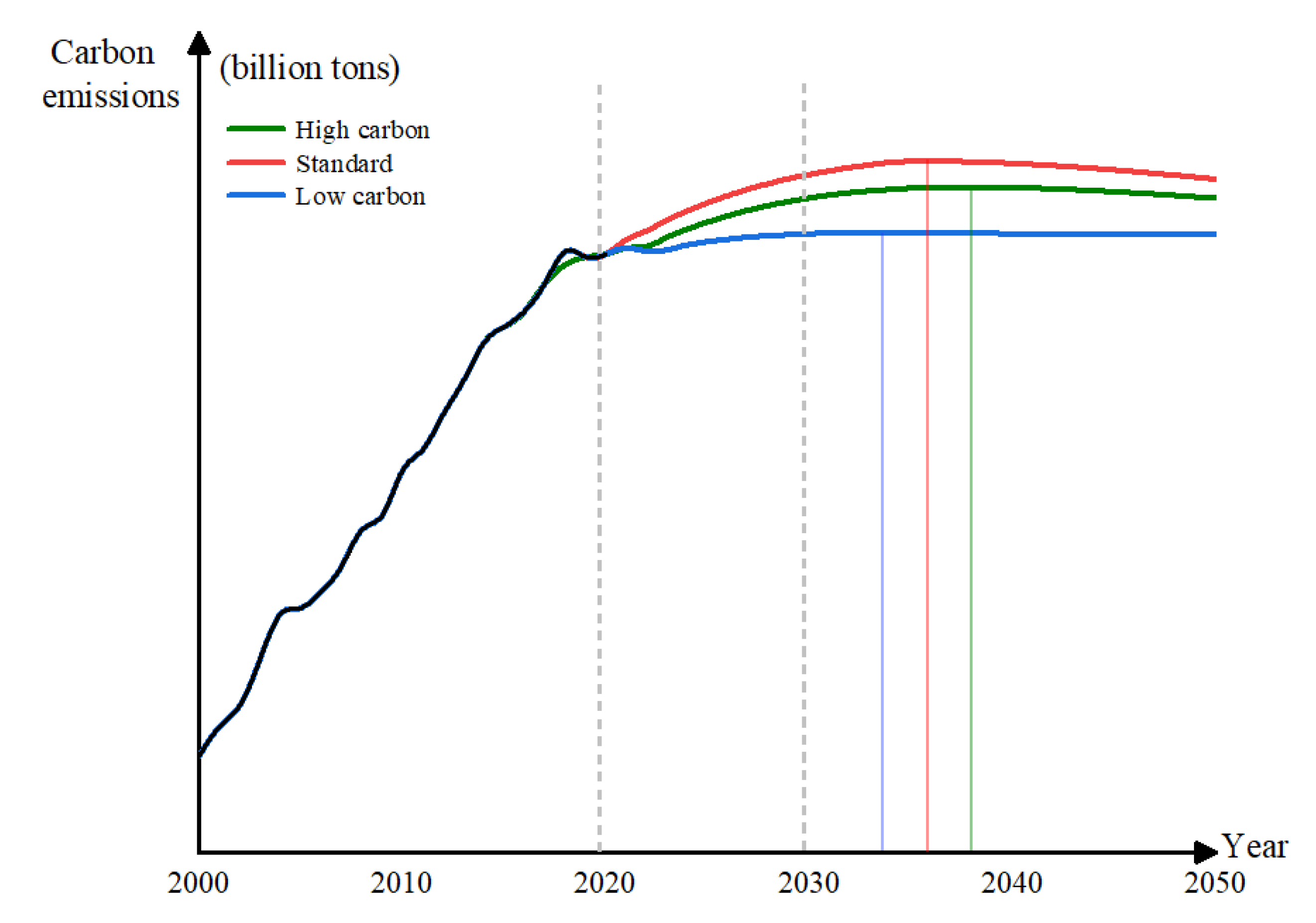
Based on the WOA-SVM model, the carbon emissions of the transportation industry in Jiangsu Province from 2022 to 2050 are predicted according to the different settings of the eight influencing factor indicators under the three scenarios of low carbon, baseline, and high carbon set in this study, and the prediction results are shown in Figure 7 and Table 8.
According to the study by Xiong [34] (p. 135894), The peak carbon year for China’s road transport sector will occur after 2030. Carbon emission trends under different scenarios are depicted, and time- and rate-based probabilities of achieving the peak carbon target are calculated. Miao [26] (p. 131417) believes that Jiangsu Province will most likely accomplish the peak carbon in 2025-2030. The study shows that the terminal energy intensity and the optimization of the energy industry structure are the most important means to achieve energy saving and carbon reduction.
Based on the prediction results of the WOA-SVM model in this study, the peak years of carbon emissions in the transportation industry in Jiangsu Province under the low-carbon, baseline, and high-carbon scenarios are 2034, 2036, and 2038, respectively. Under the high-carbon scenario, the peak is reached in 2036, with a peak of 50.60416 million tons. Under the baseline scenario, the peak is reached in 2038, with a peak of 48.71712 million tons. Under the low-carbon scenario, the peak is reached in 2034, with a peak of 45.37332 million tons. The high-carbon scenario has a higher overall annual growth rate during the peak and growth period and a lower overall annual decline rate during the decline period than the baseline scenario. The low-carbon scenario has a lower overall annual growth rate during the peak and growth period and a lower overall annual decline rate during the decline period than the baseline scenario.
6. Conclusion

This paper uses the WOA-SVM prediction model to simulate the carbon emission trends under three scenarios of Jiangsu Province’s transportation carbon emissions and predict the time of carbon peaking. An error comparison analysis is conducted on the LSTM, SVM, and GA-SVM prediction models to ensure the accuracy and scientific nature of the research results. The results show that the model in this study is significantly better than other prediction models in terms of error and correlation coefficient evaluation indicators, which improves the credibility of the prediction results. The results show that the carbon peak time in Jiangsu Province under the low-carbon scenario is 2034, which is closest to the official carbon peak target. Therefore, this paper proposes measures to promote low-carbon, efficient, and sustainable development of the transportation industry, such as policy guidance, optimization of the energy structure, and adjustment of the transportation structure, to achieve the carbon peak target as soon as possible.

Funding

This research received no external funding.

Institutional Review Board Statement

Not applicable.

Informed Consent Statement

Not applicable.

Data Availability Statement

Not applicable.

Conflicts of Interest

The authors declare no conflict of interest.

References

  1. Li, C.; Zhang, Z.; Wang, L. Carbon peak forecast and low carbon policy choice of transportation industry in China: Scenario prediction based on STIRPAT model. Environ. Sci. Pollut. Res. 2023, 30, 63250–63271. [Google Scholar] [CrossRef] [PubMed]
  2. Fan, F.; Lei, Y. Decomposition analysis of energy-related carbon emissions from the transportation sector in Beijing. Transp. Res. Part D Transp. Environ. 2016, 42, 135–145. [Google Scholar] [CrossRef] [PubMed]
  3. Xu, X.; Xu, H. The driving factors of carbon emissions in China’s transportation sector: A spatial analysis. Front. Energy Res. 2021, 9, 664046. [Google Scholar] [CrossRef]
  4. Rasool, Y.; Zaidi, S.A.H.; Zafar, M.W. Determinants of carbon emissions in Pakistan’s transport sector. Environ. Sci. Pollut. Res. 2019, 26, 22907–22921. [Google Scholar] [CrossRef] [PubMed]
  5. Ziyuan, C.; Yibo, Y.; Simayi, Z.; Shengtian, Y.; Abulimiti, M.; Yuqing, W. Carbon emissions index decomposition and carbon emissions prediction in Xinjiang from the perspective of population-related factors, based on the combination of STIRPAT model and neural network. Environ. Sci. Pollut. Res. 2022, 1–16. [Google Scholar] [CrossRef]
  6. Yin, F.; Bo, Z.; Yu, L.; Wang, J. Prediction of carbon dioxide emissions in China using a novel grey model with multi-parameter combination optimization. J. Clean. Prod. 2023, 404, 136889. [Google Scholar] [CrossRef]
  7. Wang, H.; Shi, W.; He, W.; Xue, H.; Zeng, W. Simulation of urban transport carbon dioxide emission reduction environment economic policy in China: An integrated approach using agent-based modelling and system dynamics. J. Clean. Prod. 2023, 392, 136221. [Google Scholar] [CrossRef]
  8. Modise, R.K.; Mpofu, K.; Adenuga, O.T. Energy and carbon emission efficiency prediction: Applications in future transport manufacturing. Energies 2021, 14, 8466. [Google Scholar] [CrossRef]
  9. Ning, L.; Pei, L.; Li, F. Forecast of China’s carbon emissions based on Arima method. Discret. Dyn. Nat. Soc. 2021, 2021, 1441942. [Google Scholar] [CrossRef]
  10. Zhou, W.; Lian, J.; Zhang, J.; Mei, Z.; Gao, Y.; Hui, G. Tomato storage quality predicting method based on portable electronic nose system combined with WOA-SVM model. J. Food Meas. Charact. 2023, 17, 3654–3664. [Google Scholar] [CrossRef]
  11. Ağbulut, Ü. Forecasting of transportation-related energy demand and CO2 emissions in Turkey with different machine learning algorithms. Sustain. Prod. Consum. 2022, 29, 141–157. [Google Scholar] [CrossRef]
  12. Mirjalili, S.; Lewis, A. The whale optimization algorithm. Adv. Eng. Softw. 2016, 95, 51–67. [Google Scholar] [CrossRef]
  13. Zhang, R.; Liu, M.; Pan, Z.; Yin, Y. Network security situation assessment based on improved WOA-SVM. Ieee Access 2022, 10, 96273–96283. [Google Scholar] [CrossRef]
  14. Cheng, Y.; Gai, X.; Jin, Y.; Guan, R.; Lu, M.; Ding, Y. A new method based on a WOA-optimized support vector machine to predict the tool wear. Int. J. Adv. Manuf. Technol. 2022, 121, 6439–6452. [Google Scholar] [CrossRef]
  15. Elkorany, A.S.; Marey, M.; Almustafa, K.M.; Elsharkawy, Z.F. Breast cancer diagnosis using support vector machines optimized by whale optimization and dragonfly algorithms. IEEE Access 2022, 10, 69688–69699. [Google Scholar] [CrossRef]
  16. Suthaharan, S.; Suthaharan, S. Support vector machine. Mach. Learn. Models Algorithms Big Data Classif. Think. Ex. Eff. Learn. 2016, 207–235. [Google Scholar]
  17. Mun, S.; Park, S.; Han, D.K.; Ko, H. Generative Adversarial Network Based Acoustic Scene Training Set Augmentation and Selection Using SVM Hyper-Plane. In Proceedings of DCASE; pp. 93–102.
  18. Wu, R.; Wang, J.; Wang, S.; Feng, K. The drivers of declining CO2 emissions trends in developed nations using an extended STIRPAT model: A historical and prospective analysis. Renew. Sustain. Energy Rev. 2021, 149, 111328. [Google Scholar] [CrossRef]
  19. Li, B.; Liu, X.; Li, Z. Using the STIRPAT model to explore the factors driving regional CO 2 emissions: A case of Tianjin, China. Nat. Hazards 2015, 76, 1667–1685. [Google Scholar] [CrossRef]
  20. Zhu, C.; Wang, M.; Du, W. Prediction on peak values of carbon dioxide emissions from the Chinese transportation industry based on the SVR model and scenario analysis. J. Adv. Transp. 2020, 2020, 8848149. [Google Scholar] [CrossRef]
  21. Zhu, C.; Yang, S.; Liu, P. Study on the factors influencing on the carbon emissions of Shaanxi Province’s transportation industry in China. Sustainability 2022, 14, 8610. [Google Scholar] [CrossRef]
  22. Xu, B.; Lin, B. Factors affecting carbon dioxide (CO2) emissions in China’s transport sector: A dynamic nonparametric additive regression model. J. Clean. Prod. 2015, 101, 311–322. [Google Scholar] [CrossRef]
  23. Niu, H.; Zhang, Z.; Xiao, Y.; Luo, M.; Chen, Y. A study of carbon emission efficiency in Chinese provinces based on a three-stage SBM-undesirable model and an LSTM model. Int. J. Environ. Res. Public Health 2022, 19, 5395. [Google Scholar] [CrossRef] [PubMed]
  24. Wang, P.; Wu, W.; Zhu, B.; Wei, Y. Examining the impact factors of energy-related CO2 emissions using the STIRPAT model in Guangdong Province, China. Appl. Energy 2013, 106, 65–71. [Google Scholar] [CrossRef]
  25. Eggleston, H.; Buendia, L.; Miwa, K.; Ngara, T.; Tanabe, K. 2006 IPCC guidelines for national greenhouse gas inventories. 2006.
  26. Miao, A.; Yuan, Y.; Wu, H.; Ma, X.; Shao, C.; Xiang, S. Pathway for China’s provincial carbon emission peak: A case study of the Jiangsu Province. Energy 2024, 298, 131417. [Google Scholar] [CrossRef]
  27. Liu, W.; Ren, Y.; Meng, X.; Tian, B.; Lv, X. Analysis of potential water inflow rates at an underground coal mine using a WOA-CNN-SVM approach. Water 2024, 16, 813. [Google Scholar] [CrossRef]
  28. Cong, Y.; Hou, L.; Wu, Y.; Ma, Y. Development of a Coupled EnergyPlus-MATLAB Simulation Based on LSTM for Predictive Control of HVAC System. Math. Probl. Eng. 2022, 2022, 5912967. [Google Scholar] [CrossRef]
  29. Xie, P.; Liao, J.; Pan, X.; Sun, F. Will China’s carbon intensity achieve its policy goals by 2030? Dynamic scenario analysis based on STIRPAT-PLS framework. Sci. Total Environ. 2022, 832, 155060. [Google Scholar] [CrossRef] [PubMed]
  30. Yi, X.; Jue, W.; Huan, H. Does economic development bring more livability? Evidence from Jiangsu Province, China. J. Clean. Prod. 2021, 293, 126187. [Google Scholar] [CrossRef]
  31. Lu, Q.; Chai, J.; Wang, S.; Zhang, Z.G.; Sun, X.C. Potential energy conservation and CO2 emissions reduction related to China’s road transportation. J. Clean. Prod. 2020, 245, 118892. [Google Scholar] [CrossRef]
  32. He, W.; Li, X.; Yang, J.; Ni, H.; Sang, X. How land use functions evolve in the process of rapid urbanization: Evidence from Jiangsu Province, China. J. Clean. Prod. 2022, 380, 134877. [Google Scholar] [CrossRef]
  33. Tang, D.; Ma, T.; Li, Z.; Tang, J.; Bethel, B.J. Trend prediction and decomposed driving factors of carbon emissions in Jiangsu Province during 2015–2020. Sustainability 2016, 8, 1018. [Google Scholar] [CrossRef]
  34. Xiong, S.; Yuan, Y.; Zhang, C. Achievement of carbon peak goals in China’s road transport—possibilities and pathways. J. Clean. Prod. 2023, 388, 135894. [Google Scholar] [CrossRef]
Figure 3. Total Carbon Emissions from Transport in Jiangsu Province in 2015.
Preprints 114443 g003
Figure 4. Total Carbon Emissions from Transport in Jiangsu Province in 2021.
Preprints 114443 g004
Figure 5. Training set error of WOA-SVM.
Preprints 114443 g005
Figure 6. Test set error of WOA-SVM.
Preprints 114443 g006
Figure 7. Future trends in carbon emissions from transportation under different scenarios.
Preprints 114443 g007
Table 1. Carbon emission factors for several common energy sources.
Energy type Average Low Calorific Value Carbon Content per Unit of Calorific Value Carbon Oxidation Rate Carbon Emission Factor
Unit KJ/kg or KJ/m³ Tg/TJ - kg-co2/kg
Raw Coal 20934 27.37 0.94 1.975
Gasoline 43134 18.90 0.98 2.929
Diesel fuel 42705 20.2 0.98 3.010
Natural gas 32238 15.32 0.99 1.793
Kerosene 43124 19.5 0.98 3.022
Fuel Oil 41868 21.1 0.98 3.174
Liquefied petroleum gas 50242 17.2 0.98 3.105
Electricity - - - 0.6451
Table 2. Selection of factors influencing transport carbon emissions in Jiangsu Province.
Serial Number Variant Unit (of Measure)
X1 Demographic all the people
X2 GDP per capita million dollars."
X3 Carbon intensity t-million-1
X4 Cargo turnover Billion tons-km-1
X5 Passenger turnover Billions of people-km-1
X6 Green space coverage in built-up areas %
X7 Urbanization rate %
X8 Personal vehicle ownership ten thousand vehicles
C Carbon footprint tons
Table 3. Carbon Emission Energy Consumption Data of Transportation Industry in Jiangsu Province.
Year X1 X2 X3 X4 X5 X6 X7 X8 X9 C
2000 7327.24 11765 74.51 107244 776.25 90436 1505.57 1.42 33.2 41.5
2001 7358.52 12879 87.12 110713 874.63 87505 1524.96 1.59 31.9 42.6
2002 7405.50 14369 705.50 115889 924.31 88588 1549.12 0.10 35.3 44.7
2003 7457.70 16743 778.61 123462 978.03 93511 1817.44 0.11 35.4 46.8
2004 7522.95 19790 872.82 128516 1109.19 100093 2398.64 0.12 37.9 48.2
2005 7588.24 23984 969.66 145204 1222.03 112909 3068.88 0.10 39.8 50.1
2006 7655.66 27868 1032.40 161425 1366.95 125114 3644.79 0.09 41.7 51.9
2007 7723.13 33798 1221.35 187241 1596.06 143805 4099.16 0.08 42.8 53.2
2008 7762.48 39967 1349.70 208237 1766.00 166322 4707.74 0.08 42.6 54.3
2009 7810.27 44272 1370.07 201262 1423.33 160967 5154.46 0.07 42.0 55.6
2010 7869.34 53525 1240.18 226627 1604.00 188558 6111.57 0.07 44.1 60.6
2011 8022.99 61464 1303.01 247405 1777.80 212594 7513.99 0.06 42.1 62.0
2012 8119.81 66533 1362.41 268371 1949.80 231295 8474.64 0.06 42.2 63.0
2013 8192.44 72768 1474.47 152172 1451.14 194048 10536.80 0.06 42.4 64.4
2014 8281.09 78711 1499.94 156016 1550.64 208623 11028.70 0.06 42.6 65.7
2015 8315.11 85871 1699.46 153943 1566.40 211648 7374.00 0.05 42.8 67.5
2016 8381.47 92658 1540.08 134605 1591.93 215651 8290.69 0.05 42.9 68.9
2017 8423.50 102202 1660.17 127952 1659.45 234092 9726.51 0.05 43.0 70.2
2018 8446.19 110508 1727.08 121884 1692.14 247388 9684.01 0.05 43.1 71.2
2019 8469.09 116650 1822.33 120802 1736.98 281060 11114.57 0.05 43.4 72.5
2020 8477.26 121333 1914.70 85164 1057.11 288513 11538.86 0.05 43.5 73.4
2021 8505.40 138255 2018.53 66156 1142.09 307176 12441.71 0.04 43.7 73.9
Table 4. Results of multiple covariance test.
Serial Number Variant VIF Value Tolerance Level
X1 Demographic 315.042 0.003
X2 GDP per capita 532.997 0.002
X3 Carbon intensity 10.753 0.093
X4 Cargo turnover 25.439 0.039
X5 Passenger turnover 11.656 0.233
X6 Green space coverage in built-up areas 22.752 0.044
X7 Urbanization rate 421.014 0.002
X8 Personal vehicle ownership 73.515 0.014
Table 5. Cumulative variance values of different principal components.
Implicit Variable One principal Component Two Principal Components Three Principal Components Four Principal Components
C 78.8 96.829 96.826 99.628
Table 6. Comparison of the results of the four prediction models.
Brochure Type of Error Algorithm Type
LSTM SVM GA-SVM WOA-SVM
Test set MAPE 0.1034 0.4249 0.0692 0.0549
RMSE 0.0480 0.2043 38.00e-4 33.00e-4
Table 8. Future projections of carbon emissions from transport under different scenarios.
particular year high carbon standard low carbon particular year high carbon standard low carbon
2022 4550.48 4435.1318 4360.1611 2037 5059.2705 4870.7817 4534.2773
2023 4627.6069 4501.9521 4411.2993 2038 5056.2471 4871.7124 4532.6792
2024 4695.8159 4561.4761 4445.7729 2039 5051.5488 4870.7988 4531.0161
2025 4755.9468 4614.1689 4469.7207 2040 5045.3521 4868.251 4529.3862
2026 4808.8213 4660.5039 4488.8018 2041 5037.8149 4864.2622 4527.8687
2027 4855.2178 4700.9448 4503.7275 2042 5029.0767 4859.0122 4526.52
2028 4895.8643 4735.9463 4515.1343 2043 5019.2627 4852.6655 4525.3862
2029 4931.4312 4765.9438 4523.5933 2044 5008.4814 4845.376 4524.4976
2030 4962.5283 4791.3511 4529.6084 2045 4996.8364 4837.2832 4523.8765
2031 4989.7026 4812.5605 4533.6245 2046 4984.4185 4828.5181 4523.5337
2032 5013.4438 4829.9429 4536.0322 2047 4971.3086 4819.1987 4523.4736
2033 5034.1855 4843.8413 4537.1709 2048 4957.584 4809.4346 4523.6958
2034 5052.3105 4854.584 4537.332 2049 4943.3149 4799.3252 4524.1943
2035 5059.4541 4862.4707 4536.7676 2050 4928.5679 4788.9619 4524.9595
2036 5060.4155 4867.7827 4535.6899 2051 4913.4028 4778.4287 4525.98
Disclaimer/Publisher’s Note: The statements, opinions and data contained in all publications are solely those of the individual author(s) and contributor(s) and not of MDPI and/or the editor(s). MDPI and/or the editor(s) disclaim responsibility for any injury to people or property resulting from any ideas, methods, instructions or products referred to in the content.
Copyright: This open access article is published under a Creative Commons CC BY 4.0 license, which permit the free download, distribution, and reuse, provided that the author and preprint are cited in any reuse.
Prerpints.org logo

Preprints.org is a free preprint server supported by MDPI in Basel, Switzerland.

Subscribe

© 2024 MDPI (Basel, Switzerland) unless otherwise stated