Research on SLAM Localization Algorithm for Orchard Dynamic Vision Based on YOLOD-SLAM2

With the development of agriculture, the complexity and dynamism of orchard environments pose challenges to the perception and positioning of inter row environments for agricultural machinery. The paper proposes a method for extracting navigation lines and measuring pedestrian obstacles. The improved YOLOv5 algorithm is used to detect tree trunks between left and right rows in orchards. The experimental results show that the average angle deviation of the extracted navigation lines is less than 5 degrees, verifying its accuracy. Due to the variable posture of pedestrians and ineffective camera depth, a distance measurement algorithm based on four zone depth comparison is proposed for pedestrian obstacle distance measurement. Experimental results show that within a range of 6m, the average relative error of distance measurement does not exceed 1%, and within a range of 9m, the maximum relative error is 2.03%. The average distance measurement time is 30 milliseconds, which can accurately and quickly achieve pedestrian distance measurement in orchard environments. On the publicly available TUM RGB-D dynamic dataset, YOLOD-SLAM2 significantly reduces the RMSE index of absolute trajectory error compared to ORB-SLAM2 algorithm, which is less than 0.05 m/s. In actual orchard environments, YOLOD-SLAM2 has a higher degree of agreement between the estimated trajectory and the true trajectory when the car is traveling in straight and circular directions. The RMSE index of the absolute trajectory error is less than 0.03m/s, and the average tracking time is 47ms, indicating that the YOLOD-SLAM2 algorithm proposed in this paper can meet the accuracy and real-time requirements of agricultural machinery positioning in orchard environments.

Keywords:

Subject: Engineering - Other

1. Introduction

In recent years, the fruit tree industry has experienced rapid development worldwide. The autonomous navigation technology of unmanned agricultural machinery in orchards has been an important topic of concern in the agricultural field in recent years [1,2]. During autonomous operation of agricultural machinery, obstacles such as pedestrians may be encountered, and real-time detection and distance measurement of obstacles are required to provide information for subsequent obstacle avoidance, thereby improving the safety and reliability of autonomous operation of agricultural machinery [3]. The orchard environment is complex and ever-changing, with high real-time requirements. How to quickly and accurately detect obstacles has become a research focus. Traditional orchard robot navigation technology mainly relies on Global Navigation Satellite System (GNSS) and Inertial Measurement Unit (IMU) [4]. However, when working between rows of fruit trees, GNSS often cannot provide sufficient positioning accuracy due to factors such as tree obstruction. When using IMU for positioning, accumulated errors will occur over time, and there are also problems of zero bias and temperature drift [5]. Therefore, visual navigation technology has become an important navigation tool for orchard robots.

In the orchard environment, inter row navigation line extraction refers to using sensors to obtain orchard environment information, and then analyzing and processing it through algorithms to extract navigation lines that can be used for autonomous navigation of agricultural machinery. Common sensors include LiDAR and visual sensors. With the development of computer vision and deep learning technologies, some researchers have begun to explore the use of traditional methods such as K-Means clustering and OTSU threshold segmentation [6,7], as well as deep learning methods such as semantic segmentation and object detection, to extract navigation lines. Radcliffe J et al. used the similarity between the shape of the sky in orchard images and the shape of the ground constrained by tree trunks to extract the path plane through the green component and calculate the centroid of the path plane to determine the heading of the navigation path, taking advantage of the large difference between the crown of fruit trees and the sky background [8]. OPIYO S et al. proposed a machine vision technique based on the intermediate axis to extract orchard navigation lines. This method first converts the RGB image into a grayscale image and extracts texture features. Then, the K-Means clustering method is used to obtain binary images, and finally the middle axis is used as the navigation line [9].

In terms of research on obstacle detection methods, Bochkovskiy A et al. proposed YOLOv4, a technique for enhancing Mosaic image data [10]. This method utilizes Path Aggregation Network (PANet) [11] for multi-scale feature fusion and adopts CIOU loss (Cross Intersection over Union Loss) as the position loss function for prediction boxes [12], significantly improving detection speed and accuracy. The YOLOv5 proposed by Ultralytics et al. is an improved and optimized single-stage object detection algorithm based on YOLOv3 [13]. It modularizes the network structure and proposes a new training strategy that can quickly and accurately detect targets. Hsu W Y et al. proposed a pedestrian detection method based on multi-scale adaptive fusion to address the uncertainty and diversity of pedestrians under different scales and occlusion conditions. The method designed a segmentation function to achieve segmentation of non overlapping pedestrian areas in the input image and obtain sub images. Then, a multi-resolution adaptive fusion method was proposed to fuse all sub images with the input image, improving the model’s ability to detect pedestrians of different scales [14]. Wan et al. proposed an STPH-YOLOv5 algorithm to address the problem of slow detection speed and low detection accuracy caused by pedestrian occlusion and pose changes in dense pedestrian detection. The algorithm uses a layered visual Transformer prediction head (STPH) and coordinate attention mechanism, and uses a weighted bidirectional feature pyramid (BiFPN) in the Neck section to improve sensitivity to targets of different scales and enhance the overall detection capability of the model [15].Panigrahi S et al. proposed an improved YOLOv5 method, which improves the Darknet19 backbone network and introduces separable convolution and Inception deep convolution modules, aiming to improve model performance with minimal overhead [16].

In terms of research on visual SLAM localization methods, Wang R et al. used basic matrices to detect feature point inconsistencies and cluster depth images, achieving segmentation of moving objects and removing feature points on moving objects [17]. Cheng J et al. proposed a Sparse Motion Removal (SMR) model. This model is based on the Bayesian framework and detects dynamic regions based on the similarity between consecutive frames and the difference between the current frame and the reference frame [18]. Sun Y et al. proposed a visual SLAM algorithm based on RGB-D information for real-time removal of dynamic foreground targets. Due to the use of dense optical flow for tracking, this algorithm is limited and time-consuming in high-speed scenes. As the optical flow method degrades, its segmentation accuracy for dynamic targets also decreases [19]. Liu G et al. proposed a DMS-SLAM algorithm. This algorithm combines GMS feature matching algorithm and sliding window to construct static initialization map points. Based on the GMS feature matching algorithm and the map point selection method between keyframes, static map points are added to the local map to create a static 3D map that can be used for attitude tracking. However, it is prone to failure when the dynamic target is too large [20]. G. Li et al. used a small number of feature points to detect moving objects based on epipolar geometric constraints, obtained dynamic feature points, and then obtained dynamic Region of Interest (RoI) regions based on disparity constraints using dynamic feature points. They used an improved SLIC superpixel segmentation algorithm to segment the dynamic RoI regions and obtain dynamic target regions [21]. Yu C et al. proposed the DS-SLAM algorithm [22], which utilizes the semantic segmentation network SegNet to segment images and integrates optical flow estimation to distinguish between static and dynamic objects in the environment [23]. However, it has a high computational cost and poor real-time performance. Bescos B et al. [24] proposed a DynaSLAM algorithm that combines Mask R-CNN [25] and multi view geometry to perform pixel segmentation on dynamic objects, obtain dynamic regions, and then remove feature points from the dynamic regions.

By analyzing the current research status of navigation line extraction, obstacle detection, and dynamic visual SLAM positioning methods at home and abroad, this paper aims to use binocular vision and deep learning technology to study the perception and positioning methods of agricultural machinery environment suitable for orchard environment, and to research high-precision and robust algorithms for agricultural machinery orchard environment perception and positioning, providing strong support for the automation and intelligence of orchard operations.

2. Materials and Methods

2.1. Camera Model and Parameter Calibration

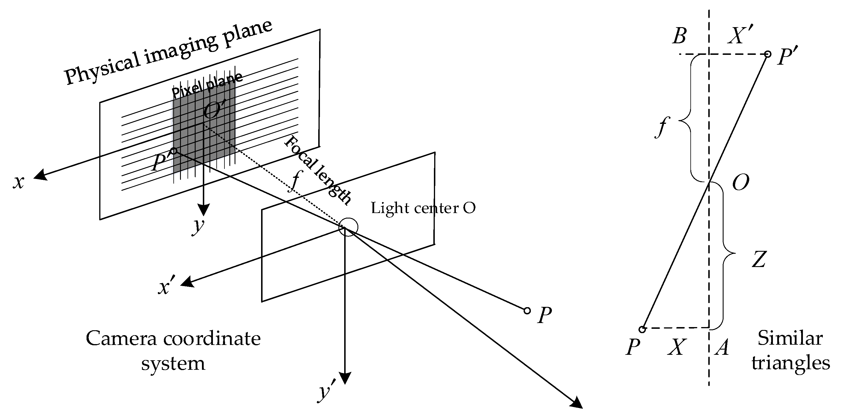
The paper uses the ZED2i binocular camera for visual research on orchard environments, as shown in Figure 1. The ZED2i camera adopts a pinhole camera model, which optimizes outdoor shooting conditions and improves image color depth and quality through dual 4mm lenses and polarizing filters. The camera spacing is 12cm, supporting a maximum depth measurement of 40m, with an error of no more than 1m within a 10m range. Its maximum viewing angle is 110 °, suitable for visual capture of wide scenes. The depth image is obtained by calculating the disparity through stereo matching of binocular images, and deriving depth information using internal and external parameters to ensure accurate depth measurement and visual perception.

Assuming there is a point

P = {[X, Y, Z]}^{T}

in the three-dimensional space, the point

P^{'} = {[X^{'}, Y^{'}, Z^{'}]}^{T}

is obtained by projecting the small hole O onto the camera imaging plane, and the camera focal length f is the distance from the imaging plane to the small hole O. According to the triangle similarity relationship, in practice, the camera produces a positive image, and the following formula can be obtained through the symmetry relationship:

{\begin{matrix} X^{'} = f \frac{X}{Z} \\ Y^{'} = f \frac{Y}{Z} \end{matrix}

(1)

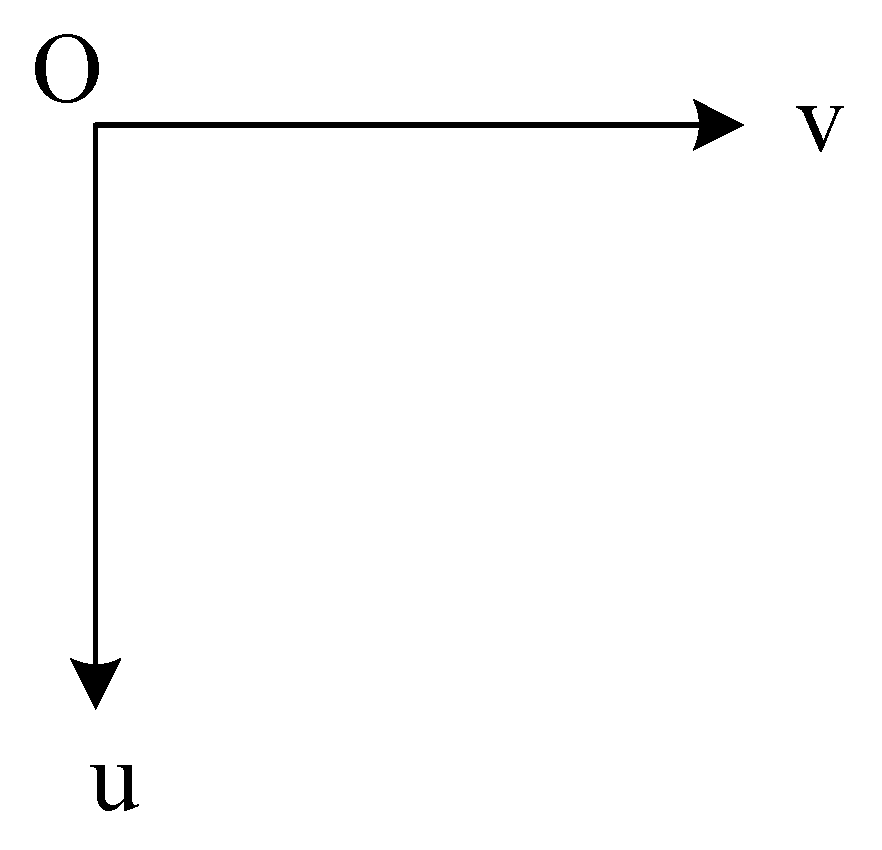
The structure of the pixel coordinate system is shown in Figure 2. In the pixel coordinate system, the origin

O^{'}

is located in the upper left corner of the image, with the horizontal axis to the right as the horizontal axis, which is the u axis, and the vertical axis from top to bottom, which is the v axis. In the pixel coordinate system, relative to the camera imaging plane, assuming that each pixel coordinate is scaled

α

times on the u axis and

β

times on the v axis, and

O^{'}

is shifted

{[c_{x}, c_{y}]}^{T}

relative to O, the following derivation can be obtained:

{\begin{cases} u = α X^{'} + c_{x} \\ v = β Y^{'} + c_{y} \end{cases}

(2)

According to equations (1) and (2), let

f_{x} = α f, f_{y} = β f

(3)

In summary, the following formula can be obtained，

Z (\begin{array}{l} u \\ v \\ 1 \end{array}) = (\begin{matrix} f_{x} & 0 & c_{x} \\ 0 & f_{y} & c_{y} \\ 0 & 0 & 1 \end{matrix}) (\begin{array}{l} X \\ Y \\ Z \end{array}) \overset{d e f}{=} K P

(4)

where, K is the camera’s internal parameter matrix. For the camera’s external parameters, they are determined by the camera’s motion and can be described by the camera’s rotation matrix R and displacement vector t. Where T is the camera’s external parameter matrix, as shown in the equation, T can be expressed as:

Z P_{u v} = Z (\begin{array}{l} u \\ v \\ 1 \end{array}) = K (R P_{w} + t) = K T P_{w}

(5)

2.2. YOLOv5 Object Detection Algorithm and ORB-SLAM2 Algorithm

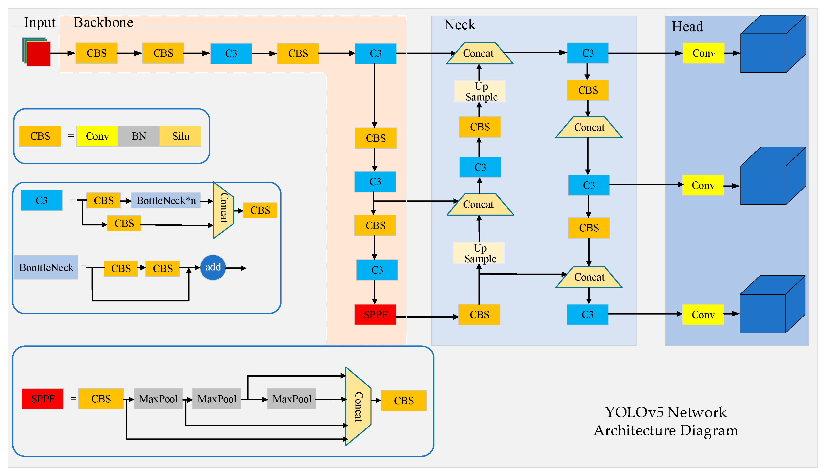
The paper is based on the YOLOv5s object detection model for improvement, which includes input, Backbone, Neck, and Head parts. The YOLOv5s network structure is shown in Figure 3. Firstly, the input image is divided into S × S grids, and feature extraction is performed through Backbone. Feature fusion is performed in the Neck section, and different scale feature maps are predicted in the Prediction section. Redundant boxes are filtered out according to NMS to achieve target detection.

The ORB-SLAM2 algorithm is one of the mainstream visual SLAM algorithms, suitable for ORBSLAM2, which is a real-time system based on vision for simultaneous localization and mapping. It is suitable for cameras including monocular, binocular, and RGB-D cameras, and can achieve relative localization based on visual information, namely camera pose estimation and optimization. The ORB-SLAM2 algorithm typically runs at 10-30 frames per second and can operate stably in static indoor environments. However, for outdoor environments, it is affected by lighting and uncertain dynamic targets, resulting in positioning accuracy that deviates from reality and requires improvement.

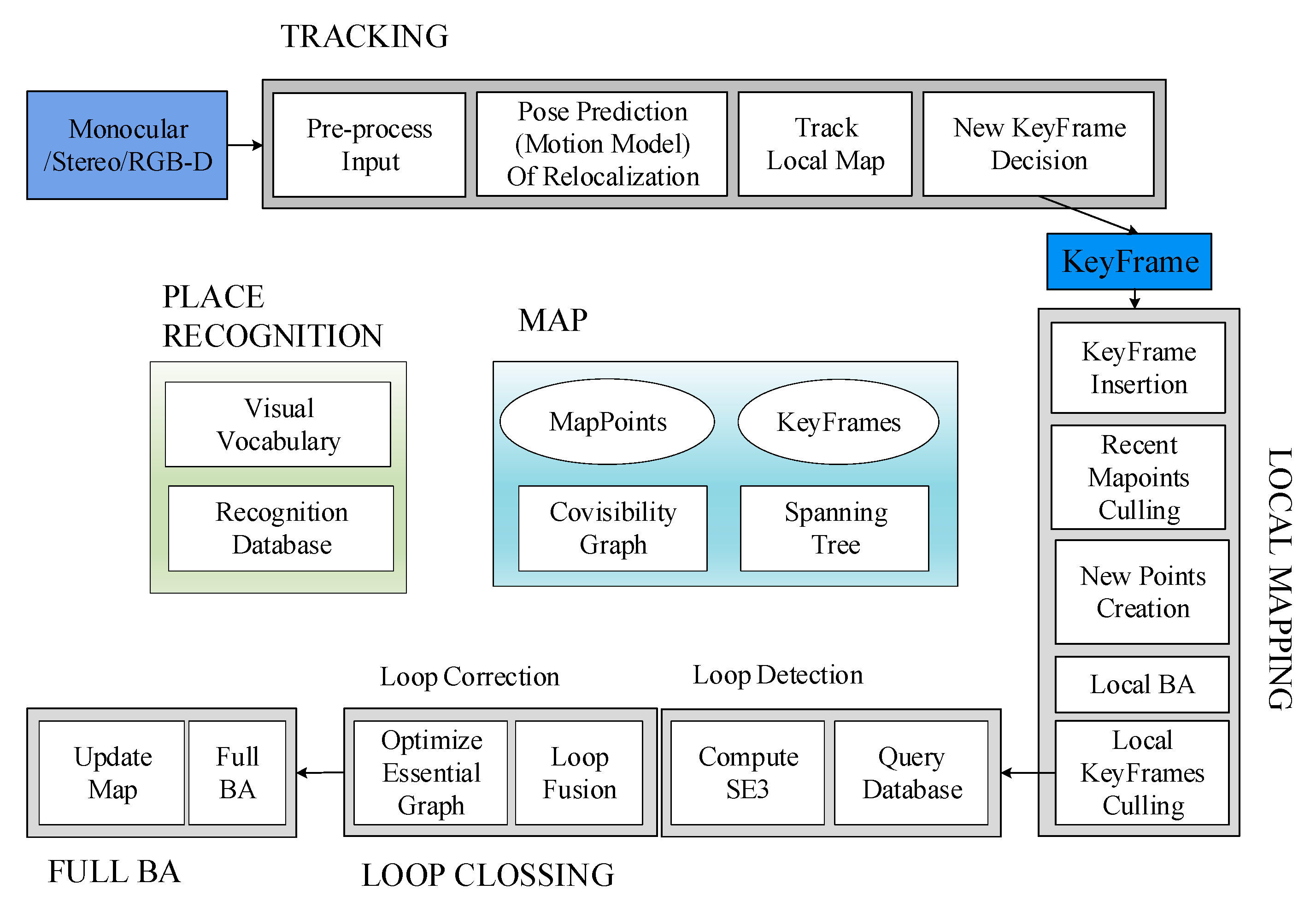
The ORB-SLAM2 principle diagram is shown in Figure 4, which includes three main threads: the Track tracking thread, the Local Mapping thread for local mapping, and the Loop Closing thread for closed-loop detection. And the fourth thread is Full BA, which bundles and adjusts the optimized pose.

3. Results and Discussion

3.1. Navigation Line Extraction and Experimental Verification

3.1.1. Test Method

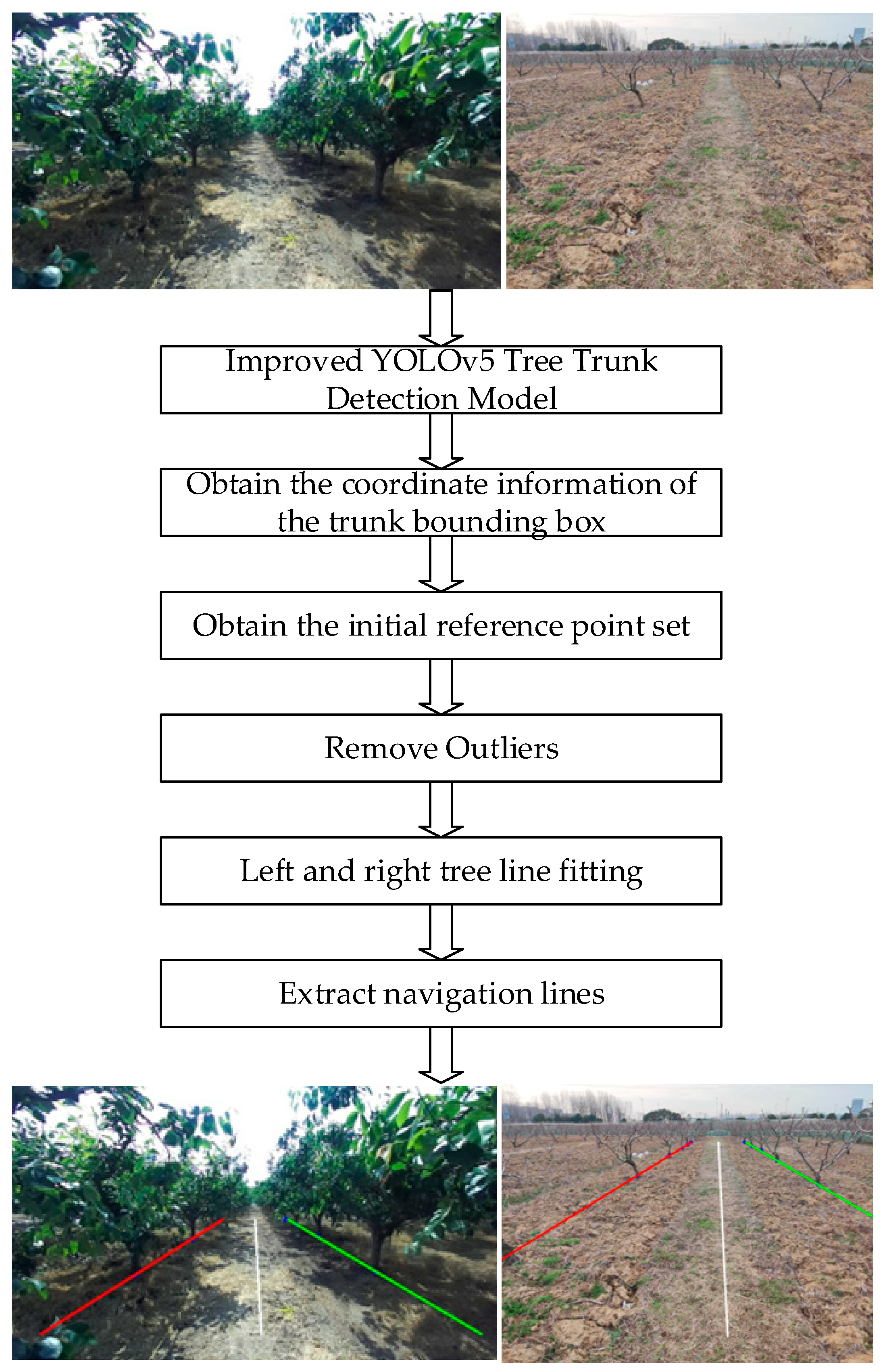
The paper is based on an improved YOLOv5 convolutional neural network as the initial detection, and studies the methods of extracting inter row navigation lines and obstacle ranging in orchards. In the orchard, the navigation line provides heading information for the autonomous operation of agricultural machinery. In the orchard, it is a straight line, and the extraction process is shown in Figure 5.

For the extraction of navigation lines between orchard rows, the paper uses an improved YOLOv5 convolutional neural network for tree trunk detection, obtaining the coordinate information of the detection bounding box of the tree trunk. Based on the detection bounding box, the left and right initial reference point sets are calculated separately. By improving RANSAC to screen the initial reference point set and removing outliers, the left and right reference point sets are obtained. Then, the left and right point sets are fitted with least squares to obtain the left and right tree lines, and the navigation lines are extracted.

Figure 5. Algorithm flowchart.

The paper is based on the improved YOLOv5 trained on a dataset of tree trunks and pedestrians in an orchard, and obtains a tree trunk detection model to obtain the detection bounding box coordinate information (cx, cy, w, h) of the tree trunk. In a real orchard environment, the root point of the tree trunk can be used as a reference point to fit the tree line.

Due to different orchard environments and perspectives, not all available reference points can be used as reference points for tree line fitting. The specific problem can be described as the following two situations.

As shown in Figure 6, within the field of view of the image, there are too few tree trunks that can be detected on one side, resulting in a large deviation when performing line fitting. It is necessary to preserve the initial reference point as much as possible.

As shown in Figure 7, reference points are also obtained in adjacent tree rows, which are interference points that will affect the subsequent tree row line fitting. It is necessary to remove the interference points.

In response to the above issues, this section uses the RANSAC (Random Sample Consensus) algorithm to distinguish between inliers and outliers for different detection scenarios, remove outliers, and obtain a reference point set.

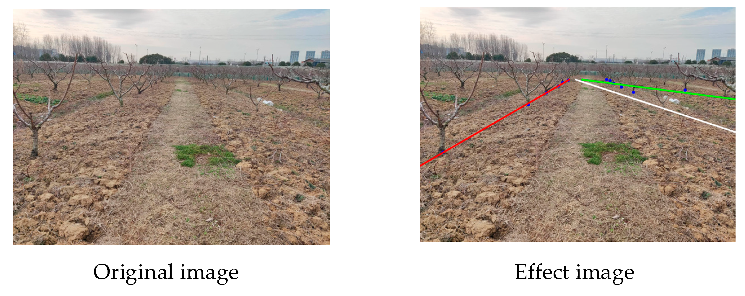
The rows of fruit trees are generally a straight line, and the least squares fitting algorithm is commonly used to fit the line. Its basic idea is to find a straight line that minimizes the distance between all data points and that line. For the straight line model on a two-dimensional plane, the outlier points in the reference point set were removed by combining RANSAC. Based on the reference point set, the least squares fitting was performed to obtain the left and right rows, and the navigation lines were extracted as shown in Figure 8. The red line is the left row line between fruit tree rows, the green line is the right row line, and the white line is the extracted navigation line.

3.1.2. Result Analysis

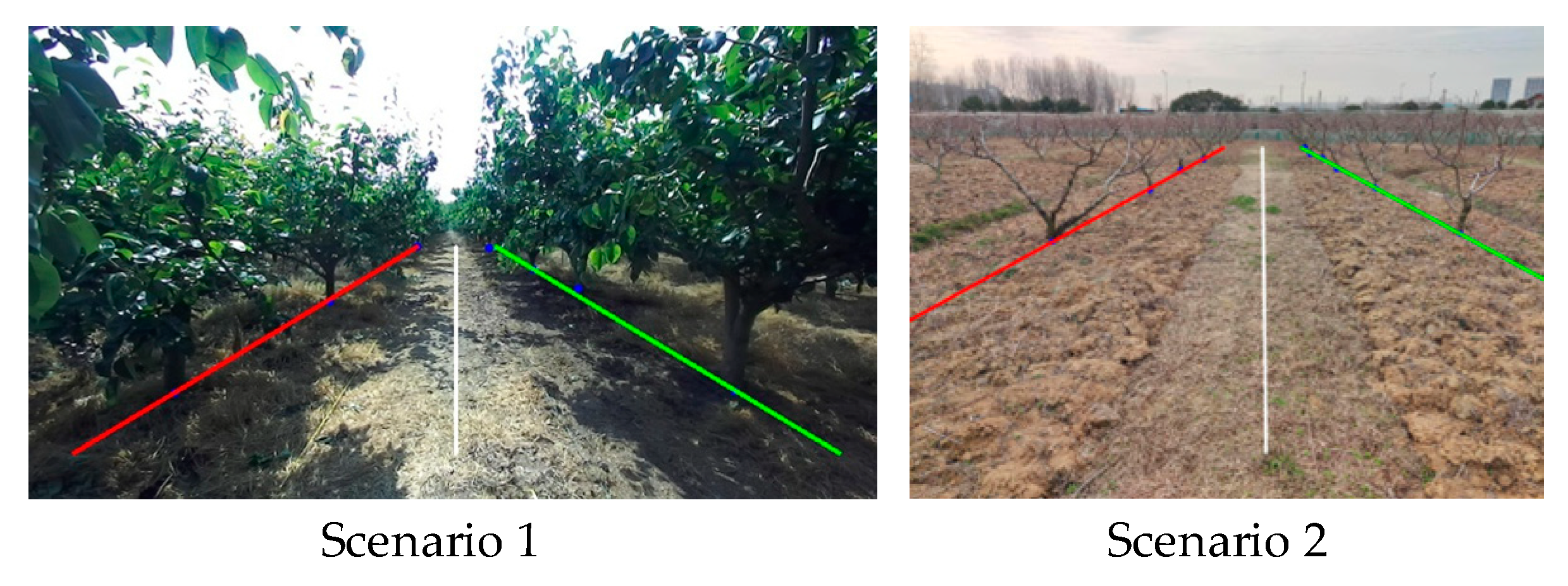
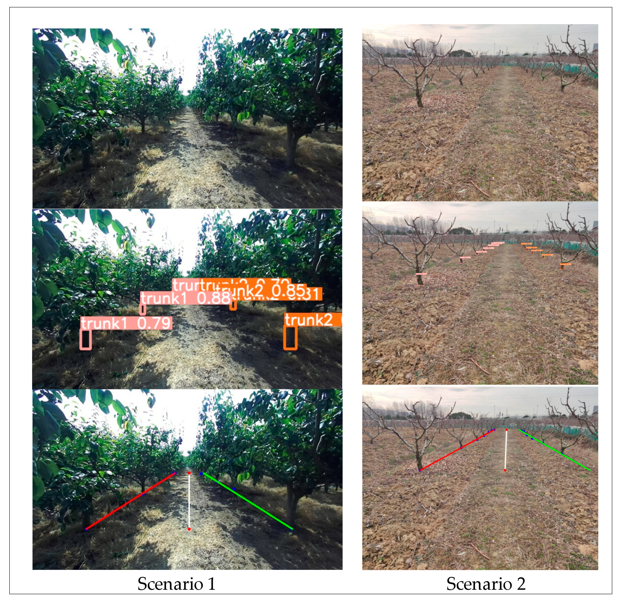
The paper uses an optimized YOLOv5 convolutional neural network model for tree trunk detection. After obtaining the coordinates of the tree trunk bounding box, the initial reference point set is calculated. Considering that the tree rows and navigation lines in the orchard are approximately straight lines, the paper adopts outlier removal and line fitting methods to improve the robustness of the algorithm. As shown in Figure 9, the red line represents the left tree line, the green line represents the right tree line, the white line represents the navigation line, and the blue point represents the tree line fitting reference point. The experimental results show the effectiveness of navigation line extraction in different orchard scenes, including the original image, tree trunk detection result image, and navigation line extraction result image in sequence.

According to the results in the above figure, it can be seen that the detection results of tree trunks are relatively correct in different scenarios of the orchard. After removing outliers and fitting tree lines, the extracted navigation lines highly match the actual scene. The experimental results demonstrate the effectiveness and accuracy of the algorithm proposed in this section.

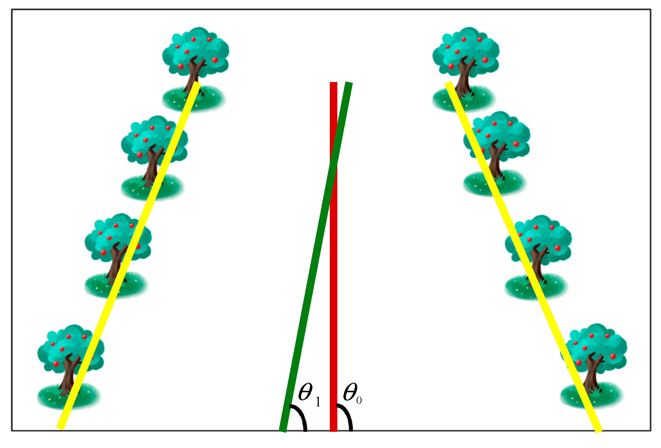
The paper uses fitted navigation lines and manually annotated navigation lines for error calculation. The angle between the navigation line and the horizontal direction of the image is the angle of the navigation line, denoted as θ, with a value range of [0,90]. In the rows of the orchard, the agricultural machinery travels forward in a straight line, and the indicator evaluation diagram is shown in Figure 10.

In order to analyze the error between the navigation lines extracted by the algorithm in this section and the manually annotated navigation lines, the paper randomly selected 100 images from two different scenarios in the orchard as the test set. Based on the previous indicators, statistical results of angle deviation and lateral deviation were obtained, as shown in Figure 11, and the average angle deviation and angle standard deviation were calculated. From Figure 11, it can be seen that the maximum deviation of the angle in Scene 1 is 7.5446 °, and the maximum deviation of the angle in Scene 2 is 18 °. Most of the angle deviations are below 6 °. The corresponding results show that the algorithm proposed in the paper can meet the accuracy requirements of navigation in orchards.

As shown in Table 1, in scenario 1, the average angle deviation of the extracted navigation line is 1.4797 °, and the standard deviation of the angle deviation is 1.3675 °, indicating a small error. For scenario 2, the average angle deviation is 2.8942 °, and the standard deviation of the angle deviation is 2.7102 °, which is twice the error compared to scenario 1. The reason is that the perspective of the images collected in Scene 2 is variable, which causes the algorithm to be unstable, but the error value still meets the accuracy requirements for navigation line extraction, that is, this algorithm can adapt to navigation line extraction in two different scenes.

When analyzing the extraction speed of navigation lines, input a test set of images from different scenes in the orchard. Set the time in the processing script, record the algorithm processing time, count the processing time of each sample, and calculate the average value as the average extraction time of the algorithm, as shown in Table 2. In two different scenarios, the average extraction time of the algorithm is 47.98ms and 56.11ms, respectively, which proves that it meets the real-time requirements for extracting navigation routes in the orchard.

3.2. Pedestrian Distance Measurement Method and Experiment Based on Four Zone Depth Comparison

3.2.1. Test Method

The traditional method for target distance measurement usually uses the detection of the center of the bounding box to calculate the distance of the target. However, due to the different postures of pedestrians, the center point of the pedestrian detection bounding box cannot correspond to the center point of the pedestrian target, thereby reducing the accuracy and precision of distance measurement based on the detection bounding box center point for pedestrians.

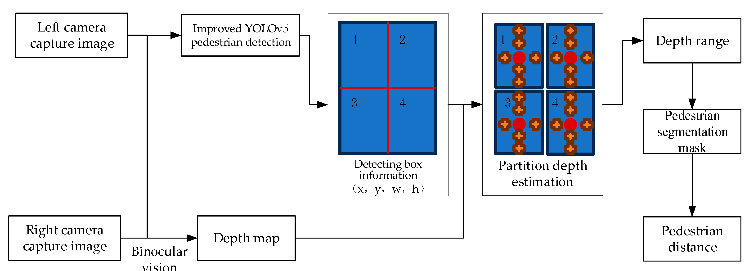
As shown in Figure 12, the paper proposes a pedestrian ranging algorithm based on four zone depth comparison. By dividing the detection bounding box into 2 * 2, i.e. 4 zones, the minimum depth is calculated for each zone and compared. Then, the approximate minimum depth of pedestrians is obtained, and the depth range of pedestrians is obtained to achieve segmentation of pedestrians. The average depth within the pedestrian mask range is calculated to obtain the distance of pedestrians.

Based on the improved YOLOv5 convolutional neural network as shown in Figure 12, the image of the left camera is detected. If a pedestrian is detected, the coordinate information of the pedestrian detection box is obtained as (x, y, w, h), and the pixel coordinates are restored according to the size of the image (pW, pH).

X = x * p W, Y = y * p H, W = w * p W, H = h * p H

respectively represent the pixel coordinates (X, Y) of the center point of the detection bounding box, as well as the width W and height H of the erasure bounding box;

Then, based on binocular vision, a depth map is obtained from the left and right images. The detection box is divided into four partitions: top, bottom, left, and right. Depth statistics are performed on each partition. For each partition, the average depth values from the upper center point to the regional center point (red point in the figure), from the local center point to the regional center point, from the left center point to the regional center point, and from the right center point to the regional center point are

D_{t}^{i}, D_{b}^{i}, D_{l}^{i}, D_{r}^{i}, i = (1, 2, 3, 4)

, representing the four partitions respectively. Compare the average depth values extracted from the left and right sides of the center point, sort all depth values on the smaller side, take the top 5 minimum depth values, and calculate their average. Apply the same treatment to the depth values at the top and bottom, and calculate the average value.

Compare the above two means and take the depth with the smaller mean as the approximate minimum depth for the partition; Finally, the approximate minimum depth of the four partitions is sorted, and the minimum depth is selected as the pedestrian depth Dperson. The depth range is defined as [DPerson -0.2, Dperson+0.2]. Based on the depth range, the average depth within the detection box is calculated to obtain the pedestrian distance. The calculation formulas are represented as follows.

{\begin{cases} D_{t b}^{i} = \min (D_{t}^{i}, D_{b}^{i}) \\ D_{l r}^{i} = \min (D_{l}^{i}, D_{r}^{i}) \end{cases}

(6)

{\begin{cases} s o r t e d (D_{t b}^{i}), s o r t e d (D_{l r}^{i}) \\ D^{i} = (\sum_{t = 1}^{5} \min (D_{t b}^{i}, D_{l r}^{i})) / 5 \end{cases}

(7)

D p e r s o n = \min (D^{1}, D^{2}, D^{3}, D^{4})

(8)

D r a n g e = [D p e r s o n - 0.2, D p e r s o n + 0.2]

(9)

3.2.2. Result Analysis

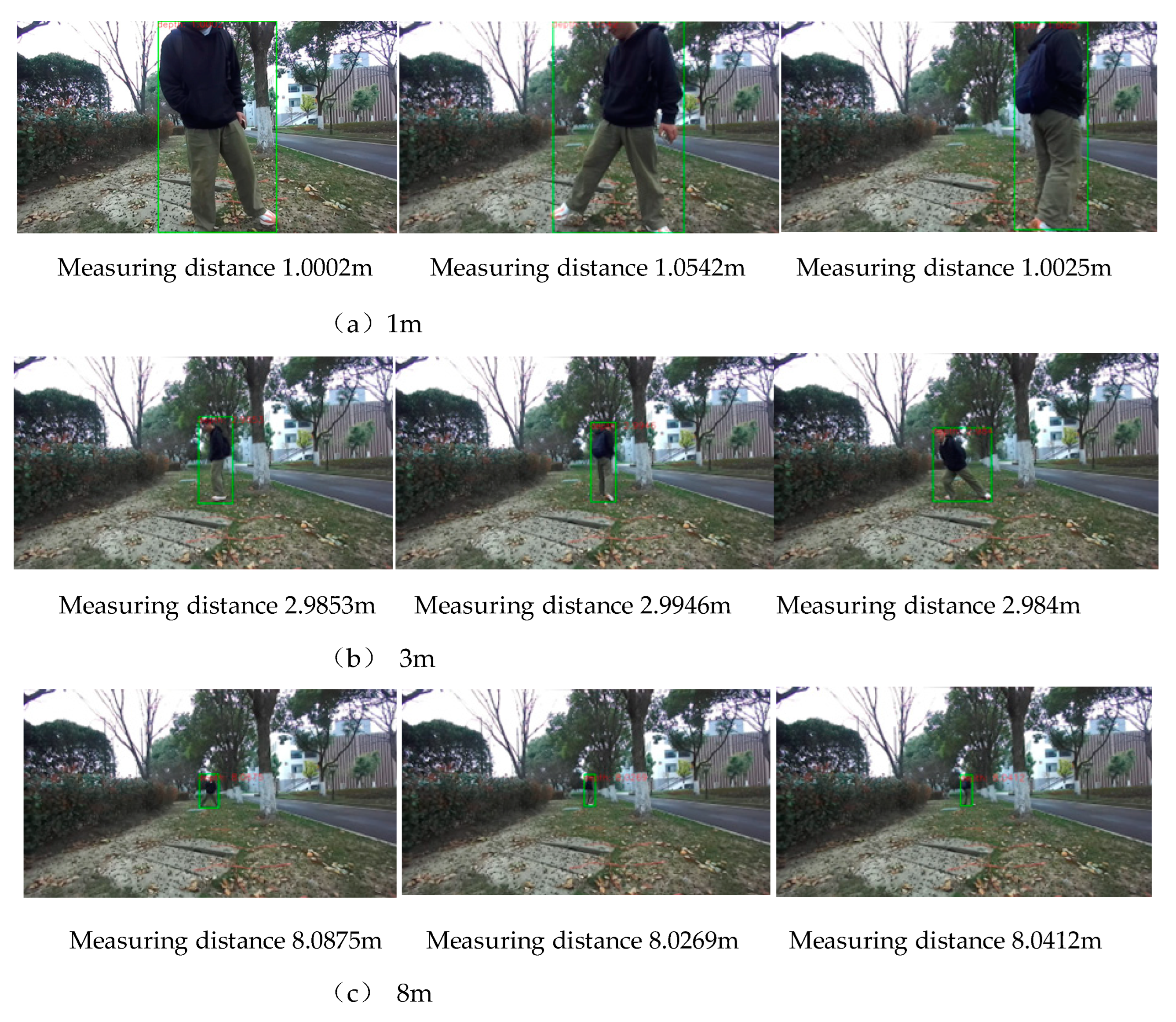
The paper conducts data measurement experiments using a ZED2i binocular camera. The camera is fixed on a mobile device, and in a simulated orchard environment, the mobile device moves at a constant speed. The camera’s field of view is in front of pedestrians, who remain stationary at fixed positions, as shown in Figure 13. The algorithm proposed in the paper visualizes the results at 1m, 3m, and 8m, with three images in each row representing the distance measurement results under three different pedestrian postures, where the distance measurement unit is meters (m).

The experimental results show that within the optimal range of the binocular camera, at a distance of 1m, the algorithm measures distances of 1.0002m, 1.0542m, and 1.0025m for pedestrians in three different postures; At a distance of 3m, the distances are 2.9853m, 2.9946m, and 2.984m, respectively. The maximum distance error is about 5cm, and the average error is 1.55cm, indicating that the algorithm has high accuracy and verifying its accuracy. When exceeding the optimal range of the camera, at a distance of 8m and in different poses, the algorithm measures distances of 8.0875m, 8.0269m, and 8.0412m, respectively, with a maximum error of about 8cm, which is relatively large. The main reason for the large error is that the binocular camera has fewer effective depth points as the distance increases, resulting in inaccurate ranging. However, in actual orchard scenes, the effective distance for obstacle detection is generally between 1m-6m, which proves that this algorithm meets the requirements of orchard obstacle ranging.

In order to verify the accuracy of distance measurement, the paper obtains the true value of pedestrian distance through laser radar. Comparative experiments are conducted on the pedestrian distance measurement algorithm based on center point distance measurement and the four zone depth comparison proposed in the paper, and error analysis is carried out with the true value to prove the feasibility and accuracy of the proposed algorithm. The experimental results are shown in Table 3.

Table 3. Distance measurement based on center point.

No.	Actual distance/m	Calculated distance/m	Relative error/（m）
1	1.0	0.961	3.90%
2	1.5	1.458	2.80%
3	2.0	1.98	1.00%
4	3.0	2.957	1.43%
5	4.0	3.986	0.35%
6	6.0	6.081	1.35%
7	8.0	8.164	2.05%
8	9.0	9.267	2.97%
9	10.0	10.294	2.94%

Table 4. Distance measurement based on four zone depth comparison.

No.	Actual distance/m	Calculated distance/m	Relative error/（m）
1	1.0	1.0031	0.318%
2	1.5	1.5088	0.587%
3	2.0	2.0097	0.485%
4	3.0	2.9987	0.043%
5	4.0	4.0082	0.205%
6	6.0	6.0225	0.375%
7	8.0	8.0875	1.094%
8	9.0	9.1156	1.284%
9	10.0	9.7966	2.034%

From Table 3 and Table 4, it can be seen that the pedestrian distance measurement algorithm proposed in the paper has a relative error of no more than 1% within 6 meters and a high distance measurement accuracy. After exceeding 6m, the error begins to increase, showing a gradually increasing trend, but the overall error is also within 3%. When pedestrians are 10m away from the camera, the error reaches 2.034%. Therefore, the algorithm proposed in the paper achieves distance measurement by calculating the average depth of pedestrians within a depth range, which can effectively represent the overall distance of pedestrians. It is less affected by pedestrian posture and background, and its accuracy has been significantly improved.

3.3. Localization Method Based on YOLOD-SLAM2

3.3.1. Test Method

The paper proposes a YOLOD-SLAM2 localization algorithm that combines YOLOv5, binocular depth information, and ORB-SLAM2. Through YOLOv5 and depth information, pedestrian segmentation is achieved to obtain semantic information of dynamic pedestrian targets. This information is then fused with ORB-SLAM2 to eliminate dynamic feature points and improve its localization accuracy.

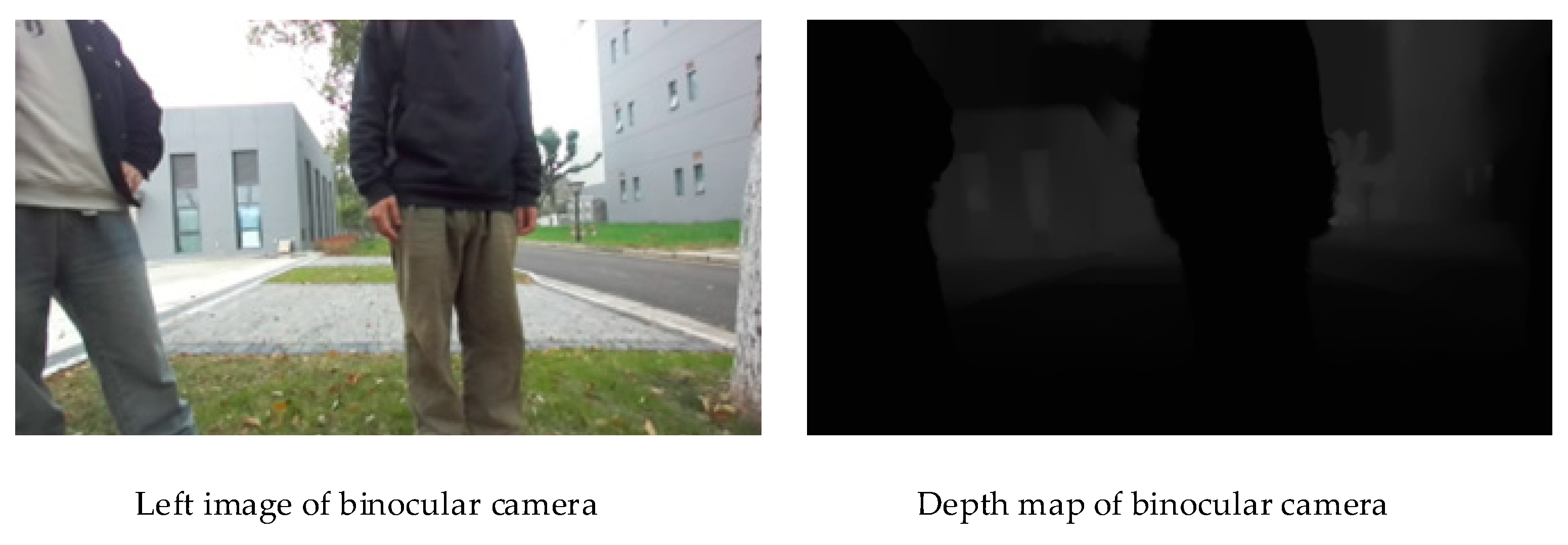
As shown in Figure 14, the paper combines YOLOv5 object detection and ORB-SLAM2 in the dynamic vision SLAM algorithm to optimize real-time performance and localization accuracy. YOLOv5 is used to detect pedestrians and extract their semantic information, which is then passed on to ORB-SLAM2 to help remove dynamic feature points. the paper proposes a pedestrian semantic information acquisition strategy based on depth information, taking into account the characteristics of the human body as a non rigid structure. By introducing a distance measurement algorithm based on four zone depth comparison, the approximate minimum depth of dynamic targets is calculated, and the depth range of the targets is defined as [Deperson -0.2, Dperson+0.2], in order to accurately extract semantic information of pedestrians and target masks.

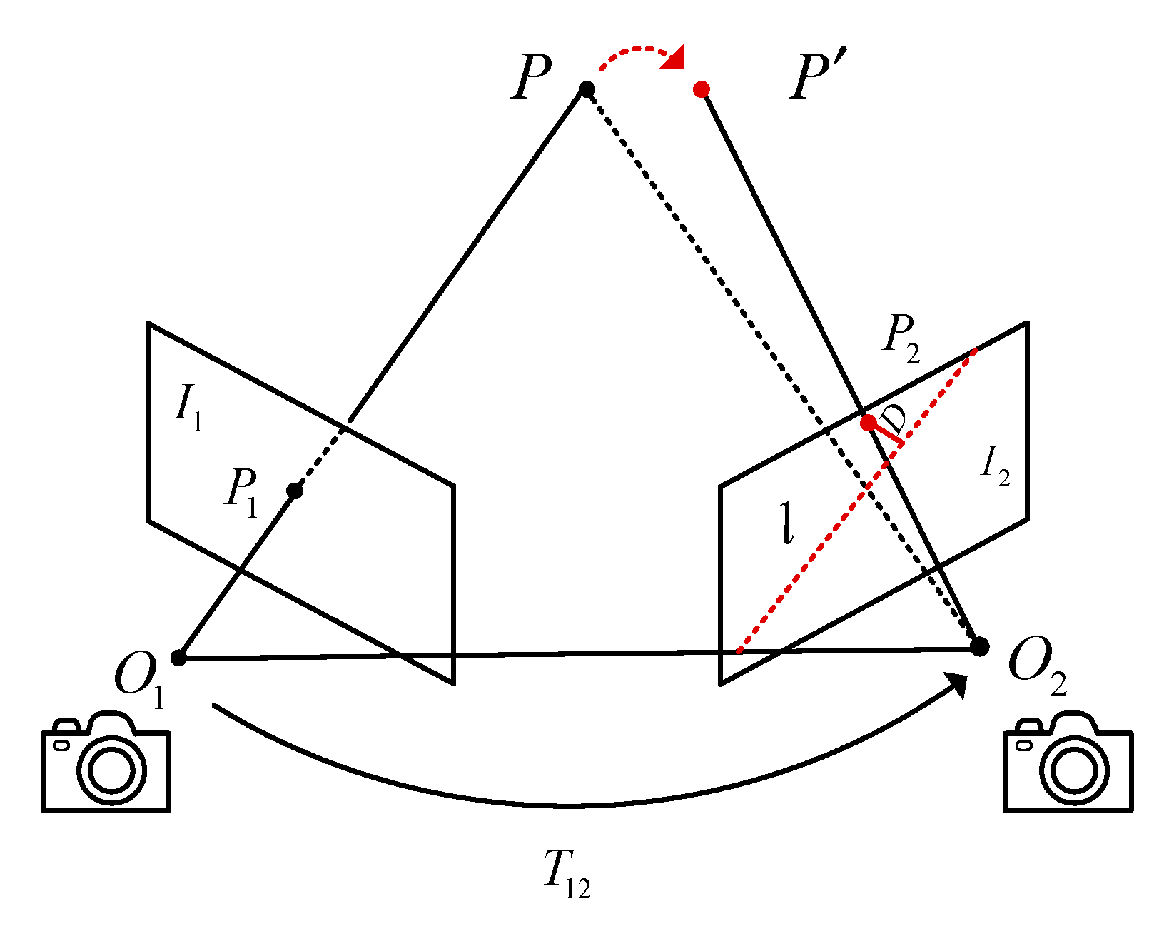
The paper combines semantic information and epipolar geometry constraints to accurately identify and remove dynamic feature points in dynamic environments. As shown in Figure 15, the epipolar geometric constraint relationship between the previous frame image and the current frame image is represented, where P is the map point and

P^{'}

represents the position of the P point in the current frame after motion.

3.3.2. Result Analysis

In order to verify the effectiveness of the YOLOD-SLAM algorithm, the paper conducted comparative experiments using two datasets: the TUM publicly available RGB-D dataset and a simulated orchard dynamic scene captured using the ZED2i binocular depth camera. The publicly available TUM RGB-D dataset includes sequences of dynamic objects with precise real-world trajectories and camera parameters. the paper uses these datasets to evaluate the algorithm proposed in the paper, compares it with the ORB-SLAM2 algorithm, and finally tests it in a dynamic shooting environment.

Relative Trajectory Error (RPE, Relative Pose Error)， By calculating the difference between the true pose and the estimated pose within the same time range, and then processing the difference, the relative trajectory error is obtained. the paper uses RPE to estimate the drift of the system very well. The calculation formula is shown below, where Ei represents the RPE value of the i-th frame.

E_{i} = {(Q_{i}^{- 1} Q_{i + Δ})}^{- 1} (P_{i}^{- 1} P_{i + Δ})

(10)

RMSE (E_{1 : n}, Δ) = {(\frac{1}{m} \sum_{i = 1}^{m} trans {(E_{i})}^{2})}^{\frac{1}{2}}

(11)

Absolute Trajectory Error (ATE) is calculated by directly subtracting the true pose from the estimated pose, which can directly reflect the accuracy and global consistency of the visual SLAM algorithm. Align the estimated value with the true value based on the timestamp of the trajectory, and then calculate the difference between the true pose and the estimated pose. The calculation formula is shown below, where trans represents translation error and rotate represents angle error.

F_{i} = Q_{i}^{- 1} S P_{i}

(12)

RMSE (F_{1 : n}, Δ) = {(\frac{1}{m} \sum_{i = 1}^{m} trans {(F_{i})}^{2})}^{\frac{1}{2}}

(13)

RMSE (F_{1 : n}, Δ) = {(\frac{1}{m} \sum_{i = 1}^{m} r o t a t e {(F_{i})}^{2})}^{\frac{1}{2}}

(14)

Where,

P_{i}, Q_{i}

refers to the true pose and estimated pose, respectively.

As shown in Table 5, the TUM RGB-D dataset is divided into multiple sequences such as sitting, walking, and table based on different usage scenarios. In the experiment of the paper, the main purpose of using the walking sequence is to include two pedestrians walking in an office scene. This sequence represents a high dynamic environment, and the sitting sequence is also used as a supplement, including two people sitting on chairs and occasionally moving. This sequence represents a low dynamic scene.

Comparing the feature extraction maps of ORB-SLAM2 and YOLOD-SLAM algorithms on the TUM dynamic sequence dataset, ORB-SLAM2 contains a large number of dynamic points in dynamic scenes, which leads to tracking loss or failure of the algorithm in dynamic environments. YOLOD-SLAM2 algorithm removes dynamic points while retaining static points within the box, improving the robustness and accuracy of the algorithm.

Calculate the error between the estimated sequence and the true value to evaluate the performance of the algorithm. Absolute trajectory error (ATE) and relative trajectory error (RPE) are often used as evaluation metrics in SLAM. ATE is very suitable for measuring global consistency of trajectories, while RPE is very suitable for measuring translational and rotational drift. The evaluation results are shown in Table 6, Table 7 and Table 8.

Based on the data in the above table, Table 6 presents the results of ATE error. YOLOD-SLAM2 has higher accuracy in fr3-walking_rpy, fr3-walking_xyz, and fr3_stingting_malf, while the error is lower compared to ORB-SLAM2 in fr3/s/xyz. Table 7 and Table 8 present the results of translational RPE error and rotational RPE error, respectively. The experimental results indicate that the table shows that YOLOD-SLAM2 has an average RMSE improvement of 97.06%, 97.23%, and 96.41% compared to ORB-SLAM2 in the high dynamic sequence fr3-walking_xyz, ATE, translational RPE, and rotational RPE, respectively. The average improvement values on the high dynamic sequence fr3-walking_rpy are 95%, 71%, 95.83%, and 95.19%, respectively. The results indicate that the dynamic feature removal method integrated in the front-end of this paper greatly improves the performance of visual SLAM in dynamic scenes. In low dynamic sequences, YOLOD-SLAM2 only has one RMSE indicator with RPE translational drift that is inferior to ORB-SLAM2, while the other indicators show slight improvement. In low dynamic environments, ORB-SLAM2 can also remove obvious dynamic features as outliers. The system has no negative impact in both low dynamic and static environments, verifying the accuracy and robustness of the YOLOD-SLAM2 algorithm.

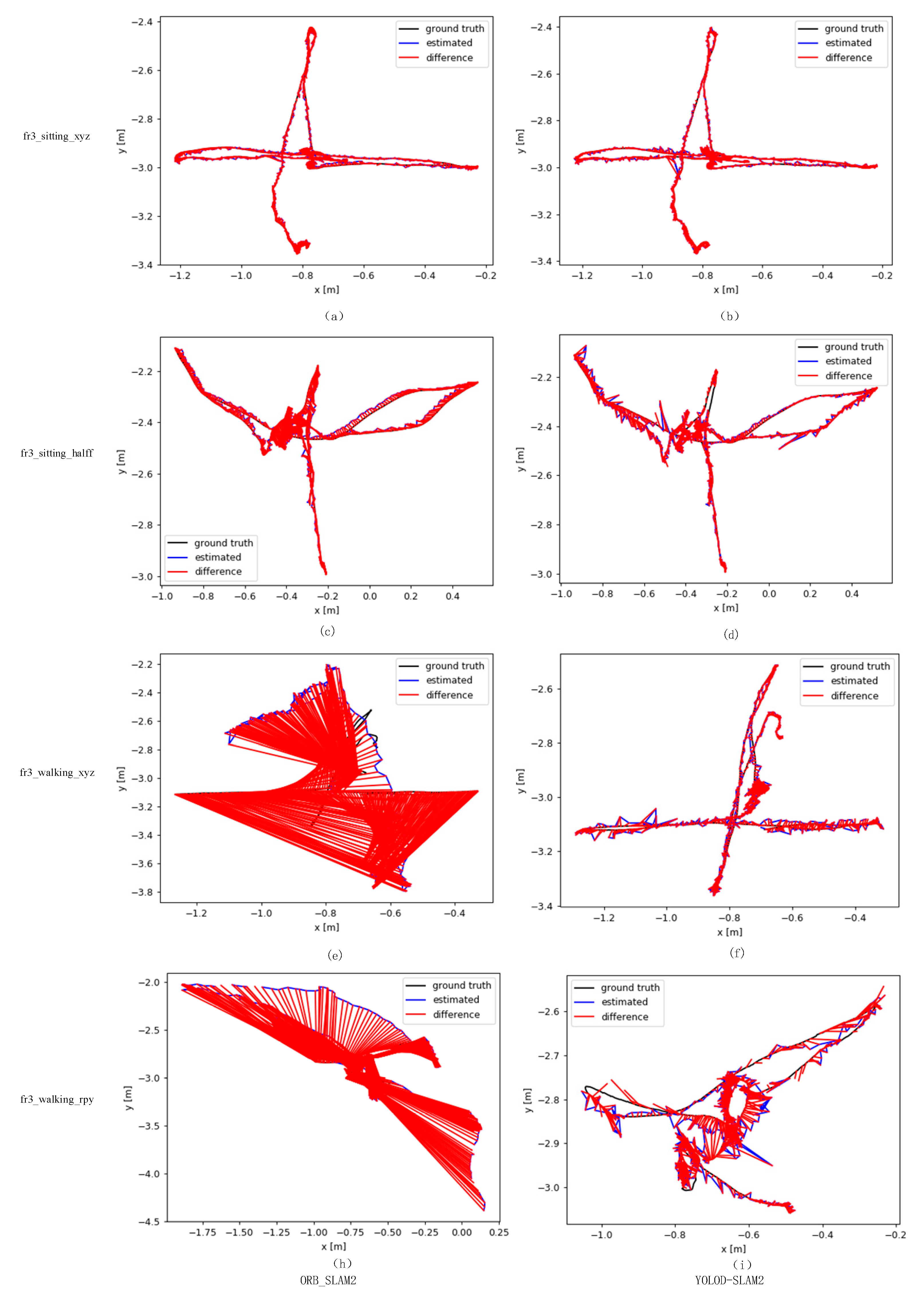
To further validate the feasibility of the algorithms, the trajectories of ORB-SLAM2 and YOLOD-SLAM2 algorithms were visualized, and the error lines between the estimated trajectories and the actual trajectories were calculated for both algorithms. As shown in Figure 17, the real trajectory is represented by a black line, the estimated trajectory is represented by a blue line, and the red line represents the difference between the real trajectory and the estimated trajectory. Each column displays, from top to bottom, the comparison between the trajectories generated by the low dynamic sequences fr3_stingting_xyz and fr3_stingting_malf, and the high dynamic sequences fr3-walking_xyz and fr3-walking_rpy, and the actual trajectories. The two graphs in each row represent the comparison of estimated trajectories for ORB-SLAM2 and YOLOD-SLAM2, respectively. The larger the red area, the greater the error.

From Figure 17, it can be seen that the trajectory diagrams of the two algorithms are similar in the first row of low dynamic sequences. In the last two high dynamic sequences, the performance of ORB-SLAM2 is significantly inferior to YOLOD-SLAM2. It can be observed that there are tracking failures in ORB-SLAM2 in the trajectories of the fr3-walking_rpy and fr3-walking_xyz sequences. In Figures 17e,h, only the true trajectory lines are present, without estimated trajectory lines.

Real time performance is a very important indicator. Table 9 shows the running time of YOLOD-SLAM2 and ORB-SLAM2 tracking processes. YOLOD-SLAM2 processes each frame of image in an average time of about 50 ms, which basically meets the requirements of real-time operation.

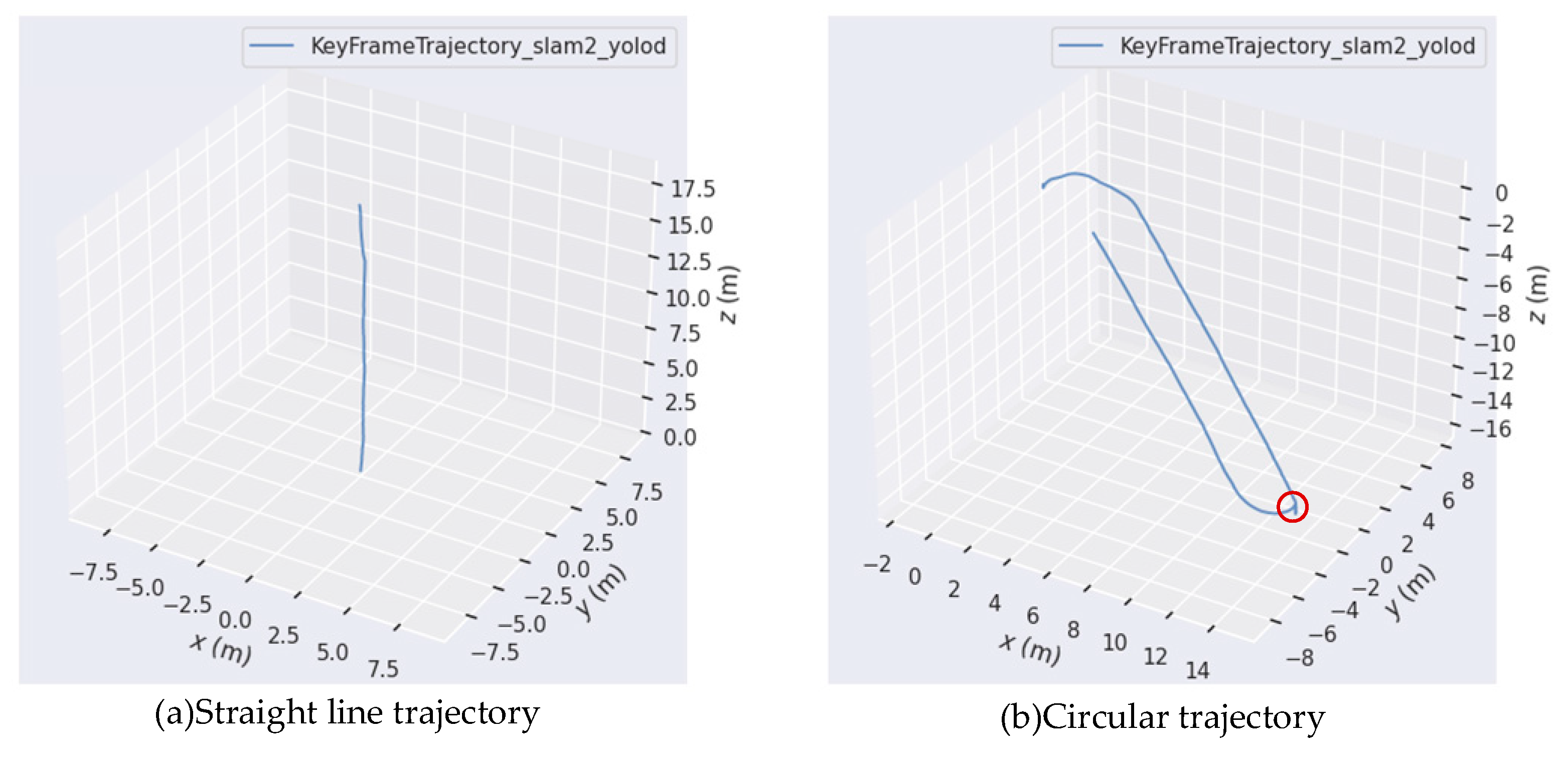
Figure 18 shows the trajectory estimation results of the algorithm proposed in this paper for a mobile car traveling along straight and circular paths in actual dynamic environments. It can be seen that in actual dynamic environments, YOLOD-SLAM2 can effectively perform pose estimation. Figure 18 (a) shows the trajectory of the car when traveling in a straight line, and Figure 18 (b) shows the trajectory of the car traveling in a circular path around a tree. The trajectory estimated by the algorithm is basically consistent with the predetermined trajectory shape. These results fully validate the effectiveness of the algorithm proposed in this paper in practical scenarios.

4. Conclusions

The paper investigates the application experiment of dynamic visual SLAM localization algorithm based on YOLOD-SLAM2 in orchard environment. The method of extracting navigation lines based on object detection proposed in the paper was tested in two scenarios of actual orchards. The average angle deviation between the navigation lines and manually labeled navigation lines did not exceed 5 °, and the average detection time was about 50ms, which meets the extraction requirements of inter row navigation lines in orchards. The distance measurement algorithm based on four zone depth comparison proposed in the paper has a relative error of less than 1% for distances within 6 meters and an average time of 34 milliseconds, which meets the needs of agricultural machinery driving between rows in orchards. The YOLOD-SLAM2 algorithm proposed in the paper achieves accurate localization. The validation results on the TUM dynamic dataset show that the RMSE indicators of ATE, translational RPE, and rotational RPE of this algorithm have improved by more than 90% on high dynamic sequences, and slightly lower than ORB-SLAM2 on low dynamic sequences, verifying the accuracy and robustness of the algorithm. The algorithm in the paper has relatively small errors in orchard environments, with absolute trajectory errors of less than 0.03m/s in ATE indicators and an average tracking time of 47ms, verifying its accuracy and real-time performance.

Author Contributions

Conceptualization, J.L. and Z.M.;Data curation, S.Y. and Z.M.; Funding acquisition, J.L.; Investigation, S.Y. and Z.M.; Methodology,S.Y. and Z.M.; Supervision, J.Q. and J.L.; Validation, S.Y. and Z.M.; Writing – original draft, Z.M. All authors have read and agreed to the published version of the manuscript.

Funding

This research was funded by Xinjiang Production and Construction Corps Key Laboratory of Modern Agricultural Machinery ,grant number XDNJ2023006.

Institutional Review Board Statement

Not applicable.

Data Availability Statement

The data presented in this study are available on request from the authors.

Conflicts of Interest

The authors declare that they have no known competing financial interests or personal relationships that could have appeared to influence the work reported in this paper.

References

Cui, B.B.; Zhang, J.; Wei, X.; Cui, X.; Sun, Z., Zhao, Y.; & Liu, Y. Improved Information Fusion for Agricultural Machinery Navigation Based on Context-Constrained Kalman Filter and Dual-Antenna RTK. Actuators. 2024,13(5):160. [CrossRef]
Sun, Y.; Cui, B.B.; Ji, F.; Wei, X.; Zhu, Y. The full-field path tracking of agricultural machinery based on PSO-enhanced fuzzy stanley model. Applied Sciences. 2022,12(15), 7683. [CrossRef]
Ji, X.; Wei, X.; Wang, A. A novel composite adaptive terminal sliding mode controller for farm vehicles lateral path tracking control. Nonlinear Dynamics. 2022, 110(3): 2415-2428. [CrossRef]
Huang, W.; Ji, X.; Wang, A. Straight-line path tracking control of agricultural tractor-trailer based on fuzzy sliding mode control. Applied Sciences. 2023, 13(2): 872. [CrossRef]
Guan, X.P. Multi-Feature Fusion Recognition and Localization Method for Unmanned Harvesting of Aquatic Vegetables. Agriculture. 2024, 14(7): 971. [CrossRef]
Zhang, L.Y. Estimating Winter Wheat Plant Nitrogen Content by Combining Spectral and Texture Features Based on a Low-Cost UAV RGB System throughout the Growing Season. Agriculture. 2024, 14(3): 456. [CrossRef]
Liu, Y.Y; Qiu, G.J; Wang N. A Novel Method for Peanut Seed Plumpness Detection in Soft X-ray Images Based on Level Set and Multi-Threshold OTSU Segmentation. Agriculture. 2024, 14(5): 765. [CrossRef]
Radcliffe, J.; Cox, J.; Bulanon, D.M. Machine Vision for Orchard Navigation. Computers in Industry. 2018, 98: 165-171. [CrossRef]
Opiyo, S.; Okinda, C.; Zhou, J. Medial axis-based machine-vision system for orchard robot navigation. Computers and Electronics in Agriculture. 2021, 185: 106153. [CrossRef]
Bochkovskiy, A.; Wang, C.Y.; Liao, H.Y.M. Yolov4: Optimal Speed and Accuracy of Object Detection. Arxiv Preprint Arxiv. 2004, 10934, 2020.
Feng, G., Wang, C., Wang, A., Gao, Y., Zhou, Y., Huang, S., Luo, B. (2024). Segmentation of Wheat Lodging Areas from UAV Imagery Using an Ultra-Lightweight Network. Agriculture, 14(2), 244. [CrossRef]
Duan, K.; Xie, L.; Qi, H. Location-Sensitive Visual Recognition with Cross-IOU Loss. arXiv preprint arXiv:2104.04899, 2021.
Abdullah, A., Amran, G. A., Tahmid, S. M., Alabrah, A., AL-Bakhrani, A. A., Ali, A. A Deep-Learning-Based Model for the Detection of Diseased Tomato Leaves. Agronomy. 2024, 14(7), 1593. [CrossRef]
Hsu, W.Y.; Lin, W.Y. Adaptive Fusion of Multi-Scale YOLO for Pedestrian Detection. IEEE Access. 2021, 9: 110063-110073. [CrossRef]
Wan, J.L.; Li, J.L. Dense Pedestrian Detection Based on Improved YOLO-v5. Third International Conference on Artificial Intelligence and Electromechanical Automation. 2022, 12329: 409-415.
Panigrahi, S.; Raju, U.S.N. DSM-IDM-YOLO: Depth-wise Separable Module and Inception Depth-wise Module Based YOLO for Pedestrian Detection. International Journal on Artificial Intelligence Tools. 2023, 32(04): 2350011. [CrossRef]
Wang, R.; Wan, W.; Wang, Y. A New RGB-D SLAM Method with Moving Object Detection for Dynamic Indoor Scenes. Remote Sensing. 2019, 11(10): 1143. [CrossRef]
Cheng, J.; Wang, C.; Meng, M.Q.H. Robust Visual Localization in Dynamic Environments Based on Sparse Motion Removal. IEEE Transactions on Automation Science and Engineering. 2019, 17(2): 658-669. [CrossRef]
Sun, Y.; Liu, M.; Meng, M.Q.H. Motion removal for reliable RGB-D SLAM in dynamic environments. Robotics and Autonomous Systems. 2018, 108: 115-128. [CrossRef]
Liu, G.; Zeng, W.; Feng, B. DMS-SLAM: A General Visual SLAM System for Dynamic Scenes with Multiple Sensors. Sensors. 2019, 19(17): 3714. [CrossRef]
Li, G.; Liao, X.; Huang, H. Robust Stereo Visual SLAM for Dynamic Environments with Moving Object. IEEE Access. 2021, 9: 32310-32320. [CrossRef]
Yu, C.; Liu, Z.; Liu, X.J. DS-SLAM: A semantic visual SLAM towards dynamic environments. IEEE/RSJ International Conference on Intelligent Robots and Systems. 2018: 1168-1174.
Badrinarayanan, V.; Kendall, A.; Cipolla, R. SegNet: A Deep Convolutional Encoder-Decoder Architecture for Image Segmentation. IEEE transactions on pattern analysis and machine intelligence. 2017, 39(12): 2481-2495. [CrossRef]
Bescos, B.; Fácil, J.M.; Civera, J. DynaSLAM: Tracking, Mapping, and Inpainting in Dynamic Scenes. IEEE Robotics and Automation Letters. 2018, 3(4): 4076-4083. [CrossRef]
He, K.; Gkioxari, G.; Dollár, P. Mask R-CNN. IEEE International Conference on Computer Vision. 2017: 2961-2969.

Figure 1. Pinhole Camera Model.

Figure 2. Pixel Coordinate sSystem.

Figure 3. YOLOv5s algorithm network structure.

Figure 4. Overall principle block diagram of ORB-SLAM2.

Figure 6. Problem diagram of extracting navigation lines in Scenario 1.

Figure 7. Problem diagram of extracting navigation lines in scenario 2.

Figure 8. Navigation line extraction diagram.

Figure 9. Navigation line extraction in different orchard scenes.

Figure 10. Schematic diagram of evaluation indicators.

Figure 11. Angle deviation.

Figure 12. Schematic diagram of algorithm flow.

Figure 13. Pedestrian Distance Measurement Experiment.

Figure 14. Left image and depth map of binocular camera.

Figure 15. Geometric Constraints of Polar Lines.

Figure 17. Comparison of Algorithm Trajectory.

Figure 18. Actual Orchard Environment Trajectory Map.

Table 1. Analysis of Navigation Line Extraction Error Index in Different Scenarios.

Scenario	Number of images	Average angle deviation/(°)	Standard deviation of angle deviation/(°)
Scenario 1	100	1.4797	1.3675
Scenario 2	100	2.8942	2.7102

Table 2. Comparison of Algorithms in Different Scenarios.

Scenario	Number of images	Accurate extraction frame rate	Extraction accuracy	Average extraction time/ms
Scenario 1	100	97	97%	47.98
Scenario 2	100	94	94%	56.11

Table 5. Description of TUM RGB-D Dataset.

	Sequence	Duration/s	Length/m	Content
Scenario of people sitting on a chair	fr3_sitting_xyz	42.50	5.496	Maintain the same angle and move the camera along three directions (x, y, z)
Scenario of people sitting on a chair	fr3_sitting_half	37.15	6.503	The camera moves on a small hemisphere with a diameter of 1m
Scenario of people walking around	fr3_walking_xyz	28.83	5.791	Maintain the same angle and move the camera along three directions (x, y, z)
Scenario of people walking around	fr3_walking_rpy	30.61	2.698	The camera rotates along the main axis (row, pitch, yaw) at the same position.

Table 6. ATE Error (m/s).

Sequence	ORB-SLAM2		YOLOD-SLAM2		Improvements
Sequence	RMSE	S.D.	RMSE	S.D.	RMSE	S.D.
fr3_sitting_xyz	0.0111	0.0052	0.0108	0.0056	2.91%	-7.56%
fr3_sitting_half	0.0287	0.0132	0.0204	0.0124	29.03%	6.27%
fr3_walking_xyz	0.6102	0.1677	0.018	0.0094	97.06%	94.39%
fr3_walking_rpy	0.6994	0.3372	0.03	0.0177	95.71%	94.76%

Table 7. Translation T RPE Error (m/s).

Sequence	ORB-SLAM2		YOLOD-SLAM2		Improvements
Sequence	RMSE	S.D.	RMSE	S.D.	RMSE	S.D.
fr3_sitting_xyz	0.0117	0.0057	0.0157	0.0076	-33.79%	-33.5%
fr3_sitting_half	0.0413	0.0199	0.0293	0.0163	29.00%	18.02%
fr3_walking_xyz	0.922	0.5034	0.0256	0.0125	97.23%	97.51%
fr3_walking_rpy	1.0223	0.5483	0.0427	0.0229	95.83%	95.82%

Table 8. Rotation R RPE Error (°/s).

Sequence	ORB-SLAM2		YOLOD-SLAM2		Improvements
Sequence	RMSE	S.D.	RMSE	S.D.	RMSE	S.D.
fr3_sitting_xyz	0.4798	0.2461	0.5863	0.3007	-22.19%	-22.19%
fr3_sitting_half	0.8586	0.356	0.7806	0.3743	9.09%	-5.13%
fr3_walking_xyz	18.787	10.161	0.6746	0.4035	96.41%	96.03%
fr3_walking_rpy	19.98	11.62	0.9617	0.523	95.19%	95.50%

Table 9. Average Time/ms.

Sequence	ORB-SLAM2	YOLOD-SLAM2
fr3_sitting_xyz	17.99	42.74
fr3_sitting_half	20.89	48.03
fr3_walking_xyz	20.73	42.69
fr3_walking_rpy	21.65	41.73

Disclaimer/Publisher’s Note: The statements, opinions and data contained in all publications are solely those of the individual author(s) and contributor(s) and not of MDPI and/or the editor(s). MDPI and/or the editor(s) disclaim responsibility for any injury to people or property resulting from any ideas, methods, instructions or products referred to in the content.

© 2024 by the authors. Licensee MDPI, Basel, Switzerland. This article is an open access article distributed under the terms and conditions of the Creative Commons Attribution (CC BY) license (http://creativecommons.org/licenses/by/4.0/).

Copyright: This open access article is published under a Creative Commons CC BY 4.0 license, which permit the free download, distribution, and reuse, provided that the author and preprint are cited in any reuse.

MDPI Initiatives

Important Links

Choose an area of interest and we will send you notifications of new preprints at your preferred frequency.

Disclaimer