Preprint
Article

A Novel Modeling Optimization Approach for a Seven-channel Titania Ceramic Membrane in an Oily Wastewater Filtration System Based on Experimentation, Full Factorial Design, and Machine Learning

Altmetrics

Downloads

68

Views

63

Comments

0

A peer-reviewed article of this preprint also exists.

This version is not peer-reviewed

Submitted:

12 August 2024

Posted:

12 August 2024

You are already at the latest version

Alerts
Abstract
This comprehensive study looks at how operational conditions affect the performance of a novel seven-channel titania ceramic ultrafiltration membrane for the treatment of produced water. A Full factorial design experiment (23) was conducted to study the effect of the cross-flow operating factors on the membrane permeate flux decline and the overall permeate volume. Eleven experimental runs were performed for three important process operating variables: Transmembrane Pressure (TMP), Crossflow Velocity (CFV), and Filtration Time (FT). Steady final membrane fluxes and permeate volumes were recorded for each experimental run. Under the optimized conditions (1.5 bar, 1 m/s, and 2 hours), the membrane performance index demonstrated an oil rejection rate of 99%, a flux of 297 liters/m2·hr (LMH), a 38% overall initial flux decline, and a total permeate volume of 8.14 L. The regression models used for the steady-state membrane permeate flux decline and overall permeate volume led to the highest goodness of fit to the experimental data with a correlation coefficient of 0.999. A Multiple Linear Regression method and an Artificial Neural Network approach were also employed to model the experimental membrane permeate flux decline and analyze the impact of the operating conditions on membrane performance. The predictions of the Gaussian regression and the Levenberg-Marquardt backpropagation method were validated with a determination coefficient of 99 % and a mean square error of 0.07.
Keywords: 
Subject: Engineering  -   Chemical Engineering

1. Introduction

Produced water (PW) is a category of oily wastewater generated by many industrial activities, including oil and gas operations. These industries produce substantial crude oil quantities and massive volumes of wastewater. PW is a mixture of water, dissolved and undissolved oil, aromatics, hydrocarbons, gasses, organic materials, salts, heavy metals, suspended solids, bacteria, corrosion and treatment chemicals, residual production-line additives, toxic pollutants, and other chemicals [1,2,3,4]. As a response to the harmful effect of PW, new environmental regulations and wastewater treatment of PW became mandatory to meet discharge limits [5]. The search for novel inexpensive PW treatment technologies, simple to use, and easy to maintain has lately gained prominence. Membrane technology has grown in popularity as a viable filtration approach for oily wastewater treatment [6]. Membrane filtration is commonly associated with low energy consumption, cost-effectiveness, and minimal footprint characteristics [7]. Regardless of its operating potential, membrane technology’s growing adoption is hampered by membrane fouling. Fouling is the deposition of rejected oil, pollutants, colloidal particles, and bacteria over the membrane surface, causing surface deterioration, a decline in the membrane permeation rate, and a rise in filtration costs [8]. The significance of fouling in the membrane technology field is well-known and has been frequently investigated. Researchers typically built physical, empirical, or semi-empirical models to analyze the process mechanism under various conditions. However, these models often fail to explain and monitor the data variation patterns under the operating conditions for a complex system with a complex feed composition [9], ceramic membrane pores tortuosity blocking process [10], and turbulent hydrodynamic conditions. Therefore, understanding the membrane filtration system characteristics, properties, and components is insufficient for understanding membrane fouling. Various mechanistic models have been proposed from dead-end to crossflow filtration to describe the fouling phenomenon but are limited by the concentration polarization pre-fouling development [11]. As a result, it is essential to develop alternative methodologies to overcome the complexity of the filtration system, such as statistical modeling and Artificial Intelligence methods, to assist fouling system modeling by avoiding the intricate theories that underpin the process. These soft-computing methods are reliable, with problem-solving abilities, are cost-effective and result-oriented [12].
Statistical modeling approaches [13,14,15,16,17,18,19,20,21] are widely used to estimate the correlation between explanatory variables and response values in polynomial regression equations. Studying different operating conditions one by one is time-consuming and costly [22]. A statistical method such as full factorial design can circumvent this by looking at all the parameters and their impact for each level of operating condition [23,24]. Outcomes at all combinations of factor levels are measured. Variation of factor levels is performed, instead of one at a time, to explore all interactions and their effect on target responses. In this study, each experimental run factor was performed at two levels. All sequences of the factor levels are integrated into the experimental runs. The 2-level factorial design thoroughly investigates the factors domain, giving important information for a few runs per factor [25].
Artificial intelligence (AI) techniques, such as Multiple Linear Regression (MLR) and Artificial Neural Networks (ANNs), can be a viable choice for predicting the process design response based on the operating input parameters [26,27,28,29,30,31,32,33,34,35,36,37,38]. The MLR can map a nonlinear process and estimate the response values for multiple regressors using a polynomial equation [39,40]. ANN has shown to be an eminent technique because it iterates, learns, and stores data to forecast the system’s response effectively. A fundamental advantage of AI modeling is its independence of the filtration process and capability to predict the system output without any prior knowledge or information about the feed characteristics or the membrane surface properties [40]. ANN models are mainly trained using the operating conditions and collected experimental data. Due to ANN’s flexible application, and fitness to learn from the data, it gained much acceptance in the wastewater management field. The ANN can be trained with the Levenberg–Marquardt (LM) Backpropagation algorithm (trainlm) [39]. A two-layer feed-forward network with hidden sigmoid neurons and one linear output neuron (fitnet) trains the network to fit the inputs and targeted response. Given reliable data and enough neurons in its hidden layer, the training algorithm can arbitrarily fit multi-dimensional variants mapping problems [41]. Moreover, it automatically stops when generalization stops improving. ML-ANN backpropagation successfully delivers a practical regression approach and analysis of the operating conditions’ variations for predicting the permeate flux in oily wastewater systems compared to other standard modeling techniques.
In this study, the assessment of the full factorial design, multiple linear regression analysis, and neural network techniques for the predictions and optimization of the operating conditions (TMP, CFV, and FT) of an ultrafiltration (UF) titania ceramic membrane was performed, treating a synthesized produced water feed representing the PW of the Bakken reservoir in Western Canada. An analysis of variance was performed to identify the significant impact of the univariate and multivariate operating conditions on the membrane permeate flux and yield permeate volume. The response values and their sensitivity variation to the operating conditions were plotted in contours to depict the optimized process operating regions. The composite desirability function was used as an optimization method to assess the operating variables settings and maximize the permeate flux and volume [4]. Furthermore, the membrane rejection capacity for each experimental run was analyzed and reported under various operating settings. Finally, MRL and ANN-trained models were used to fit the membrane permeate flux decline data and provide an algorithm for forecasting the system behavior under various operating parameters. The models’ statistical goodness-of-fit was validated by employing the correlation coefficient and mean squared roots as the statistical keys of performance metrics.
Table 1 is an overview of published filtration studies for oily wastewater found in the literature with details of the operating variables studied, optimization method used, and resulting performance.

2. Theory

For the analysis of the experimental data, a full factorial design [42,43,44,45], multilayer regression model algorithms (MLR), and artificial neural network (ANN) [46,47,48] were selected to predict the membrane permeate flux. Recently, researchers have extensively applied Artificial Intelligence to optimize the process operating conditions targeting cost-effectiveness and time-saving experimental design [49,50,51,52,53,54].

2.1. Full Factorial Design Methodology

In this study, a 23 full factorial design was employed to screen the impact of the transmembrane pressure, crossflow, and filtration time, as the primary independent factors, on membrane performance. Additional factors such as pH, feed oil content, and temperature were maintained constant during this experiment [1]. The studied factors are often evaluated in the literature and considered the most critical parameters in membrane process optimization [2,13,14,15]. The levels and symbols of each independent factor were set for high (+1), middle (0), and low (−1), as reported in Table 2. The factors’ levels were combined to capture the full interactions of the operating conditions and their impact on the membrane performance. A total of 11 runs were performed to obtain a quadratic regression model of 8 runs and 3 center points (equation (1)). The experiments were performed randomly to minimize experimental errors [55]. The factor ranges were identified based on a review of the literature [2,4,14,15,55], the setup capabilities, and considering experimental costs. Table 2 illustrates the coded levels of each independent factor for the full factorial design experiment.
A robust data analysis, statistical, and process improvement software tool, Minitab 19, was used to predict, visualize, and analyze the experimental data. A quadratic regression model was developed to predict the response values [4]:
Y k   = b 0 + i = 1 n b i   x i   + i < j n b i j   x i   x j   + i = 1 n b i i   x i 2 + S e  
where Yk (k = 1,2) is the predicted response used as a dependent variable; to predict Y1: the permeate flux and Y2: permeate volume, respectively. xi (i= 1, 2, and 3) designates the selected factors, x1: TMP, x2: CFV, and x3: FT, respectively. In this equation, b0 is a model constant coefficient, and Se is the statistical error (residual), bi (i=1, 2, 3), bij (i = 1, 2, 3; j = 1, 2,3; i < j), and bii, denote the linear, interactional, and quadratic regression model coefficients, respectively. These coefficients are approximated by multiple linear regression analysis. The goodness of fit of the full factorial polynomial model was quantified with the coefficient of determination (R2) and the lack of fit. A variance analysis was carried out to ascertain the significance of the regression factors and their interactions. A significant level P-value for the model below 0.05 was deemed meaningful and considered significant more than 95%. The measured responses for the permeate flux decline and permeate volume were denoted Jni (final steady permeate flux measured in LMH) and Ynf (final net permeate volume measured in litres (L)). In each experiment, the permeate flux decline, steady-state total permeate volume (Table 3), rejection capacity, and permeate turbidity (Table 4) were used to quantify the membrane performance and fouling control.

2.2. Multiple Linear Regression Method

The multiple linear regression (MLR) model is commonly employed as an empirical model to estimate and explore the functional link between the dependent responses’ target values and the independent explanatory regressor variables. MLR is employed when more than one predicted response variable is involved. MLR analysis prompts estimating the regression coefficients of the fitted linear model equation by the ordinary least squares method to predict the experimental data. Multiple linear regression model (equation (2)), with n independent variables, xi (i = 1,…, n) and yi (i>1) dependent response is written in terms of the regression coefficients as follows [39,56]:
y i   = µ 0   + j = 1 n µ j x i j + e i ,   i = 1 , 2 , . , m  
where µ0 and µj (j= 1,…, n) are the regression coefficients and ei is the model regression error.
The least squares method finds the best estimation coefficient µj in equation (2) for the descriptive data set to minimize the sum of the squared errors. The least squares function is represented by equation (3) or (4):
S = i = 1 m e i 2
  S = i = 1 m y i µ 0   j = 1 n µ j x i j 2
The objective least squares function S is minimized according to the regression coefficients µ0, µ1,…, µn. The terms’ coefficients b0, b1,…, bn, fulfill the equations (5) and (6), respectively [56].
S µ 0 = 2 i = 1 m y i b 0 j = 1 n b j x i j = 0  
S µ j = 2 i = 1 m y i b 0 j = 1 n b j x i j   x i j = 0  
Data for the eleven experimental runs were used to train the regression models, including the linear regression models, Regression trees, Support vector machines, Gaussian process regression models, and Ensembles of regression trees (supplementary materials C, Figure S1). The regression models’ data input were the TMP, CFV, and FT of each experimental run, and the response was the permeate flux. Matlab R2020b was used as a technical computing tool for data analysis and visualization. Nineteen regression models were trained (Supplementary Materials C, Figure S2) by applying cross-validation folds of five to avoid the model overfitting. Then the performance was compared side-by-side using their statistical parameters R-squared, RMSE, MSE, and MAE (equations (7) - (12))
  • R-squared (the coefficient of determination) is a goodness-of-fit measure for strength linear regression association between the trained model response and experimental data. The closer to one, the better the model is.
    R 2 = 1 R S S T S S
    R S S = i = 1 n F l u x i F l u x ^ 2
    T S S = i = 1 n F l u x i F l u x ¯ 2
    where RSS = Residuals sum of squares; TSS = Total sum of squares; F l u x ¯ = mean value of the experimental data set; F l u x ^ = predicted flux value; and Fluxi = the true flux value.
  • RMSE (Root mean square error) is the root mean of residuals (model error prediction). RMSE depicts the standard deviation of the residuals around the model regression fit. The smaller the value, the better the model is (Equation (10)).
    R M S E = i = 1 n F l u x i F l u x ^ 2 n
  • MSE (Mean squared error) is the average squared residuals between the predicted and observed paired response values. MSE is the Square of the RMSE. The smaller the MSE, the better the regression model (Equation (11)).
    M S E = 1 n × i = 1 n F l u x i F l u x ^ 2
  • MAE (Mean absolute error) is an average of the positive residuals between predicted and actual responses. The smaller the MAE, the better the regression model (Equation (12)).
    M A E = 1 n × i = 1 n F l u x i F l u x ^

2.3. Artificial Intelligence Method

An important use of the ANN technique is the prediction of the process’s best operating parameters when one or more input variables vary [12,39,53,57,58]. In this study, ANN models were built by varying three input parameters: TMP, CFV, and FT [12,51,59] to predict the membrane permeate flux.
ANNs are artificial intelligence computational algorithms inspired by human biological neuron systems. ANNs are extensively used in experimental design to reduce costs and optimize conventional process performance [60]. ANNs are applied in numerous engineering fields to solve supervised and unsupervised learning problems such as classification, regression, and clustering [61,62]. It is vital to investigate the architecture of the artificial neural network to better comprehend its operation (Figure 1) [39]. ANN architecture is a neural topology connecting the input neurons and the output. These neurons are linked together and layered to construct a nonlinear operating system. The number of input data defines the number of the neurons’ input layer. The topology of the ANN network mostly depends on the number of hidden layers, neurons in each layer, and the type of transfer function processing the input data. The final output layer performs the final output computation [53]. This study selected to use of the feed-forward Levenberg-Marquardt (LM) backpropagation training algorithm [63,64,65]. This transfer function uses a Jacobian for simulations, assuming a control performance function (MSE) [66]. The algorithm looks to be the quickest way to train moderate-sized backpropagation neural networks, up to several hundred weights. It is also easy to implement in MATLAB software since the matrix equation solution is a built-in function. As a result, its characteristics become much more evident in a MATLAB setting [61].
The ANN training stops when generalization halts learning, as quantified by an increase in the mean square error and a decline in the model performance [62]. In supervised training, for a given input/output data set, the ANN algorithm can provide an optimal mapping process to predict the collected targeted experimental data based on the independent explanatory operating conditions parameters [66]. The iterative neural network learning process builds a probability-weighted relationship between the input and output data. Data is stored within the neural network throughout the training while comparing the experimental target response and model predicted value. ANN adjusts the weight coefficients to minimize the error intricated by the selected transfer function until the threshold is respected. Successive adjustments will be performed until the training algorithm fits the best target output. The Matlab ANN Toolbox was mainly employed in this study analysis. The ANN architecture used in this study is presented in Figure 1.
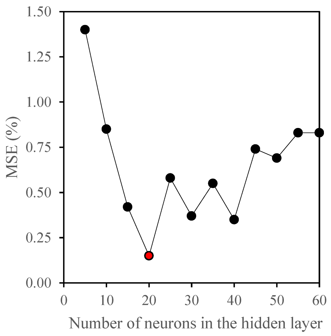
To apply ANN to the collected data, we investigated the influence of variation in the number of neurons on the training performance. A trial-and-error method was applied to determine the optimum number of neurons. Numerous models with incremental hidden layer numbers of neurons from 5 to 60 were studied, and their mean squared error (MSE) was documented and compared. Figure 2 identified the minimum MSE percentage for twenty neurons as the best ANN network configuration. Another performance parameter is the R-squared (coefficient of determination (R2)), which designates the model’s goodness of fit to predict the collected experimental data. MSE and R-squared are parameters used to select the best model that fits the experimental data set.
Consequently, an ANN model with 20 neurons was employed for further simulation and analysis. A total number of experimental data for samples between 1200 and 2400, depending on the filtration time variable (one to two hours), were considered for each model analysis. In this study, the gathered experimental data were divided into 80% for the training model, 10% for validation, and 10% for testing.
For model performance comparisons, the mean squared error percentage (MSE (%)) is computed using the following equation (13):
M S E   ( % ) = M S E M a x   ( f l u x ) × 100

3. Materials and Methods

3.1. Materials

A seven-channel ceramic membrane of 25 mm diameter was acquired from Tami Industries (Nyons, France) and cut into 305 mm pieces to match the membrane housing unit size. Bakken light oil from western Canada (Saskatchewan) was used in all experiments with a measured viscosity of 5.23 cP and a density of 0.87844 g/cc at 22.5 ℃. Reverse osmosis (RO) was utilized to prepare the ultrapure deionized water (DI, <5 ppb TOC and <0.1 colony-forming units of a microorganism/mL) using an ultraviolet (UV) water purification system (EMD Millipore, 2012, Burlington, MA, USA). The supplementary chemicals for the ultrafiltration ceramic membrane regeneration and Horiba S-316 oil/solvent extraction were purchased and used as received (Table 5).

3.2. Feed Synthesis and Characterization

The laboratory-synthesized produced water feed of ~200 ppm was prepared by mixing reverse osmosis water, Bakken light oil, and Sodium dodecyl sulfate (SDS), used for oil droplet stability, in the ratios of 2 L, 4.5 mL, and 0.3 mM, respectively. The 2 L of PW emulsion was mixed for two minutes using a commercial blender at 19,000 rpm with variable pulses to achieve a homogenous and stable feed mixture. This procedure was repeated for a total volume of 24 L (12 batches) required for each experiment. The feed water properties, such as oil content, chemical oxygen demand (COD), turbidity (TNU), pH, zeta potential, feed mean droplet size, density, and viscosity were measured and reported in Table 6. The experimental instruments employed for feed water characterization are listed in Table 7.

3.3. Ceramic Membrane Characterization

The seven channels of a UF ceramic membrane (supplementary material, Figure S1) were used to treat synthesized water feed using the LabBrain filtration unit fabricated by LiqTech International (Hobro, Denmark). Fundamental membrane characteristics and properties such as ceramic membrane morphology, pore size, molecular weight cutoff (MWCO), retention capability, permeability, ceramic membrane geometry/dimensions, and thermal/chemical resistance are reported in Table 8. The ceramic membrane surface wettability is investigated by measuring the contact angle of water and oil droplets’ adhesion to the membrane surface. Figures S2 and S3 (supplementary material) depict the membrane surface super-hydrophilicity and oleophobicity properties with a contact angle of 35 and 135°, respectively.

3.4. Crossflow Filtration System Description

In this study, a LabBrain CFU022 automated crossflow ceramic membrane filtration unit was employed to perform eleven batch-mode experiments (Figure S3). Figure S4 presents a schematic diagram of the LabBrain Proportional and Integral (P&I) control loop diagram system. The unit can operate in three modes, either manually or automatically: constant transmembrane pressure, constant feed crossflow, and constant permeate flow. To enhance the ceramic membrane’s high permeability water flow, the UF membrane was pre-experimentally prepared by a progressive submersion in deionized water and then left in a bath for an additional twelve hours to fully evacuate any trapped air from the membrane pores. The membrane element was installed and fastened to the cylindrical housing cell. A 24 L feed water emulsion was synthesized, characterized, and immediately added to the oily wastewater container to run the experiment. The speed pump level and the concentrate valve opening percentage were used to gradually adjust the settings of the filtration unit for CFV and TMP operating values. All data and operating parameters of the valves’ actual openings, transmitters, transmembrane pressure, and flux were automatically logged into the unit’s internal memory every 3 seconds. The concentrate was directed to the feed tank for continuous filtration. Once measured, the permeation flow is returned to the oily water container to keep a constant feed concentration. The membrane oil rejection performance was calculated using the following equation (14):
R e j e c t i o n   % = 1 C p C f   x   100
where Cf and CP are the oil content of the feed and permeate, respectively, in ppm.
Following each experiment, the filtration system was carefully rinsed and drained using reverse osmosis water (50 ℃), Sodium hydroxide (50 ℃), and Phosphoric acid (85 ℃), respectively, to eliminate oil, pollutants, and impurities until reaching the ceramic membrane initial flux recovery of 99% (Appendix A).

4. Results and Discussion

Membrane filtration in crossflow mode was often investigated by researchers as a prominent technique for fouling control and mitigation [67]. This study is a comprehensive investigation of the impact of operating conditions on the membrane performance. The optimal conditions were examined using full factorial design, multiple linear regression analysis, and artificial neural networks. A regression model is presented for the permeate flux and volume for the full factorial design. The MLR was employed for learning regression analysis; several algorithms were tested to select the best-fitting model and predict the permeate flux. Finally, the Artificial Neural Network-based approach was applied to fit the membrane flux decline data.

4.1. Full Factorial Design Analysis

4.1.1. Membrane Performance

This study investigated three operating parameters to examine their influence on two response parameters i.e. the membrane flux and the steady-state permeate volume. Eleven experimental runs were performed, and the membrane rejection and permeate turbidity were recorded. The titania ceramic membrane demonstrates an excellent rejection capability between 91% and 99% for the different operating sets of conditions (Table 7 and Table 8). This performance is similar to the reported research outcome in [68,69] for similar ceramic membranes.
Each experiment rejection test was performed to evaluate oil rejections, amongst others (Table 8). Experimental runs 5 (+1, +1, +1) and 6 (+1, +1, -1) demonstrate the best oil rejections attaining 97% and 98% for an overall permeate oil content <= 3 ppm, respectively. Similarly, these runs also match those with the highest permeate flux and permeate volume of 297 and 341 LMH and 8.14 and 7.82 L, respectively.
For an initial oil feed of ~200 ppm, the permeate oil content was below ~5 ppm for all the experimental runs. A configuration of a TMP of 1.5 bar (level +1) and a CFV of 1m/s (level +1) for a filtration time of either one or two hours (level -1 or +1) led to the best performance for the titania membrane. The optimized design was achieved for (+1, +1, +1) with an overall membrane performance, flux, and permeate volume of 297 LMH and 8.14 L, respectively. Measurements were performed twice, and the averages with the standard deviations were reported.

4.1.2. Statistical Analysis

To understand the effect of the operating conditions (TMP, CFV, and FT) and their interactions on the membrane performance and fouling mitigation. An Analysis of Variance (ANOVA) was performed to illustrate the results of the full factorial design experiment. Table 9 and Table 10 summarize the analysis of variance for the membrane flux and permeate volume, respectively. The results of P-values for each model depicted that the values are closer to zero, reflecting a higher significance of the regression models for both responses. For a CI of 95%, a P-value below 0.05 means statistically that the explanatory factor or their interaction is significant. The F-value demonstrates the degree of the impact of these factors on the membrane’s overall performance. For a CI of 95%, the empirical regression models for the two responses are presented by the following polynomial equations (15) and (16):
F l u x   ( L M H ) = 210.75 + 56.75   T M P + 35.75   C F V 11.5   F T + 15.75   T M P × C F V 2.00   T M P × F T 3.00   C F V × F T 5.50   T M P × C F V × F T
P e r m e a t e   ( L ) = 7.031 + 0.606   T M P + 0.184   C F V + 0.149   F T + 0.159   T M P × C F V 0.026   T M P × F T 0.019   C F V × F T + 0.056   T M P × C F V × F T
The coefficients of determination (R2) of the two models, flux and permeate volume, were 99.99% and 99.98%, respectively. The adjusted terms (R-sq(adj)) were 99.95% and 99.88%, respectively, indicating that the two proposed models predicted well more than 99% of the experimentally collected data [70].
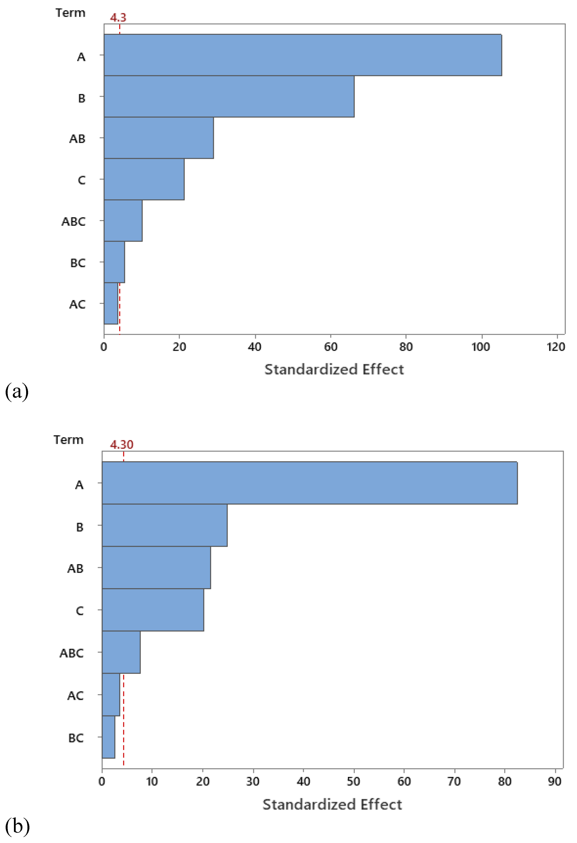
Figure 3 presents the Pareto chart to demonstrate the absolute values of the standardized effects of the terms T-values in descending magnitude effect. The reference line indicates the factors’ significant statistical effects on the responses’ values. The critical T-values for the membrane flux and permeate volume were both 4.30 at a CI of 95%. In the Pareto chart, the explanatory factors and their interactions that cross the reference line are statistically significant. The regressor parameters’ effect and their interactions are readily exhibited in Figure 3 where A>B>AB>C>ABC>BC for flux and A>B>AB>C>ABC for the permeate volume.
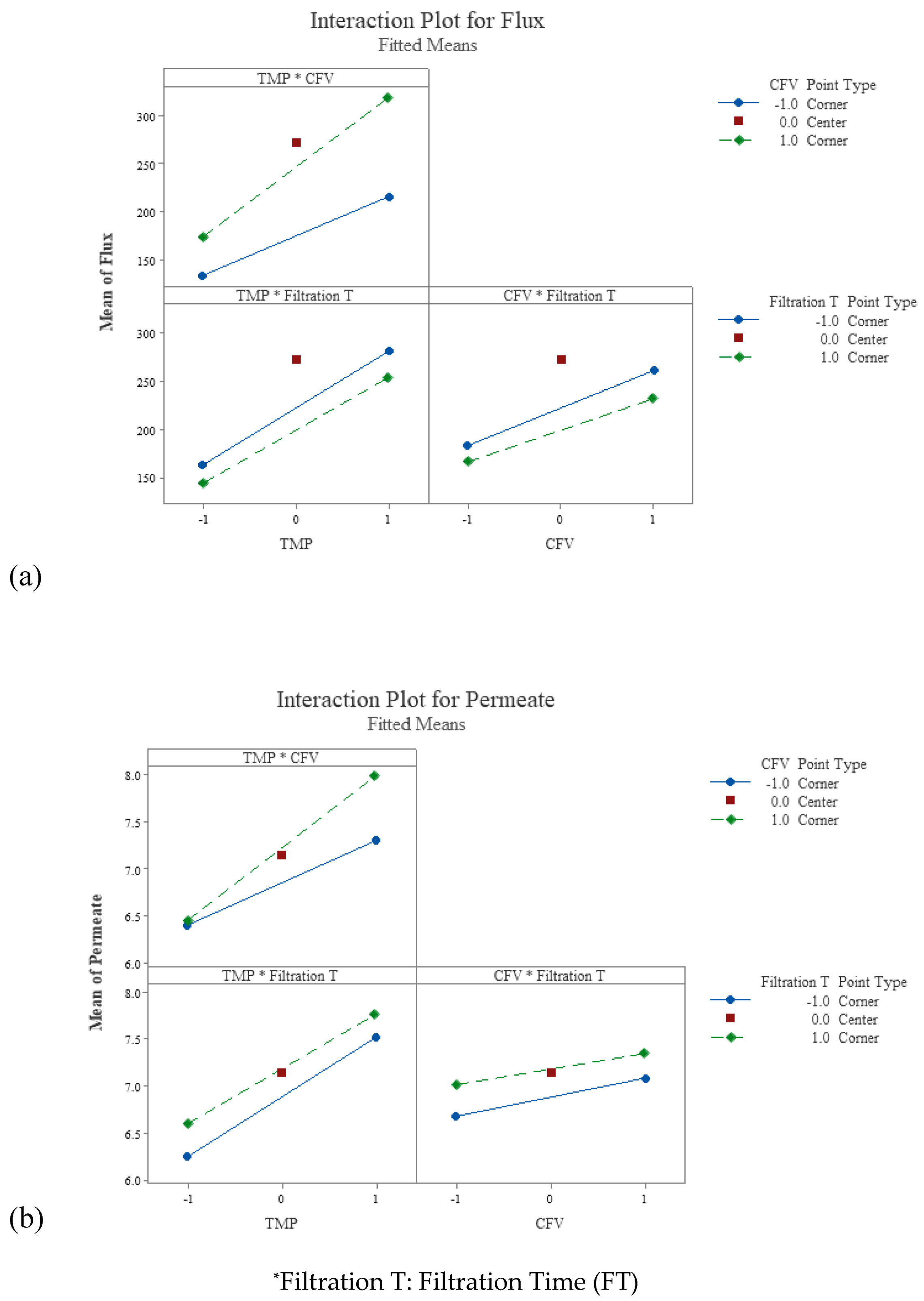
The factorial plots for flux and permeate volume (Figure 4) provided a complete visualization of the two-way interaction effects between the independent predictor’s factors and the mean response values. In each interaction block, the main effect of the regressors exists when the lines (solid and dashed) are not horizontal, indicating that the mean response values vary with the predictors’ interactions. The steeper the lines’ slope, the higher the main effect magnitude and the interaction between the explanatory variables.
Figure 4(a) top-left shows that the relationship between the membrane flux and TMP depends on the CFV variation. For CFV at the higher level +1 (the dashed green line), the mean flux varies from 174 to 319 LMH (145 LMH increase). In contrast, at lower level -1 (the solid blue line), the membrane flux varies from 134 to 216 LMH (82 LMH increase) with the variation of TMP from -1 to +1 level.
For the TMP at the lower level, -1, the variation of the CFV from the lower level -1 to the higher level +1 increases the mean flux from 134 to 174 LMH (40 LMH variation). Whereas, at the TMP with a higher level of +1, the variation of CFV from a lower to a higher level increased the mean flux from 216 to 319 LM (103 LMH variation). This indicated that the interaction between the CFV and TMP tremendously affects the membrane flux. Similarly, in Figure 4(b) top left, the interactions of the TMP × CFV were significant. However, the interaction of TMP × FT and CFV × FT was insignificant (Figure 3(b)). Thus, the three-way interactions TMP × CFV × FT were crucial and significant at CI 95% for both responses membrane flux and permeate volume (Table 9 and Table 10 and Figure 3 and Figure 4).
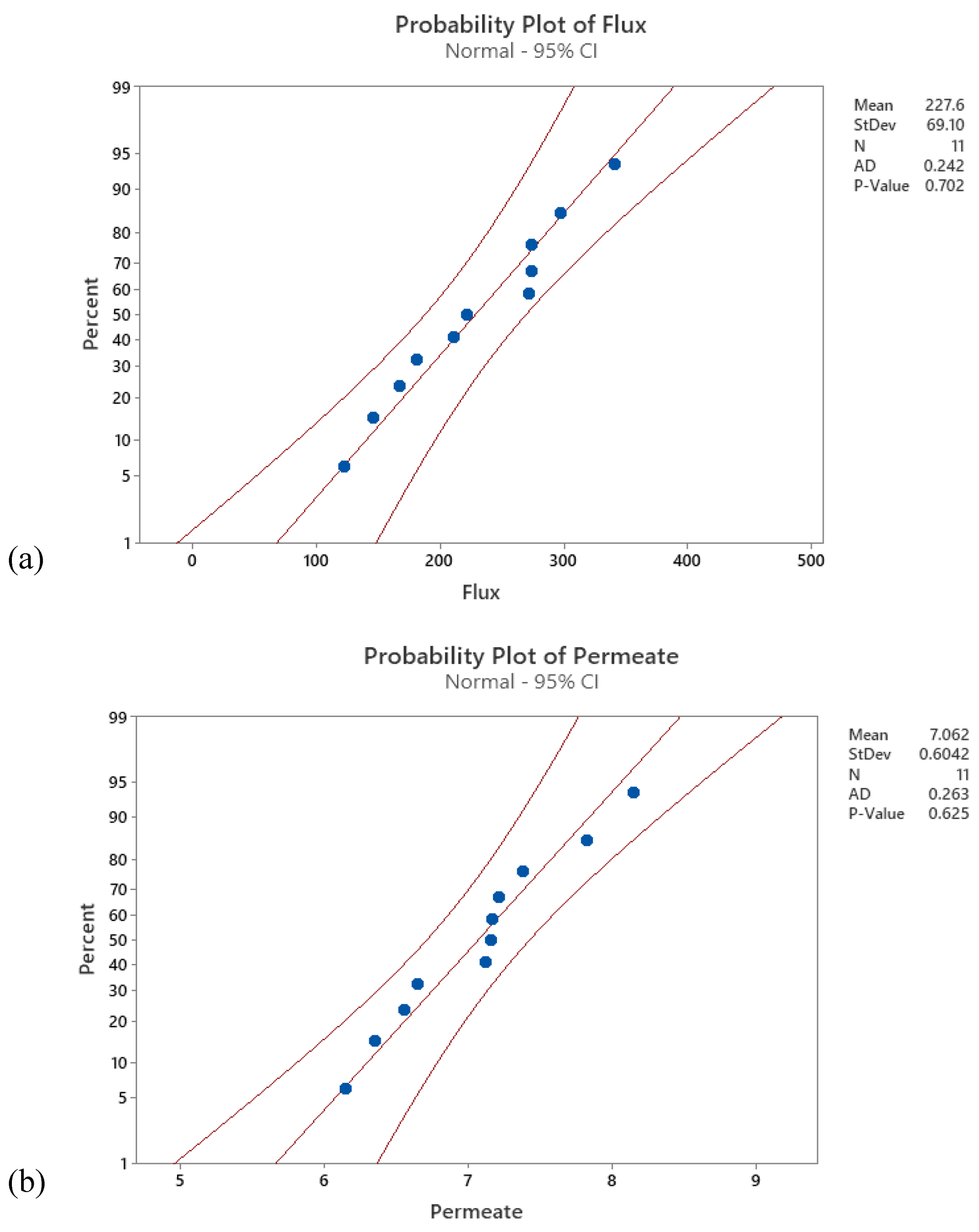
To provide statistical evidence of the model goodness of fit to predict the experimental data, a normal distribution of the collected data is assumed [71]. The mentioned assumption can be verified using one of the following statistical tests: Anderson-Darling Test, Ryan-Joiner Test, Shapiro-Wilk Test, Kolmogorov-Smirnov Test, Scatter Plot, or Normal Probability Plot. In this study, the normal probability plot (P-P) for membrane flux and permeate volume was performed at a CI of 95%, as depicted in Figure 5, respectively. A comparison between the P-value to the significance level (0.05) in the P-P plot indicates that the null hypothesis to reject the normality of the data fails (p-value > 0.05). There is insufficient evidence to conclude that the experimental data is not normally distributed. In addition, a visualization of the P-P plot reasonably indicates that all the data points are linearly close to the linear regression line and within the confidence interval of 95%. Therefore, the experimental data are normally distributed at a CI of 95%.
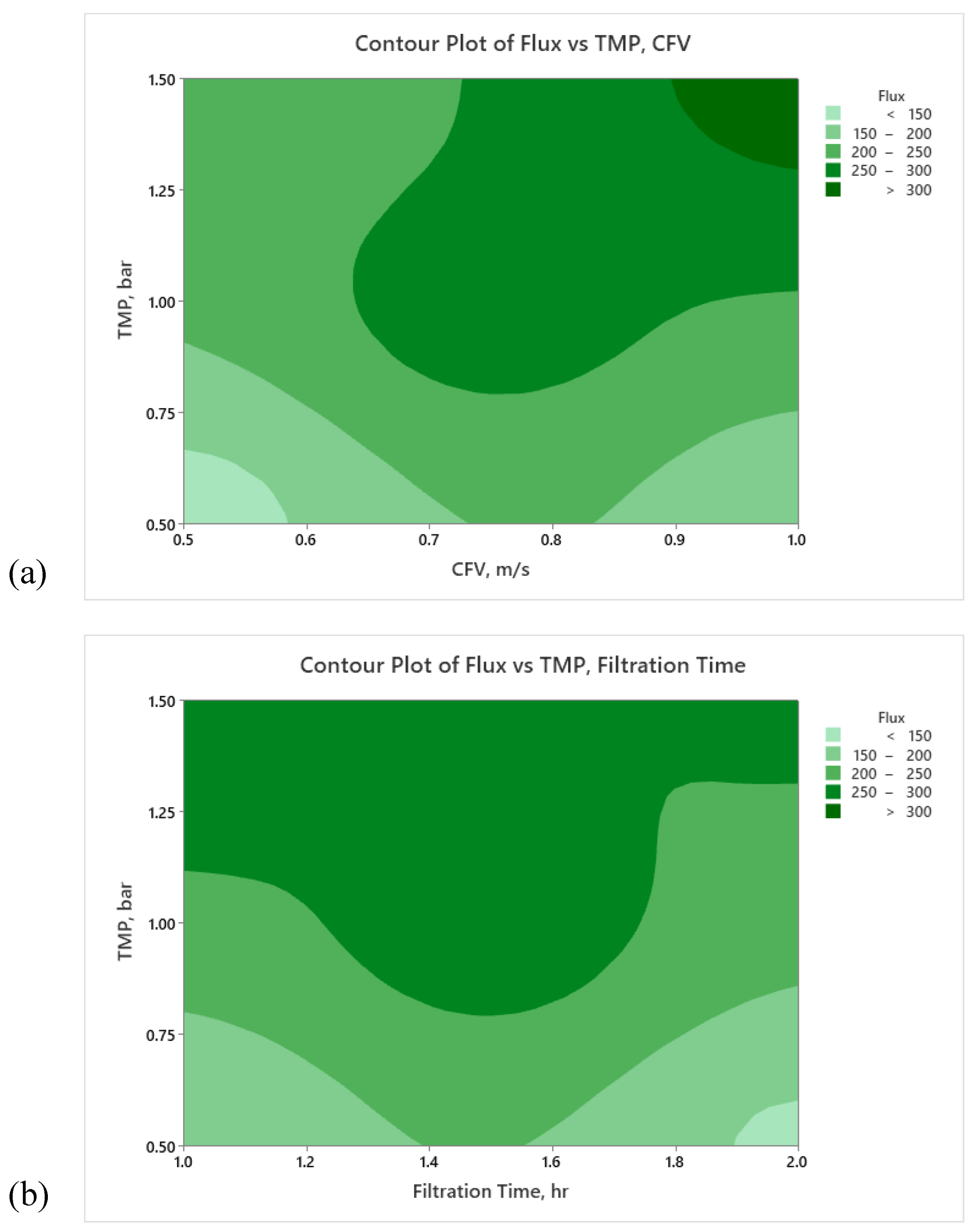
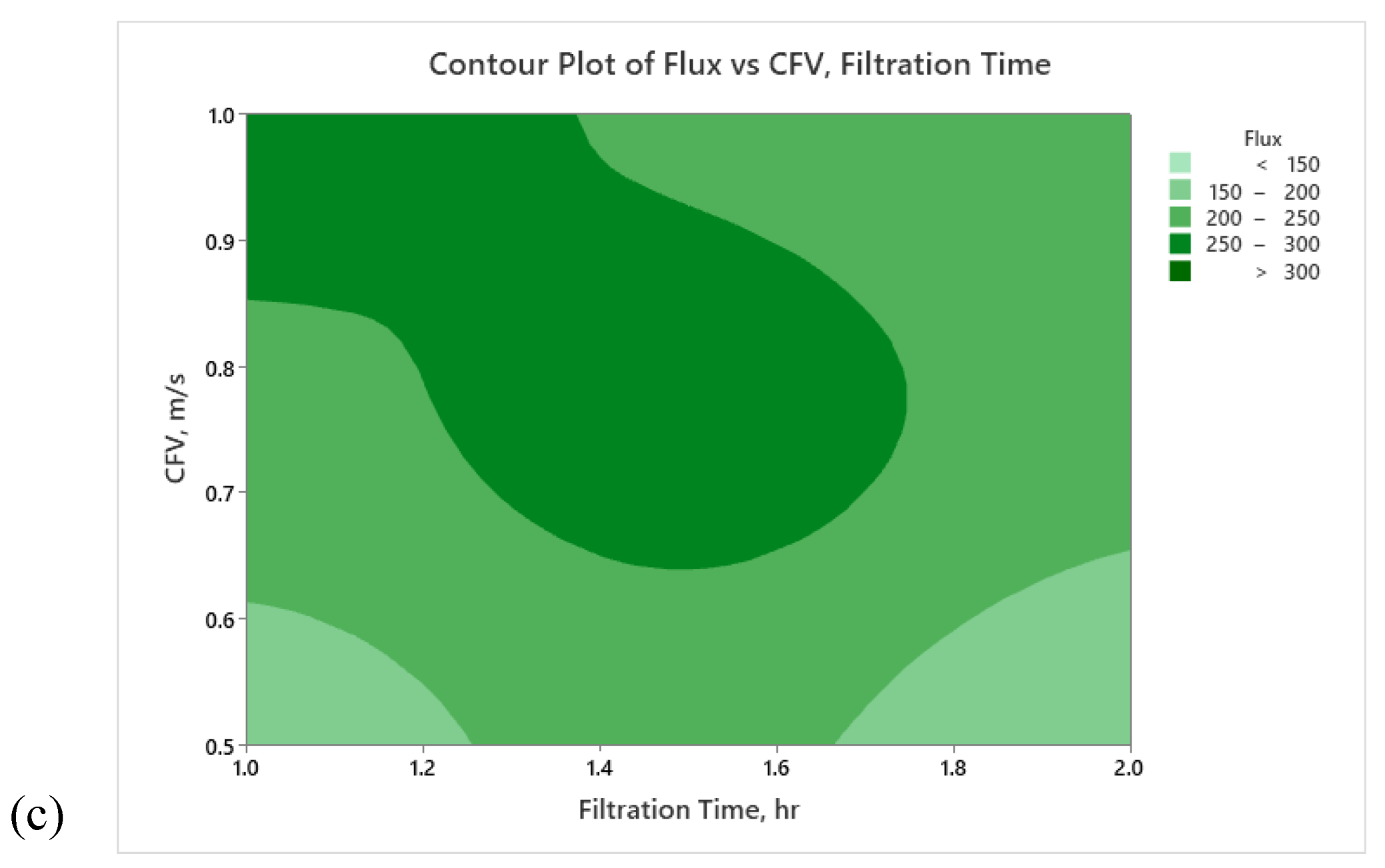
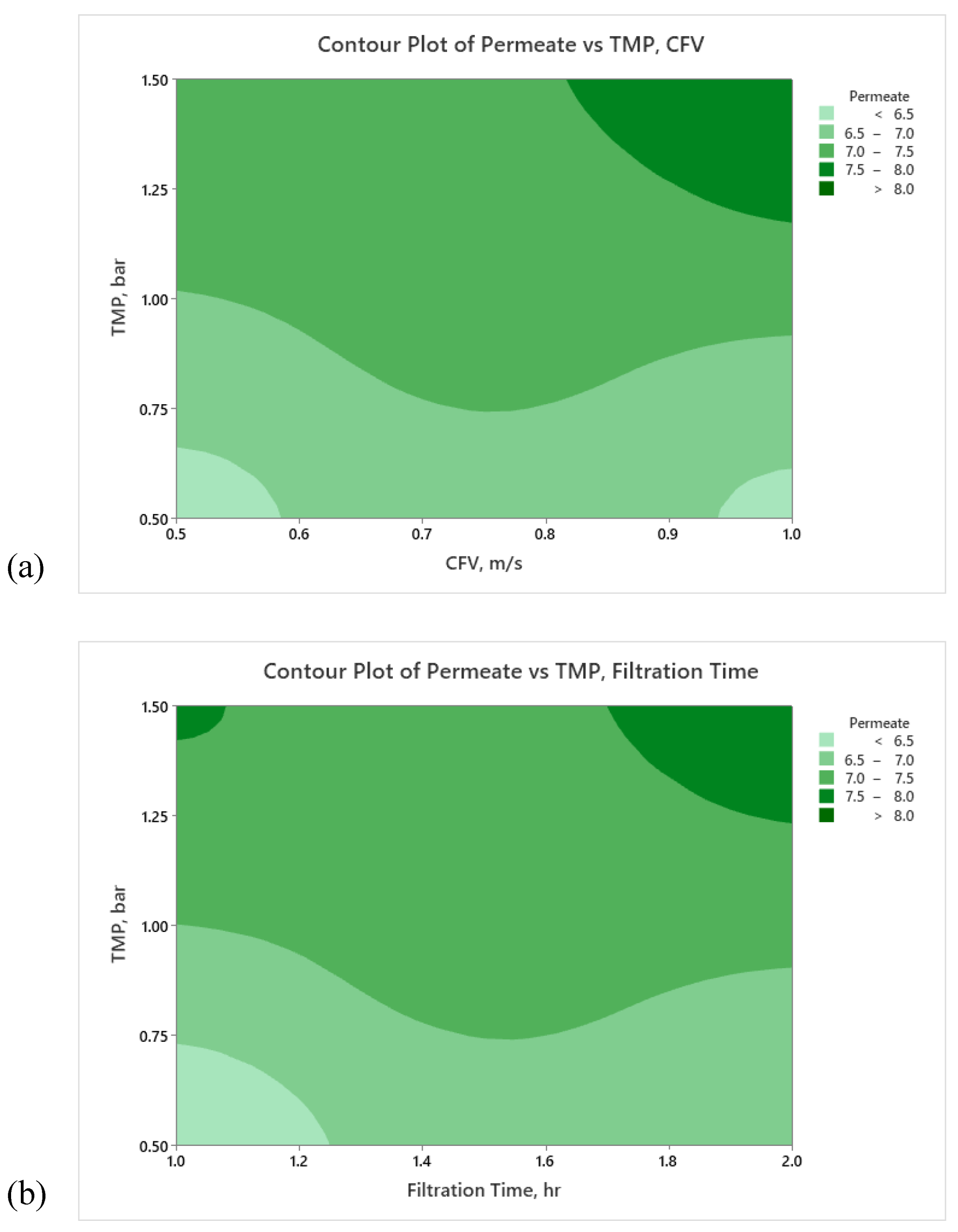
Figure 6 (a) and Figure 7(a) display the impact of the CFV and TMP on the membrane flux and permeate volume, respectively. From the plots contour, the flux and permeate volume are enhanced by increasing the TMP and CFV simultaneously.
The operation at the highest TMP of 1.5 bar (level +1) ensures a higher permeability due to the pressure-driven dragging permeation force of the feed toward the membrane surface. However, this is also associated with rapid oil droplets accumulation at/within the membrane pores, enhancing a concentration polarization barrier toward the continuous filtration process [72]. Coupling the TMP and CFV impacts the permeate flux, which appears to be enhanced with increasing CFV (to 1m/s) (Figure 6 (a)). Crossflow velocity creates turbulent hydrodynamic conditions at the membrane surface to boost cleaning by sweeping the oil droplets in the main crossflow field [73,74].
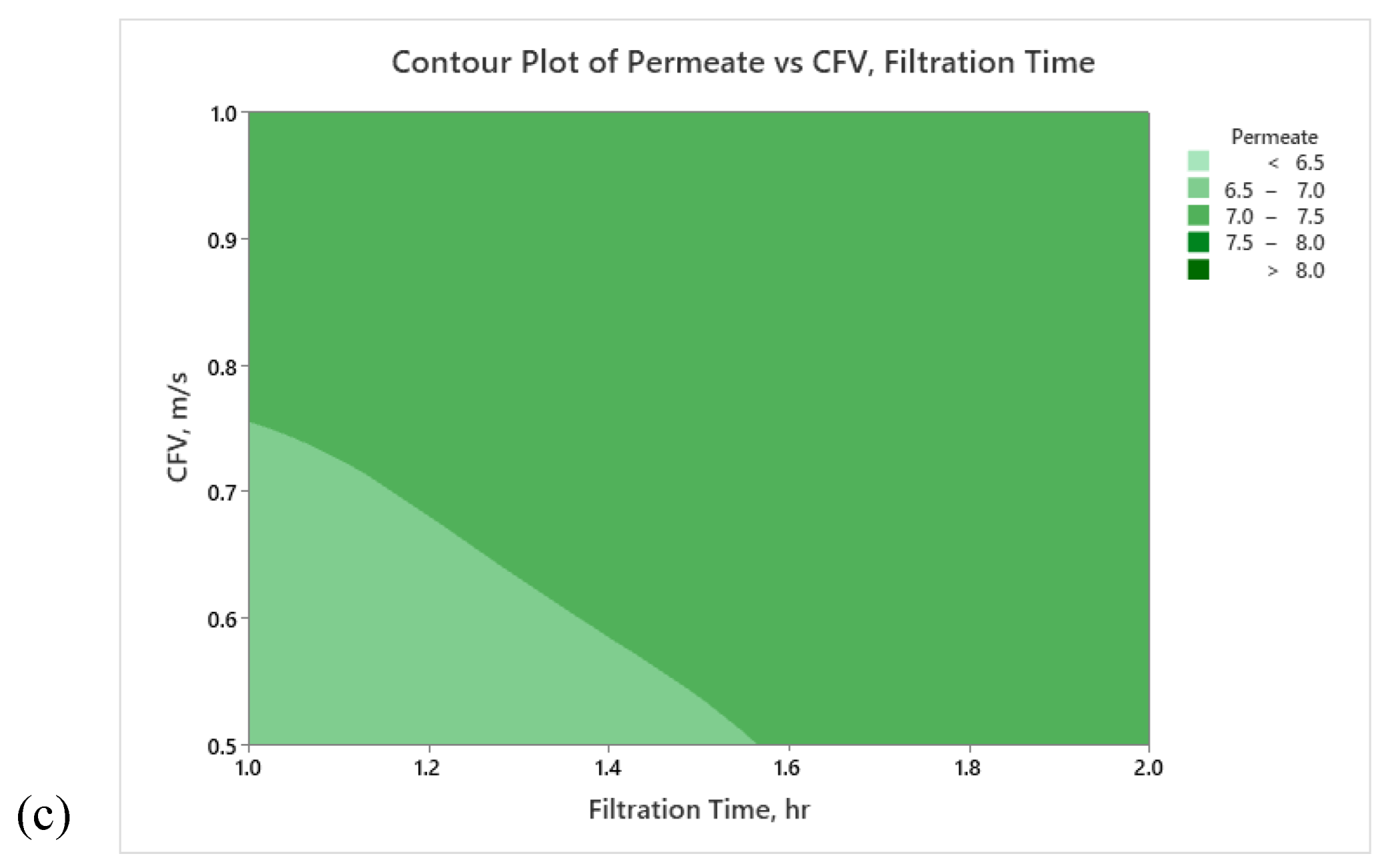
Figure 6 (c) shows that the membrane presents significant flux loss beyond one hour of operation. This is due to the formation of a fine cake layer of the accumulated oil droplets at the membrane surface. After one hour of operation, there is a hydrodynamic balance between the cleaning under the crossflow field and the accumulation and clustering of oil droplets at the membrane pores [8]. Figure 7 (c) depicted that the crossflow cleaning potential weakens beyond one hour and a half due to the fouling development and additional cake layer resistance in the membrane filtration system.
Figure 6 (b) and Figure 7(b) demonstrate no significant impact of the interaction of TMP and FT on the membrane flux and permeate volume without considering the CFV. The effect of CFV is required to consider FT. As mentioned in the ANOVA results, the two-way interaction between TMP and filtration time is insignificant at a 95% CI. Similar results were observed for CFV and filtration time (Figure 7 c).

4.1.3. Model Optimization Analysis

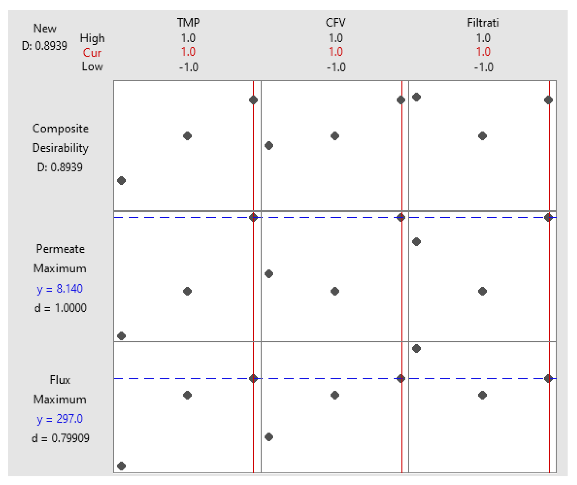
Model optimization settings were selected to increase the membrane’s final steady flux and permeate volume by determining the best operating conditions (TMP, CFV, and FT) (Table 11). TMP, CFV, and FT were set within their ranges. A multiple response prediction was performed to identify the two solutions (+1, +1, -1) and (+1, +1, +1) for maximum steady flux and permeate volume of 341 LMH and 7.82 L and 297 LMH and 8.14 L for a composite desirability function of 0.916 and 0.894, respectively (Table 12). The two selected configurations of the operating conditions were similar (TMP of 1.5 bar and CFV of 1m/s). The second solution is just a continuous process operation for an extra hour. For the process configuration (+1, +1, +1), the filtration time is 2 hours, the permeate volume is 8.14 L, and the final steady flux loss is 297 LMH. Operating at (+1, +1, +1) (Table 12) is characterized by an increase of permeate volume by 3.92% and a drop of the steady permeate flux by 12.90% compared to (+1, +1, -1). Operating the system beyond one hour shows more oil droplets accumulation at the membrane surface and a decline in the final permeate flux. In contrast, continuous filtration improves the overall permeate volume.
The selection of the best operating conditions can be based on the filtration time. The optimization plot (Figure 8) was used to identify the optimal operating configurations for the explanatory regressors, assuming the defined parameter accepted boundaries. The interactivity of the optimization plot eases the examination of the effect of the variables on the predicted responses. For this experiment design, the operating conditions (+1, +1, +1) were selected, prioritizing the permeate volume criterion while the steady flux level was still high and acceptable compared to (+1, +1, -1).
As a result, Full Factorial Design provides a structured and systematic approach to experimentally explore the effects of multiple factors on the filtration unit. It involves testing all possible combinations of factor levels. Full Factorial Design helps in understanding how different factors and their interactions affect the filtration process by providing insights into main effects and potential synergies or dependencies for pinpointing the most effective filtration parameters. Full Factorial Design focuses on identifying optimal conditions for the filtration process based on the observed data. It grants insights into which factor levels contribute most to desired outcomes. However, Full Factorial does not involve learning from data in the way AI techniques, especially machine learning (ML), do.
Rather than conducting a one-time Full Factorial experiment, a sequential approach can be adopted where AI is used to guide subsequent experiments based on the observed results, creating a dynamic and adaptive optimization process. Both AI techniques and Full Factorial Design can be used together for a comprehensive analysis. AI/ML can learn and analyze available data generated from experiments, providing additional insights and optimization opportunities.
When comparing AI and Full Factorial Design for a filtration system, it is important to recognize that these approaches serve different purposes and can be complementary in most situations. The following will explore how the machine learning method can be applied in the context of a filtration system.

4.2. MLR Analysis

Firstly, the MLR analysis method was performed to predict each of the eleven experimental runs. The results from the MLR analysis of all experimental data are summarised in Tables S1-S11. Nineteen training regression models were performed for each experiment, including linear regression models, regression trees, support vector machines, Gaussian process regression models, and ensembles of regression trees. For model training performance, the data were exported to the workspace, the features were selected, and validation schemes were specified fivefold. Then the performance was compared side-by-side using their R-squared, RMSE, MSE, and MAE statistical parameters. Tables S1-S11 displayed that the best model that describes all the experimental data for the eleven runs is the Gaussian regression process (GRP) with the Rational Quadratic training function. The Gaussian model presents the greatest R-squared and smallest RMSE, MSE, and MAE values, respectively. The validated model (GRP) results were diagnosticated for the eleven experiments for further analysis. The statistical performance of the model was measured using R-squared, RMSE, MSE, and MAE to see how well the model fitted the experimental data (Table 13). The results demonstrated a higher model’s goodness of fit to the data.
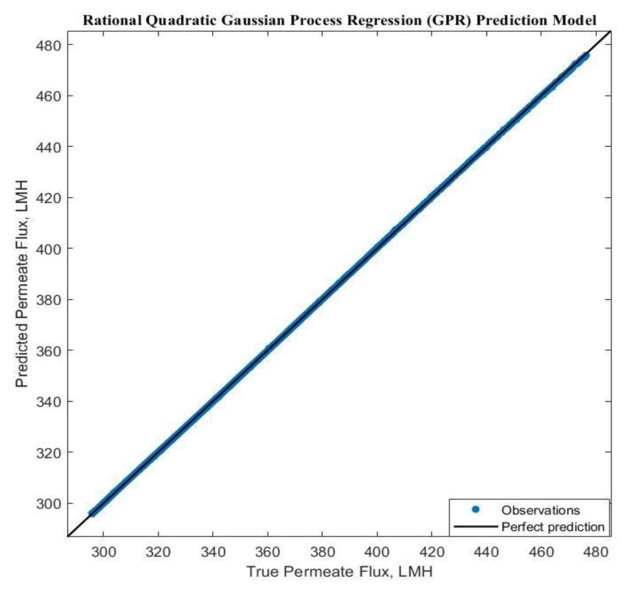
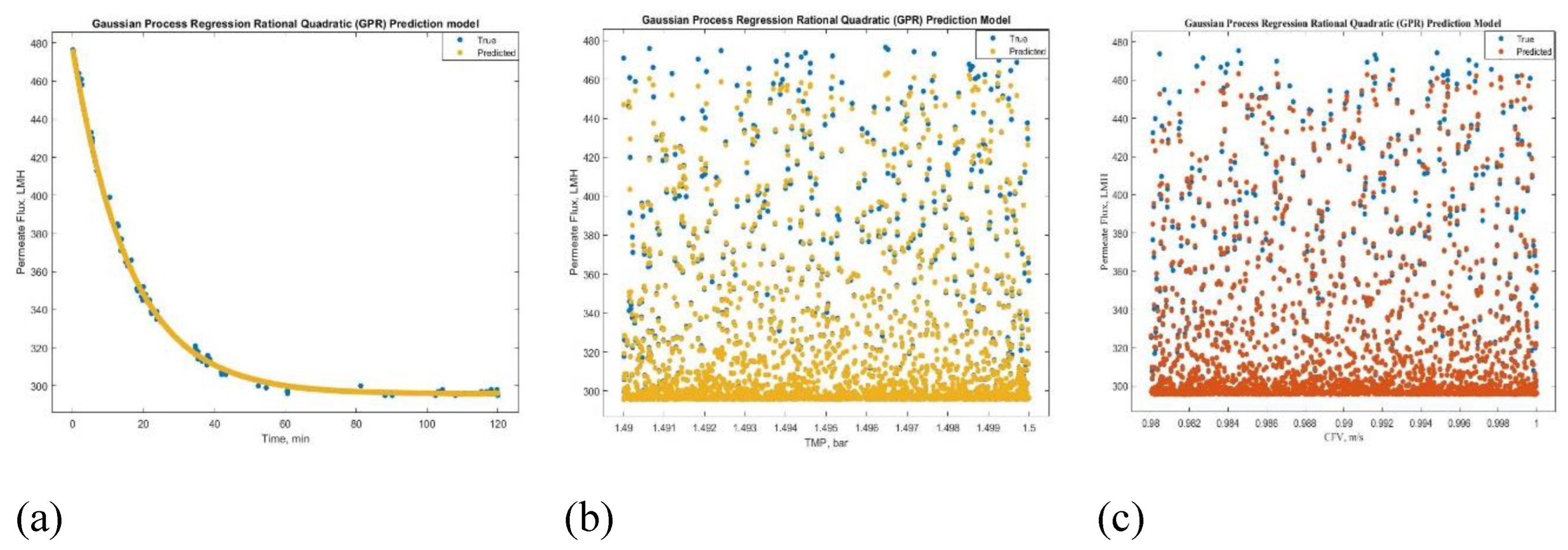
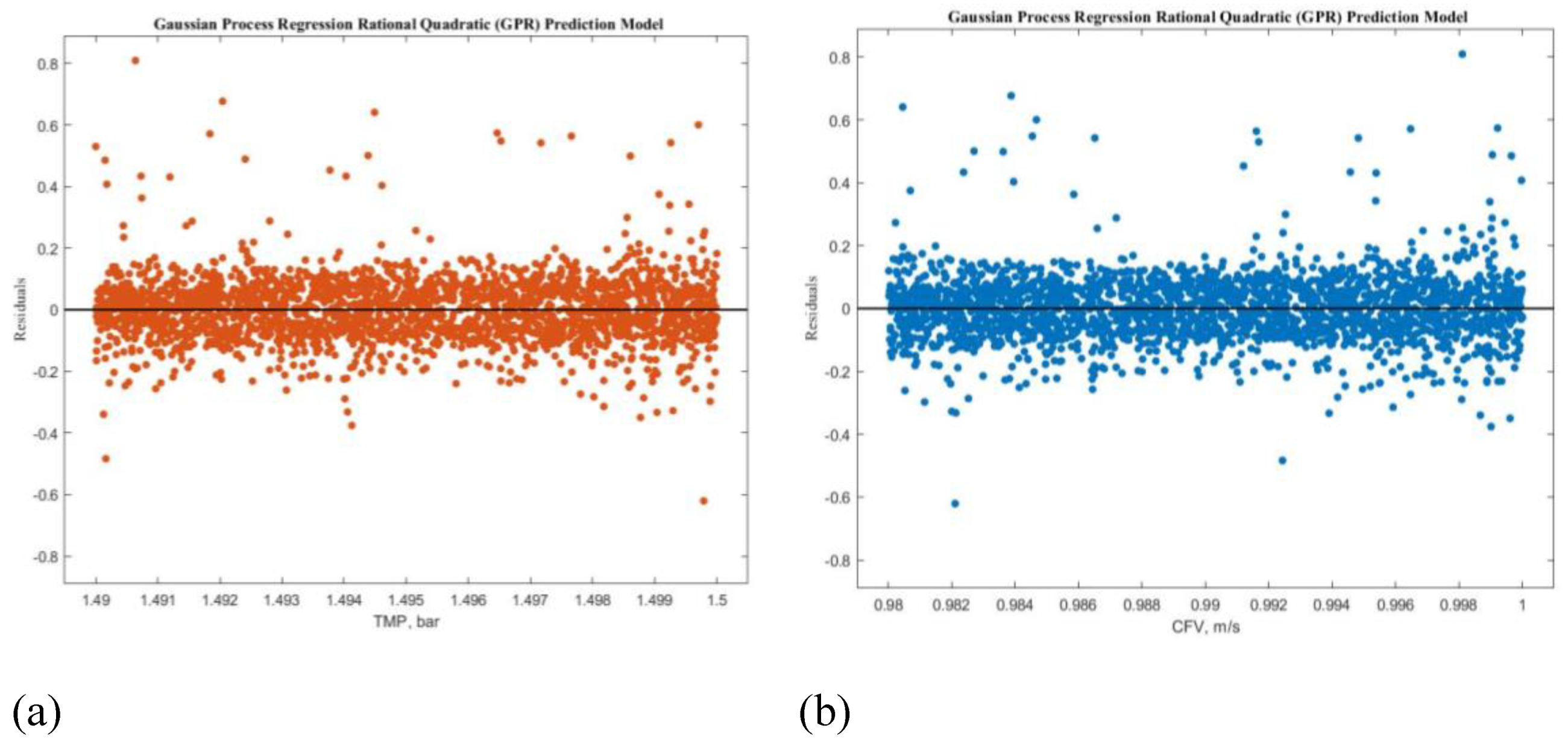
Experimental run #5 (+1, +1, +1) presented the best GRP model accuracy prediction performance. Additional diagnostic measures were performed to depict the model discrepancy between actual and expected values, such as the predicted versus actual plot (Figure 9). Furthermore, the response plots were analyzed to demonstrate the response fitted values as a function of experimental time (Figure 10 (a)), TMP (Figure 10 (b), and CFV (Figure 10 (c)), respectively. Figure 4.10 shows that the model accuracy is very high throughout the experimental time, aligning the actual and predicted results. The predicted permeate flux and the actual experimental data are error-zeroed at the steady stage filtration as a function of TMP or CFV, respectively. In contrast, the error at the early stage of filtration is very small due to the hydrodynamic environment of the filtration process (Figure 10 (b) and (c)). The residuals as a function of TMP and CFV were also plotted. Figure 11 (a),(b) show that the residuals are close to zero value for all TMP and CFV during the two hours of experiments, respectively.
In conclusion, the GRP model can predict 99% of the permeate flux for all the experimental runs (R-squared is 99% for all the trained models by the GRP algorithm). The GRP model is beneficial for estimating the membrane permeate flux when one or more operating conditions of the filtration system vary (TMP, CFV, and FT) without conducting any experimental run (Table 13). A screenshot of the optimization models is shown in Figures S5 and S6.

4.3. ANN Analysis

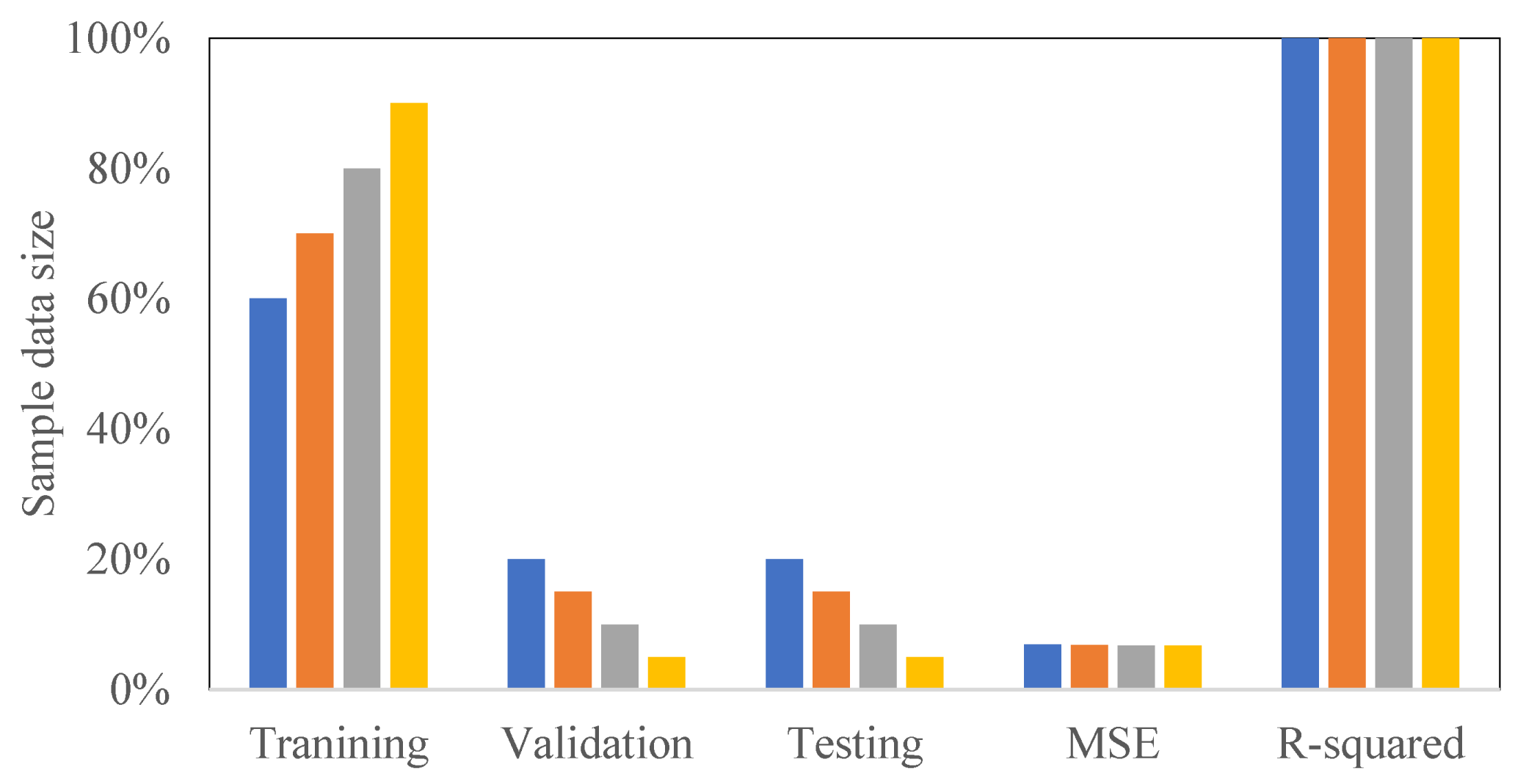
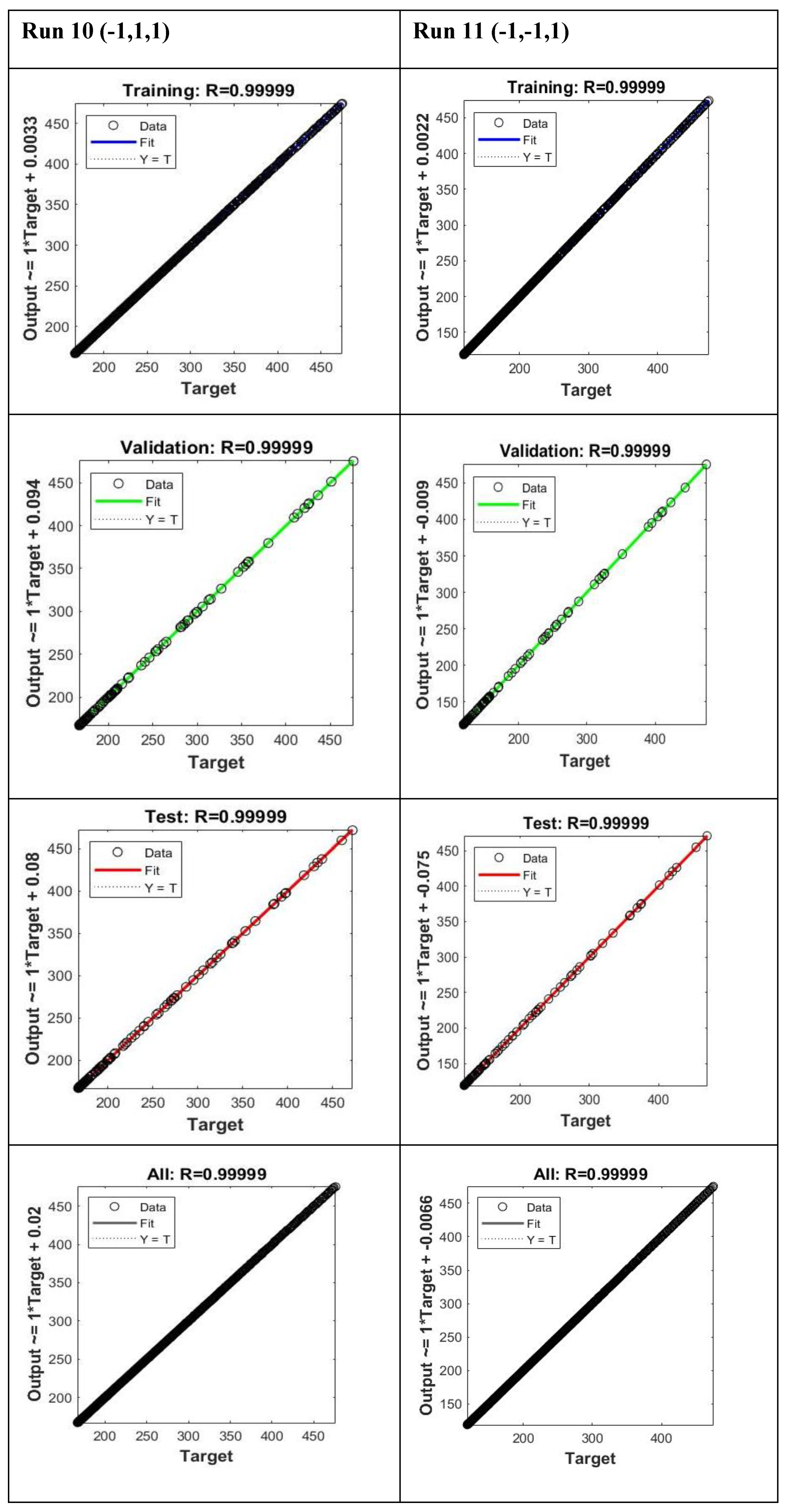
This study has also used an ANN modeling approach to predict the membrane permeate flux for the eleven experiments. ANN neural network training algorithm with the Levenberg-Marquardt (trainlm) backpropagation method was used to train all the data based on a feed-forward network with one hidden and output layer. Before the ANN analysis, the number of neurons in the hidden layer was optimized to select twenty neurons as the best-designed network. Additional analysis was performed to check the model performance against the training data percentage. Data were trained for 60, 70, 80, and 90% of the size of the experimental values to investigate its impact on the model correlation. Figure 12 demonstrates that the data percentage and the model training performance are not correlated. Table 14 demonstrates that the sample size depends on the filtration time. Sample sizes were 1200, 1800, and 2400 for a filtration time of one hour (level -1), one hour and a half (level 0), and two hours (level +1), respectively. The sample size was randomly divided for all experimental runs into 80% for training, 10% for validation, and 10% for testing. For experimental runs #2, 3, 6, and 9, 80% (960 samples) were randomly chosen for training, 10% (120 samples) for validation, and 10% (120 samples) for testing. For runs #1, 4, and 8, 80% (1440 samples) were arbitrarily designated for training, 10% (180 samples) for validation, and 10% (180 samples) for testing. For runs #5, 7, 10, and 11, 80% (1920 samples) were similarly selected for training, 10% (240 samples) for validation, and 10% (240 samples) for testing. The eleven overall models’ performances were analyzed using the Mean Squared Error (MSE) and correlation coefficient (R-value) and the results were summarized in Table 14.
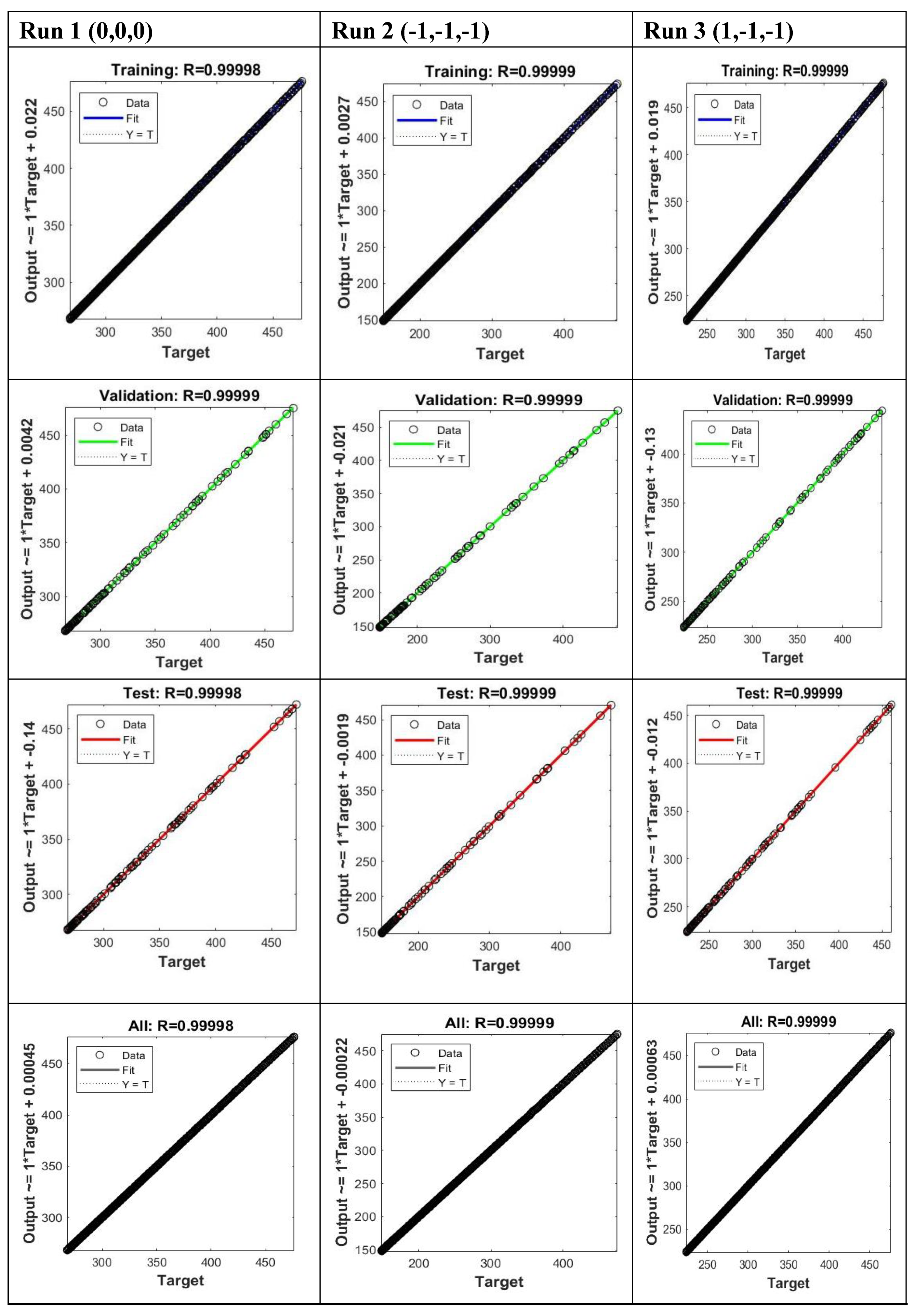
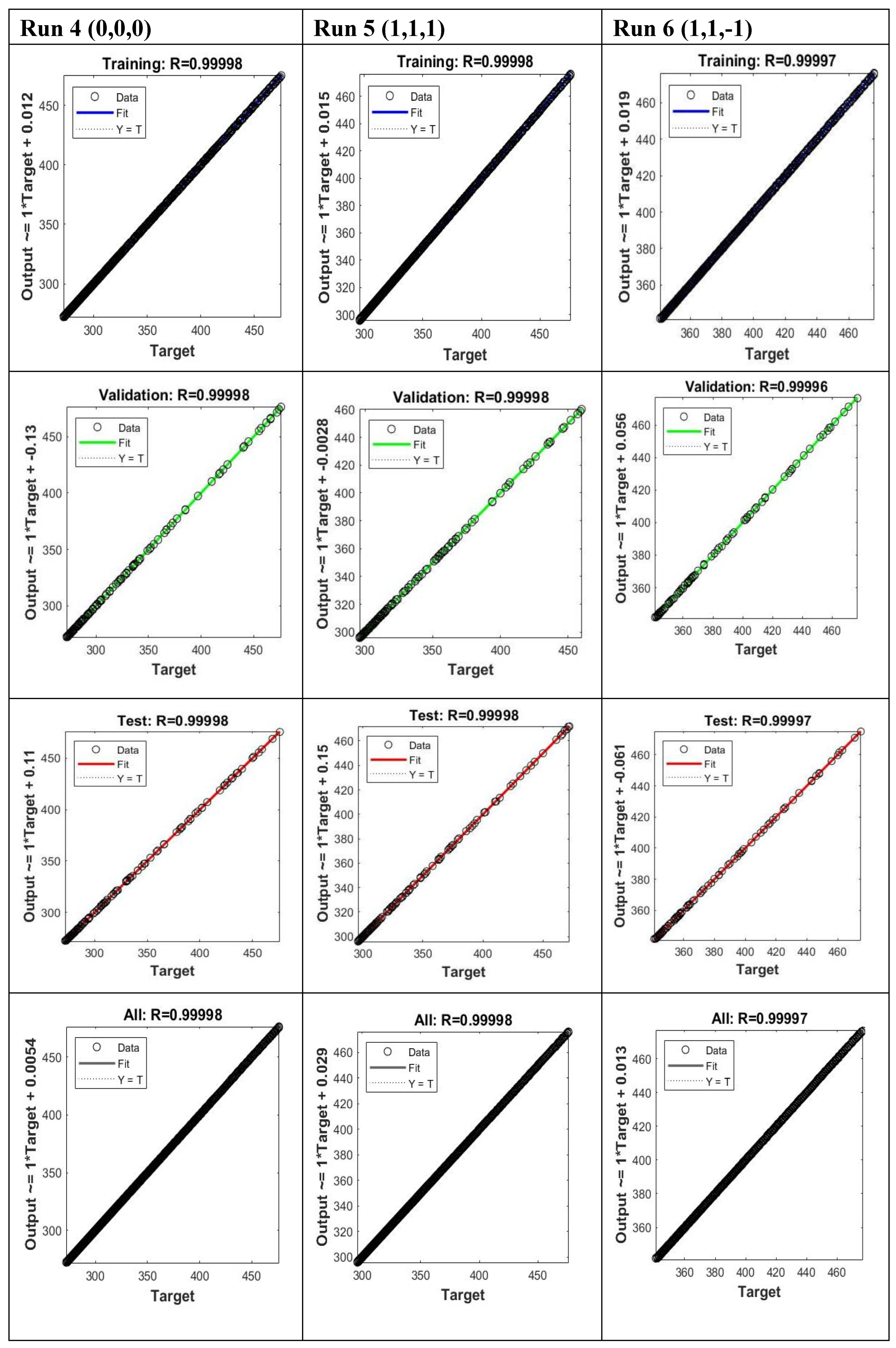
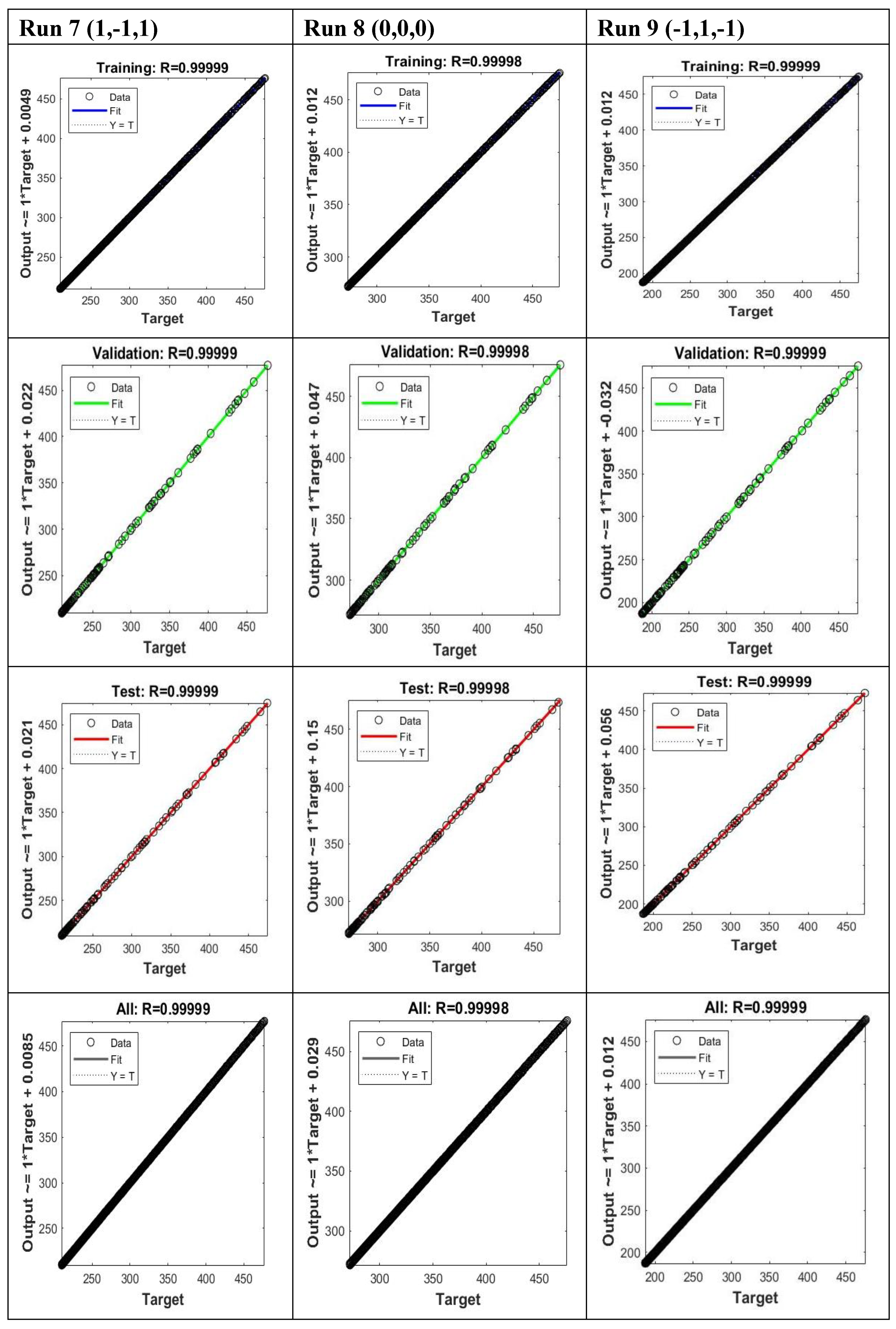
Figure 13 presents the training, validation, testing, and the overall ANN model’s linear correlation between the experimental data and model estimated values for the eleven experiments. Table 14 illustrates the correlation coefficient and the mean squared error of the ANN model for each experimental run. The results show that the regression line of all training models depicted a slope of one and an intercept of almost zero, indicating a strong agreement between the prediction and experimental data. In conclusion, the established ANN regression model performed at a goodness of fit of 99%. The model’s significant correlation can predict the experimentally collected data of the membrane permeate flux when the value of one or more operating conditions varies. Overall, the ANN design experiment technique has shown to be an eminent cost-effective approach to design, test, and improve the membrane filtration system performance for oily wastewater treatment.

5. Conclusion

In the present study, synthesized produced water from the Bakken reservoir in southern Saskatchewan (Canada) with an average feed-oil content of ~200 ppm was treated using an ultrafiltration titania ceramic membrane with a molecular weight cutoff of 150 kg/mol. The UF membrane demonstrated a superior rejection rate of oil droplets between 91% and 99% for all operating conditions of the eleven experiments. First, a full factorial design experiment examined the influence of the operating conditions (TMP, CFV, and FT) on the membrane permeate flux drop and permeate volume decline.
The best membrane performance was achieved at a TMP of 1.5 bar (level +1) and CFV of 1m/s (level +1) for a filtration time of one or two hours (level -1 or +1). The operating conditions were optimized for (+1, +1, +1) for a higher permeate volume of 8.14 L and steady permeate flux of 297 LMH, which is less than a 38% flux decline of the initial flux. To illustrate the effect of operational variables (TMP, CFV, and FT) and their interactions on membrane filtration efficiency and fouling alleviation. Analysis of Variance (ANOVA) was applied to analyze the outcomes of the full factorial design experiment. For CI of 95%, two empirical regression models, flux and permeate volume, were presented with a goodness of fit at 99.99% and 99.98% to predict the response values. The analysis of primary operating conditions and their interaction effects indicated as follows: (a) for membrane flux: TMP > CFV > (TMP × CFV) > FT > (TMP × CFV × FT) > (CFV × FT), and for permeate volume (b): TMP > CFV > (TMP× CFV) > FT > (TMP × CFV × FT).
Two model predictive approaches were used namely the multiple linear regression (MLR) model and the ANN technique. In the MLR analysis, nineteen training regression algorithms were tested for each of the eleven experimental runs, involving Linear regression models, Regression trees, Support vector machines, Gaussian process regression models, and Ensembles of regression trees. The models’ performance indexes were compared using statistical parameters such as R-squared, RMSE, MSE, and MAE to select the best algorithm to predict the experimental data. Gaussian regression process (GRP) with the Rational Quadratic training function was identified as the best multiple linear regression model to estimate the permeate flux for all the experiments. Note that there is a satisfactory agreement between the GRP model predicted values with the collected experimental data.
ANN neural network training algorithm with a backpropagation method Levenberg-Marquardt was tested to train all the eleven sets of experimental data at each operating condition based on a feed-forward network of one hidden layer of 20 neurons and one output layer. ANN modeling approach was applied to approximate the final steady membrane permeate flux. The ANN-trained model was found to be a cost-effective approach to optimizing and improving the UF membrane performance by predicting the steady flux decline during the experiment. The optimized performance achieved a coefficient of determination of 99% and a mean squared error of 0.067.

Supplementary Materials

The following supporting information can be downloaded at the website of this paper posted on Preprints.org. Figure S1: Multiple linear regression models, Figure S2. Machine learning flux regression models analysis, Figure S3. Ceramic membrane dimensions: (a) the complete illustration, (b) cross-sectional area, (c) ceramic membrane internal channels and walls, Figure S4. Contact angles of a Bakken oil droplet at the ceramic membrane surface, Figure S5. Contact angles of a water droplet at the ceramic membrane surface, Figure S6. LabBrain crossflow ceramic membrane filtration unit, Figure S7. LabBrain P&I control loop schematic diagram unit; Table S1. Algorithms models and their training functions fitted for the experimental run 1, Table S2. Algorithms models and their training functions fitted for the experimental run 2, Table S3. Algorithms models and their training functions fitted for the experimental run 3, Table S4. Algorithms models and their training functions fitted for the experimental run 4, Table S5. Algorithms models and their training functions fitted for the experimental run 5, Table S6. Algorithm models and their training functions ions fitted for the experimental run 6, Table S7. Algorithms models and their training functions fitted for the experimental run 7, Table S8. Algorithms models and their training functions fitted for the experimental run 8, Table S9. Algorithms models and their training functions fitted for the experimental run 9, Table S10. Algorithms models and their training functions fitted for the experimental run 10, Table S11. Algorithms models and their training functions fitted for the experimental run 11.

Author Contributions

M.E.: writing—original draft, writing—review and editing, data curation, investigation, methodology, and conceptualization; A.H.: formal analysis, review, editing, validation, supervision, funding, laboratory equipment, and chemicals; A.S.: review, editing, validation, and supervision. All authors have read and agreed to the published version of the manuscript.

Funding

This work was supported by the Natural Sciences and Engineering Research Council of Canada (NSERC) with a Discovery Grant (RGPIN-2024-05070).

Institutional Review Board Statement

Not applicable.

Informed Consent Statement

Not applicable.

Data Availability Statement

All data are presented in the article.

Conflicts of Interest

The authors declare no conflict of interest.

Abbreviations

AI Artificial Intelligent
ANFIS Adaptive Neuro-Fuzzy Inference System
ANN Artificial Neural Networks
ANN-MPC ANN Model Predictive Control
ANOVA Analysis of Variance
BP Backpropagation
COD Chemical Oxygen Demand
GA Genetic Algorithm
GRNN General Regression Neural Network
MLR Multiple Linear Regression
MSE Mean Squared Error
RSM Response Surface Methodology
SVM Support Vector Machine
PLSR Partial least squares regression

Appendix A

Membrane Cleaning in Place Procedure

First, the filtration unit is drained from the produced water, and the reverse osmosis water is injected into the LabBrain unit to clean the fouled ceramic membrane in place for 15 minutes at 50 °C. Second, the membrane element is cleaned with Sodium hydroxide, NaOH (15-20g/L, 85°C, 30 minutes), and Phosphoric acid, H3PO4 (85%, 5ml/L, 50°C, 15 minutes). Third, reverse osmosis water was circulated for 15 minutes and flushed for a complete unit rinse until neutrality was reached. Then, the permeability test, using deionized water, was performed to measure the ceramic membrane’s regeneration level. The regeneration was repeated until 99% of the initial permeate flux was attained.

References

  1. Echakouri, M.; Salama, A.; Henni, A. Experimental Investigation of the Novel Periodic Feed Pressure Technique in Minimizing Fouling during the Filtration of Oily Water Systems Using Ceramic Membranes. Membranes 2022, 12, 868. [Google Scholar] [CrossRef]
  2. Zoubeik, M.; Echakouri, M.; Henni, A.; Salama, A. Taguchi Optimization of Operating Conditions of a Microfiltration Alumina Ceramic Membrane and Artificial Neural-Network Modeling. J. Environ. Eng. 2022, 148, 4022001. [Google Scholar] [CrossRef]
  3. Echakouri, M.; Zoubeik, M.; Salama, A.; Henni, A.; Elgharbi, H. Recent Advances in the Physical Methods to Combat Membrane Fouling: An Emphasis on the Periodic Feed Pressure Technique. Sustain. Energy-Water-Environment Nexus Deserts 2022, 197–207. [Google Scholar]
  4. Echakouri, M.; Henni, A.; Salama, A. High-Frequency Pulsatile Parameterization Study for the Titania Ceramic Membrane Fouling Mitigation in Oily Wastewater Systems Using the Box–Behnken Response Surface Methodology. Membranes 2022, 12, 1198. [Google Scholar] [CrossRef] [PubMed]
  5. Fonseca Ivo, O.; Imsland, L.S. Framework for produced water discharge management with flow-weighted mean concentration based economic model predictive control. Comput. Chem. Eng. 2022, 157, 107604. [Google Scholar]
  6. Obotey Ezugbe, E.; Rathilal, S. Membrane technologies in wastewater treatment: A review. Membranes 2020, 10, 89. [Google Scholar] [CrossRef]
  7. Suhalim, N.S.; Kasim, N.; Mahmoudi, E.; Shamsudin, I.J.; Mohammad, A.W.; Mohamed Zuki, F.; Jamari, N.L.A. Rejection Mechanism of Ionic Solute Removal by Nanofiltration Membranes: An Overview. Nanomaterials 2022, 12, 437. [Google Scholar] [CrossRef] [PubMed]
  8. Echakouri, M.; Salama, A.; Henni, A. Experimental and computational fluid dynamics investigation of the deterioration of the rejection capacity of the membranes used in the filtration of oily water systems. ACS ES&T Water 2021, 1, 728–744. [Google Scholar]
  9. Darowna, D.; Wróbel, R.; Morawski, A.W.; Mozia, S. The influence of feed composition on fouling and stability of a polyethersulfone ultrafiltration membrane in a photocatalytic membrane reactor. Chem. Eng. J. 2017, 310, 360–367. [Google Scholar] [CrossRef]
  10. Jang, D.; Lee, J.; Jang, A. Impact of pre-coagulation on the ceramic membrane process during oil-water emulsion separation: Fouling behavior and mechanism. Chemosphere 2023, 313, 137596. [Google Scholar] [CrossRef]
  11. Rey, C.; Hengl, N.; Baup, S.; Karrouch, M.; Dufresne, A.; Djeridi, H.; Dattani, R.; Pignon, F. Velocity, stress and concentration fields revealed by micro-PIV and SAXS within concentration polarization layers during crossflow ultrafiltration of colloidal Laponite clay suspensions. J. Memb. Sci. 2017, 578, 69–84. [Google Scholar] [CrossRef]
  12. Khan, H.; Khan, S.U.; Hussain, S.; Ullah, A. Modelling of transmembrane pressure using slot/pore blocking model, response surface and artificial intelligence approach. Chemosphere 2022, 290, 133313. [Google Scholar] [CrossRef]
  13. Zoubeik, M.; Henni, A. Ultrafiltration of oil-in-water emulsion using a 0.04 µm silicon carbide membrane: Taguchi experimental design approach. Desalin. Water Treat. 2017, 62, 108–119. [Google Scholar] [CrossRef]
  14. Zoubeik, M.; Salama, A.; Henni, A. A comprehensive experimental and artificial network investigation of the performance of an ultrafiltration titanium dioxide ceramic membrane: Application in produced water treatment. Water Environ. J. 2019, 33, 459–4759. [Google Scholar] [CrossRef]
  15. Zoubeik, M.; Salama, A.; Henni, A. Table Optimization of Operating Conditions for a Superwetting Ultrafiltration ZrO2 Ceramic Membrane. J. Environ. Eng. 2020, 146, 4020021. [Google Scholar] [CrossRef]
  16. Aloulou, H.; Attia, A.; Aloulou, W.; Chakraborty, S.; Baklouti, L.; Dammak, L.; Amar, R.B. Statistical Simulation, a Tool for the Process Optimization of Oily Wastewater by Crossflow Ultrafiltration. Membranes 2022, 12, 676. [Google Scholar] [CrossRef] [PubMed]
  17. Louhıchı, G.; Bousselmı, L.; Ghrabı, A.; Khounı, I. Process optimization via response surface methodology in the physico-chemical treatment of vegetable oil refinery wastewater. Environ. Sci. Pollut. Res. 2019, 26, 18993–19011. [Google Scholar] [CrossRef] [PubMed]
  18. Šereš, Z.; Maravić, N.; Takači, A.; Nikolić, I.; Šoronja-Simović, D.; Jokić, A.; Hodur, C. Treatment of vegetable oil refinery wastewater using alumina ceramic membrane: Optimization using response surface methodology. J. Clean. Prod. 2016, 112, 3132–3137. [Google Scholar] [CrossRef]
  19. Khalifa, O.; Banat, F.; Srinivasakannan, C.; AlMarzooqi, F.; Hasan, S.W. Ozonation-assisted electro-membrane hybrid reactor for oily wastewater treatment: A methodological approach and synergy effects. J. Clean. Prod. 2021, 289, 125764. [Google Scholar] [CrossRef]
  20. Popović, S.; Karadžić, M.; Cakl, J. Optimization of ultrafiltration of cutting oil wastewater enhanced by application of twisted tapes: Response surface methodology approach. J. Clean. Prod. 2019, 231, 320–330. [Google Scholar] [CrossRef]
  21. Ruby-Figueroa, R.; Nardi, M.; Sindona, G.; Conidi, C.; Cassano, A. A multivariate statistical analyses of membrane performance in the clarification of citrus press liquor. ChemEngineering 2019, 3, 10. [Google Scholar] [CrossRef]
  22. Vyas, A.D.; Bennett, R.J.; Marshall, A.D. Influence of operating conditions on membrane fouling in crossflow microfiltration of particulate suspensions. Int. Dairy J. 2000, 10, 477–487. [Google Scholar] [CrossRef]
  23. De Almeida, M.S.; Martins, R.C.; Quinta-Ferreira, R.M.; Gando-Ferreira, L.M. Optimization of operating conditions for the valorization of olive mill wastewater using membrane processes. Environ. Sci. Pollut. Res. 2018, 25, 21968–21981. [Google Scholar] [CrossRef] [PubMed]
  24. Haddaji, C.; Ennaciri, K.; Driouich, A.; Digua, K.; Souabi, S. Optimization of the coagulation-flocculation process for vegetable oil refinery wastewater using a full factorial design. Process Saf. Environ. Prot. 2022, 160, 803–816. [Google Scholar] [CrossRef]
  25. Xu, Q.; Xu, Y.; Li, L.; Fang, K. Uniform experimental design in chemometrics. J. Chemom. 2018, 32, e3020. [Google Scholar] [CrossRef]
  26. Corbatón-Báguena, M.J.; Vincent-Vela, M.C.; Gozálvez-Zafrilla, J.M.; Álvarez-Blanco, S.; Lora-García, J.; Catalán-Martínez, D. Comparison between artificial neural networks and Hermia’s models to assess ultrafiltration performance. Sep. Purif. Technol. 2016, 170, 434–444. [Google Scholar] [CrossRef]
  27. Merma, A.G.; Santos, B.F.; Rego, A.S.; Hacha, R.R.; Torem, M.L. Treatment of oily wastewater from mining industry using electrocoagulation: Fundamentals and process optimization. J. Mater. Res. Technol. 2020, 9, 15164–15176. [Google Scholar] [CrossRef]
  28. Chen, Y.; Shen, L.; Li, R.; Xu, X.; Hong, H.; Lin, H.; Chen, J. Quantification of interfacial energies associated with membrane fouling in a membrane bioreactor by using BP and GRNN artificial neural networks. J. Colloid Interface Sci. 2020, 565, 1–10. [Google Scholar] [CrossRef] [PubMed]
  29. Chen, Y.; Yu, G.; Long, Y.; Teng, J.; You, X.; Liao, B.-Q.; Lin, H. Application of radial basis function artificial neural network to quantify interfacial energies related to membrane fouling in a membrane bioreactor. Bioresour. Technol. 2019, 293, 122103. [Google Scholar] [CrossRef]
  30. Waqas, S.; Harun, N.Y.; Sambudi, N.S.; Arshad, U.; Nordin, N.A.H.M.; Bilad, M.R.; Saeed, A.A.H.; Malik, A.A. SVM and ANN Modelling Approach for the Optimization of Membrane Permeability of a Membrane Rotating Biological Contactor for Wastewater Treatment. Membranes 2022, 12, 821. [Google Scholar] [CrossRef]
  31. Yogarathinam, L.T.; Velswamy, K.; Gangasalam, A.; Ismail, A.F.; Goh, P.S.; Subramaniam, M.N.; Satya Narayana, M.; Yaacob, N.; Abdullah, M.S. Parametric analysis of lignocellulosic ultrafiltration in lab scale crossflow module using pore blocking and artificial neural network model. Chemosphere 2022, 286, 131822. [Google Scholar] [CrossRef]
  32. Irfan, M.; Waqas, S.; Arshad, U.; Khan, J.A.; Legutko, S.; Kruszelnicka, I.; Ginter-Kramarczyk, D.; Rahman, S.; Skrzypczak, A. Response Surface Methodology and Artificial Neural Network Modelling of Membrane Rotating Biological Contactors for Wastewater Treatment. Materials 2022. 15, 1932. [CrossRef]
  33. Schmitt, F.; Banu, R.; Yeom, I.-T.; Do, K.-U. Development of artificial neural networks to predict membrane fouling in an anoxic-aerobic membrane bioreactor treating domestic wastewater. Biochem. Eng. J. 2018, 133, 47–58. [Google Scholar] [CrossRef]
  34. Jawad, J.; Hawari, A.H.; Zaidi, S.J. Modeling and sensitivity analysis of the forward osmosis process to predict membrane flux using a novel combination of neural network and response surface methodology techniques. Membranes 2021, 11, 70. [Google Scholar] [CrossRef] [PubMed]
  35. Ghaedi, A.M.; Ghaedi, M.; Pouranfard, A.R.; Ansari, A.; Avazzadeh, Z.; Vafaei, A.; Tyagi, I.; Agarwal, S.; Gupta, V.K. Adsorption of Triamterene on multi-walled and single-walled carbon nanotubes: Artificial neural network modeling and genetic algorithm optimization. J. Mol. Liq. 2016, 216, 654–665. [Google Scholar] [CrossRef]
  36. Ibrahim, S.; Wahab, N.A.; Ismail, F.S.; Sam, Y.M. Optimization of artificial neural network topology for membrane bioreactor filtration using response surface methodology. IAES Int. J. Artif. Intell. 2020, 9, 117. [Google Scholar] [CrossRef]
  37. Pendashteh, A.R.; Fakhru’l-Razi, A.; Chaibakhsh, N.; Abdullah, L.C.; Madaeni, S.S.; Abidin, Z.Z. Modeling of membrane bioreactor treating hypersaline oily wastewater by artificial neural network. J. Hazard. Mater. 2011, 192, 568–575. [Google Scholar] [CrossRef]
  38. Xu, H.; Xiao, K.; Yu, J.; Huang, B.; Wang, X.; Liang, S.; Wei, C.; Wen, X.; Huang, X. A simple method to identify the dominant fouling mechanisms during membrane filtration based on piecewise multiple linear regression. Membranes 2020, 10, 171. [Google Scholar] [CrossRef]
  39. Öztürk, O.B.; and Başar, E. Multiple linear regression analysis and artificial neural networks based decision support system for energy efficiency in shipping. Ocean Eng. 2022, 243, 110209. [Google Scholar] [CrossRef]
  40. Al Aani, S.; Bonny, T.; Hasan, S.W.; Hilal, N. Can machine language and artificial intelligence revolutionize process automation for water treatment and desalination? Desalination 2019, 458, 84–96. [Google Scholar] [CrossRef]
  41. Ullah, H.; Khan, I.; AlSalman, H.; Islam, S.; Asif Zahoor Raja, M.; Shoaib, M.; Gumaei, A.; Fiza, M.; Ullah, K.; Mizanur Rahman, S.M.; et al. Levenberg–Marquardt backpropagation for numerical treatment of micropolar flow in a porous channel with mass injection. Complexity 2021, 2021, 5337589. [Google Scholar] [CrossRef]
  42. Tang, S.Z.; Li, M.J.; Wang, F.L.; He, Y.L.; Tao, W.Q. Fouling potential prediction and multi-objective optimization of a flue gas heat exchanger using neural networks and genetic algorithms. Int. J. Heat Mass Transf. 2020, 152, 119488. [Google Scholar] [CrossRef]
  43. Monfared, M.A.; Kasiri, N.; Mohammadi, T. A CFD model for prediction of critical electric potential preventing membrane fouling in oily wastewater treatment. J. Memb. Sci. 2017, 539, 320–328. [Google Scholar] [CrossRef]
  44. Jang, H.; Park, S.-J.; Kim, J. Response surface methodology to investigate the effects of operational parameters on membrane fouling and organic matter rejection in hard-shell encased hollow-fiber membrane. Chemosphere 2022, 287, 132132. [Google Scholar] [CrossRef] [PubMed]
  45. Hakim, M.L.; Nugroho, B.; Suastika, I.K.; Utama, I.K.A.P. Alternative Empirical Formula for Predicting the Frictional Drag Penalty due to Fouling on the Ship Hull using the Design of Experiments (DOE) Method. Int. J. Technol. 2021, 12, 829–842. [Google Scholar] [CrossRef]
  46. Li, L.; Rong, S.; Wang, R.; Yu, S. Recent advances in artificial intelligence and machine learning for nonlinear relationship analysis and process control in drinking water treatment: A review. Chem. Eng. J. 2021, 405, 126673. [Google Scholar] [CrossRef]
  47. Viet, N.D.; Jang, D.; Yoon, Y.; Jang, A. Enhancement of membrane system performance using artificial intelligence technologies for sustainable water and wastewater treatment: A critical review. Crit. Rev. Environ. Sci. Technol. 2022, 52, 3689–3719. [Google Scholar] [CrossRef]
  48. Jawad, J.; Hawari, A.H.; Zaidi, S.J. Artificial neural network modeling of wastewater treatment and desalination using membrane processes: A review. Chem. Eng. J. 2021, 419, 129540. [Google Scholar] [CrossRef]
  49. Naghibi, S.A.; Salehi, E.; Khajavian, M.; Vatanpour, V.; Sillanpää, M. Multivariate data-based optimization of membrane adsorption process for wastewater treatment: Multilayer perceptron adaptive neural network versus adaptive neural fuzzy inference system. Chemosphere 2021, 267, 129268. [Google Scholar] [CrossRef]
  50. Belfort, G. Membrane filtration with liquids: A global approach with prior successes, new developments and unresolved challenges. Angew. Chemie 2019, 131, 1908–1918. [Google Scholar] [CrossRef]
  51. Kamali, M.; Appels, L.; Yu, X.; Aminabhavi, T.M.; Dewil, R. Artificial intelligence as a sustainable tool in wastewater treatment using membrane bioreactors. Chem. Eng. J. 2021, 417, 128070. [Google Scholar] [CrossRef]
  52. Park, S.; Baek, S.S.; Pyo, J.; Pachepsky, Y.; Park, J.; Cho, K.H. Deep neural networks for modeling fouling growth and flux decline during NF/RO membrane filtration. J. Memb. Sci. 2019, 587, 117164. [Google Scholar] [CrossRef]
  53. Mittal, S.; Gupta, A.; Srivastava, S.; Jain, M. Artificial Neural Network based modeling of the vacuum membrane distillation process: Effects of operating parameters on membrane fouling. Chem. Eng. Process. Intensif. 2021, 164, 108403. [Google Scholar] [CrossRef]
  54. Bagheri, M.; Akbari, A.; Mirbagheri, S.A. Advanced control of membrane fouling in filtration systems using artificial intelligence and machine learning techniques: A critical review. Process Saf. Environ. Prot. 2019, 123, 229–252. [Google Scholar] [CrossRef]
  55. Zhang, W.; Zhu, Z.; Jaffrin, M.Y.; Ding, L. Effects of hydraulic conditions on effluent quality, flux behavior, and energy consumption in a shear-enhanced membrane filtration using box-behnken response surface methodology. Ind. Eng. Chem. Res. 2014, 53, 7176–7185. [Google Scholar] [CrossRef]
  56. Myers, R.H.; Montgomery, D.C.; Vining, G.G.; Robinson, T.J. Robinson. In Generalized linear models: With applications in engineering and the sciences; John Wiley & Sons: Hoboken, NJ, USA, 2012. [Google Scholar]
  57. Fan, M.; Hu, J.; Cao, R.; Ruan, W.; Wei, X. A review on experimental design for pollutants removal in water treatment with the aid of artificial intelligence. Chemosphere 2018, 200, 330–343. [Google Scholar] [CrossRef] [PubMed]
  58. Khan, M.; Ahmad, I.; Ahsan, M.; Kano, M.; Caliskan, H. Prediction of optimum operating conditions of a furnace under uncertainty: An integrated framework of artificial neural network and genetic algorithm. Fuel 2022, 330, 125563. [Google Scholar] [CrossRef]
  59. Jawad, J.; Hawari, A.H.; Zaidi, S. Modeling of forward osmosis process using artificial neural networks (ANN) to predict the permeate flux. Desalination 2020, 484, 114427. [Google Scholar] [CrossRef]
  60. Gaudio, M.T.; Coppola, G.; Zangari, L.; Curcio, S.; Greco, S.; Chakraborty, S. Artificial intelligence-based optimization of industrial membrane processes. Earth Syst. Environ. 2021, 5, 385–398. [Google Scholar] [CrossRef]
  61. Phil, K. Matlab deep learning with machine learning, neural networks, and artificial intelligence; Apress: New York, 2017. [Google Scholar]
  62. Paluszek, M.; Thomas, S. Practical Matlab deep learning. A Proj. Approach, Michael Paluszek Stephanie Thomas, 2020. [Google Scholar]
  63. Viet, N.D.; Jang, A. Development of artificial intelligence-based models for the prediction of filtration performance and membrane fouling in an osmotic membrane bioreactor. J. Environ. Chem. Eng. 2021, 9, 105337. [Google Scholar] [CrossRef]
  64. Esfe, M.H.; Toghraie, D.; Amoozadkhalili, F. Optimization and design of ANN with Levenberg-Marquardt algorithm to increase the accuracy in predicting the viscosity of SAE40 oil-based hybrid nano-lubricant. Powder Technol. 2023, 415, 118097. [Google Scholar] [CrossRef]
  65. Giwa, A.; Daer, S.; Ahmed, I.; Marpu, P.R.; Hasan, S.W. Experimental investigation and artificial neural networks ANNs modeling of electrically-enhanced membrane bioreactor for wastewater treatment. J. Water Process Eng. 2016, 11, 88–97. [Google Scholar] [CrossRef]
  66. Paluszek, M.; Thomas, S. MATLAB machine learning recipes: A problem-solution approach; Apress, 2019. [Google Scholar]
  67. El Batouti, M.; Alharby, N.F.; Elewa, M.M. Review of New Approaches for Fouling Mitigation in Membrane Separation Processes in Water Treatment Applications. Separations 2021, 9, 1. [Google Scholar] [CrossRef]
  68. Zsirai, T.; Qiblawey, H.; Buzatu, P.; Al-Marri, M.; Judd, S.J. Cleaning of ceramic membranes for produced water filtration. J. Pet. Sci. Eng. 2018, 166, 283–289. [Google Scholar] [CrossRef]
  69. Weschenfelder, S.E.; Fonseca, M.J.C.; Costa, B.R.S.; Borges, C.P. Influence of the use of surfactants in the treatment of produced water by ceramic membranes. J. Water Process Eng. 2019, 32, 100955. [Google Scholar] [CrossRef]
  70. Kordkandi, S.A.; Forouzesh, M. Application of full factorial design for methylene blue dye removal using heat-activated persulfate oxidation. J. Taiwan Inst. Chem. Eng. 2014, 45, 2597–2604. [Google Scholar] [CrossRef]
  71. Montgomery, D.C. Design and analysis of experiments; John Wiley & sons, 2017. [Google Scholar]
  72. Hejase, C.A.; Tarabara, V.V. Nanofiltration of saline oil-water emulsions: Combined and individual effects of salt concentration polarization and fouling by oil. J. Memb. Sci. 2021, 617, 118607. [Google Scholar] [CrossRef]
  73. Salama, A.; Zoubeik, M.; Henni, A. A multicontinuum approach for the problem of filtration of oily water systems across thin flat membranes: I. The framework. AIChE J. 2017, 63, 4604–4615. [Google Scholar] [CrossRef]
  74. Salama, A.; Zoubeik, M.; Henni, A. A multicontinuum approach for the problem of filtration of oily-water systems across thin flat membranes: II. Validation and examples. AIChE J. 2018, 64, 1095–1105. [Google Scholar] [CrossRef]
Figure 1. Function fitting neural network view.
Preprints 114954 g001
Figure 2. Effect of the number of neurons in the ANN hidden layer on the model training performance.
Preprints 114954 g002
Figure 3. Pareto chart of the standardized effects of (a) the membrane flux and (b) permeate volume with a= 0.05.
Preprints 114954 g003
Figure 4. Factorial plots for (a) mean membrane flux and (b) permeate volume.
Preprints 114954 g004
Figure 5. Normal probability plots for (a) membrane flux and (b) permeate volume.
Preprints 114954 g005
Figure 6. Contour plots for membrane permeate flux as a function of (a) TMP and CFV, (b) TMP and FT, and (c) CFV and FT.
Preprints 114954 g006aPreprints 114954 g006b
Figure 7. Contour plots for permeate volume as a function of (a) TMP and CFV, (b) TMP and FT, and (c) CFV and FT.
Preprints 114954 g007aPreprints 114954 g007b
Figure 8. Optimization plot of the operating conditions. The dotes present the operating conditions levels (-1, 0, +1) for each factor (TMP, CFV, and FT).
Preprints 114954 g008
Figure 9. Predicted and real permeate flux correlation response plot.
Preprints 114954 g009
Figure 10. True and predicted permeate flux correlation as a function of (a) time, (b) TMP, and (c) CFV during the experiment.
Preprints 114954 g010
Figure 11. Normalized permeate flux residuals as a function of (a) TMP and (b) CFV for the experiment.
Preprints 114954 g011
Figure 12. Training performance (R-squared and MSE) as a function of the experimental data percentages training.
Preprints 114954 g012
Figure 13. ANN regression plots of the eleven experimental runs.
Preprints 114954 g013aPreprints 114954 g013bPreprints 114954 g013cPreprints 114954 g013d
Table 1. Overview of the operating conditions optimization design methods applied for the membrane processes.
Process Feed Operating conditions Response Optimization Methodology Performance Refs
Crossflow filtration unit (LiqTech) Produced water TMP, CFV, Temp, and pH Permeate flux Taguchi, ANOVA, and ANN Oil rejection= 98.25% [2]
Crossflow filtration unit (LiqTech) Produced water TMP, CFV, and pulsatile cycle Permeate flux and
Permeate volume
Box-Behnken, ANOVA 99% oil rejection, R2 = 99% [4]
Crossflow filtration unit (LiqTech) Produced water TMP, CFV, Temp, and pH Permeate flux fouling resistance Taguchi, ANOVA, and ANN 96% oil rejection [13]
Crossflow filtration unit (LiqTech) Produced water TMP, CFV, Temp, and pH Permeate flux Taguchi, ANOVA, and ANN 98.93% oil rejection
99% organic carbon removal (TOC)
99.82% turbidity removal
[14]
Crossflow filtration unit (LiqTech) Produced water TMP, CFV, Temp, and pH Permeate flux Taguchi, ANOVA, and ANN Oil rejection= 98%
Toral organic carbon= 99%
Turbidity rejection= 99%
[15]
Crossflow filtration unit industrial wastewater Oil concentration, TMP, Temp COD
Permeate flux
Box-Behnken, ANOVA COD removal, R = 0.985
Permeate flux, R = 0.901
[16]
Conventional jar-test apparatus Vegetable oil refinery Coagulant concentration, flocculent dosage, and
Initial pH
COD removal
Residual turbidity
Box-Behnken, ANOVA COD removal, R2 = 92.9%
Turbidity removal, R2 = 83.6%
[17]
Crossflow filtration unit Vegetable oil seed wastewater TMP, CFV, and Temp Permeate flux
Chemical oxygen demand reduction (%)
RSM COD removal enhanced from 40% to 75%. [18]
Ozonation-assisted hybrid reactor Oil and gas oily wastewater Hydraulic residence time, Aeration, Current density, Intermittent power, and initial pH COD rejection One-factor-at-a-time experimentation,
RSM
Efficiency was considerably improved, attaining 53.1% COD removal. [19]
Ultrafiltration crossflow filtration unit Cutting oil wastewater Oil content, CFV, TMP, aspect ratio, and (AR) of twisted tape Permeate flux
Energy consumption
Central composite face-centred design Maximal Steady flux= 201 LMH
Minimal specific energy consumption= 1.34 kWh/m3
[20]
Laboratory bench plant Orange press liquor Contact angle, membrane thickness, pore size distribution,
TMP, temperature, and
process time
Permeate flux, hesperidin, glucose, fructose, and sucrose rejection Partial least squares regression (PLSR) Permeate flux, R2 = 96.2%
Hesperidin rejection, R2 = 95.8%
Glucose rejection, R2 = 91.7%
Fructose rejection, R2 = 97.5%
Sucrose rejection, R2 = 94.3%
[21]
Double crossflow filtration unit (SEPA CF II - GE Osmonics) Olive mill wastewater TMP, Temp, and pH COD removal
Total phenolic removal
Full factorial design COD removal, R2 = 83.3%
Total phenolic removal, R2 = 93.1%
[23]
Refining operating unit Vegetable oil refineries wastewater pH, coagulant dose, flocculant dose, and pollutant load Turbidity
COD removal
Full factorial design, ANOVA analysis Turbidity, R = 0.96
COD removal, R = 0.9
[24]
Conventional crossflow pilot plant Polyethylene glycol (PEG) TMP, CFV, and time Permeate flux Hermia model and ANN Permeability, R² = 0.99 [26]
Flocculation and electrocoagulation laboratory unit Mining oily wastewater pH, current density, electrolyte concentration, oil concentration, and Electrode gap COD removal ANN, Polynomial GA Polynomial GA, R2= 0.89
ANN, R2= 0.99
[27]
Membrane rotating biological contactor Synthetic wastewater Disk Rotational Speed, hydraulic retention time, and sludge retention time Permeability SVM, ANN R2 = 99% [30]
Crossflow module (Rayflow 100 Plate and Frame Mode) Agricultural palm oily wastewater TMP, pH, and feed oil content Lignocellulosic permeate flux ANN, blocking laws Water recovery = 82 %
Rejection = 98%
[31]
Rotating biological contactors Food leftovers wastewater Disk rotational speed, membrane-to-disk gap, and organic loading rate Permeability RSM, ANN ANN, R2 = 0.9982
RSM, R2 = 0.9762
[32]
Anoxic-aerobic membrane bioreactor Domestic wastewater COD, MLSS, MLVSS, pH, DO, Alkalinity, TN, TP, NO3-N, and NH4-N Transmembrane pressure ANN R2 = 0.850 [33]
SEPA CF forward osmosis cell (Sterlitec) Distilled water or 0.086 M NaCl solution The osmotic pressure difference, feed solution (FS) velocity, draw solution (DS) velocity, and FS temperature, DS temperature Permeate flux RSM, ANN ANN, R2 = 0.98036
RSM, R2 = 0.9408
[34]
Batch experiment apparatus Drug solution pH, contact time, temperature
adsorbent dosage, and initial triamterene concentration
Naphthalene
removal efficiency
ANN-GA, MLR MSE = 0.0005
R = 0.9856
[35]
Membrane bioreactor (MBR) filtration Palm oil mill wastewater Airflow rate, transmembrane pressure, permeate pump, and aeration pump Permeate flux RSM, ANN MSE = 0.00220
R = 0.9906
[36]
Membrane sequencing batch reactor Produced water Time, organic loading rate, reaction time, and TDS COD, TOC, MLSS, Oil in sludge ANN-MPC COD removal = 98%.
R2 = 0.9822
[37]
Membrane bioreactor Sludge foulants Morphology, contact angle, surface tension, zeta potential, separation distance Interfacial energy BP ANN, GRNN Interfacial energy model prediction, R =100% [28]
Membrane bioreactor Water and wastewater Mixed liquor suspended solid (MLSS), dissolved oxygen (DO), electrical conductivity (EC), and time Water flux ANN, ANFIS ANN, R2 = 0.9822
ANFIS, R2 = 0.9822
[29]
Table 2. Independent factors, their coded symbols, and level values for full factorial design methodology.
Factors Coded symbol Values of coded levels
Low (-1) middle (0) High (+1)
TMP (bar) A 0.5 1 1.5
CFV (m/s) B 0.5 0.75 1
FT (hr) C 1 1.5 2
Table 3. Full factorial design factors and their experimental and predicted responses.
Uncoded Factors Code Factors Responses
Std
Run
Run
Test order
TMP CFV FT A: TMP B: CFV C: FT Permeate flux (Jni) Permeate Volume (Ynf)
Experimental Predicted Experimental Predicted
(bar) (m/s) (hr) (LMH) (LMH) (L) (L)
11 1 1 0.75 1.5 0 0 0 271 273 7.15 7.14
1 2 0.5 0.5 1 -1 -1 -1 146 146 6.15 6.15
2 3 1.5 0.5 1 1 -1 -1 221 221 7.21 7.22
10 4 1 0.75 1.5 0 0 0 274 273 7.16 7.14
8 5 1.5 1 2 1 1 1 297 297 8.14 8.14
4 6 1.5 1 1 1 1 -1 341 341 7.82 7.82
6 7 1.5 0.5 2 1 -1 1 211 211 7.38 7.39
9 8 1 0.75 1.5 0 0 0 273 273 7.12 7.14
3 9 0.5 1 1 -1 1 -1 181 181 6.35 6.35
7 10 0.5 1 2 -1 1 1 167 167 6.55 6.55
5 11 0.5 0.5 2 -1 -1 1 122 122 6.65 6.65
Optimized design 1.5 1 2 1 1 1 297 297 8.14 8.14
Table 4. Full experimental runs feed and permeate characteristics.
Synthetic Feed Permeate Turbidity
Std
Run
Run
Test order
Mean Oil Droplet Size Oil Content Oil
Content
Rejection Feed Permeate
(μm) (ppm) (ppm) (%) (NTU) (NTU)
11 1 6.5 200 9 96 578 3.64
1 2 5.4 194 15 92 596 5.16
2 3 5.3 199 11 94 583 4.89
10 4 5.9 196 11 94 576 4.73
8 5 6.4 199 5 97 559 2.47
4 6 6.3 196 4 98 568 0.83
6 7 6.9 197 12 94 579 4.62
9 8 5.1 198 10 95 586 4.15
3 9 6.8 197 13 93 566 5.09
7 10 5.5 200 14 93 574 5.13
5 11 5.4 197 18 91 592 5.62
Optimized design 6.4 199 5 97 559 2.47
Table 5. Chemicals and brine solution for ceramic membrane cleaning.
Chemicals Usage Suppliers
Sodium dodecyl sulfate (SDS, 99 wt %) Feed synthesis Sigma-Aldrich
Hydrochloric acid (HCl, SA431-500,2N) Oil/solvent extraction Fisher Chemicals
Horiba S-316 #100690 Oil/solvent extraction solvent Horiba
Phosphoric acid (H₃PO₄, 85 wt%) Ceramic cleaning BDH Chemicals
Sodium hydroxide (NaOH, 95 wt %) Ceramic cleaning EMD chemicals
Table 6. Feed characteristics.
Oil parameters Feed
Oil Content, ppm 197 ± 2
Chemical Oxygen Demand (COD), mg/L 1352 ± 25
Turbidity, NTU 578 ± 11
pH 6.225 ± 0.001
Zeta potential, mV -32 ± 4.0
Mean droplet size, μm 6.4 ± 0.1
Density, g/cc 0. 87844 ± 5×10⁻⁵
Viscosity, cP 5.23 ± 0.01
Table 7. Experimental devices.
Equipment Measured parameter/Function Supplier Area
Horiba Oil Content Analyzer (OCMA-350) Oil content, ppm Ontario, Canada
Horiba F-55 benchtop meter (Horiba 2003) pH Ontario, Canada
Hanna turbidity meter (HI 83414, Hanna 2007) Turbidity, NTU Leighton Buzzard, England
Hach DR5000 UV-Vis spectrophotometer Chemical Oxygen Demand (COD), mg/L London, Canada
Zetasizer Nano ZS (ZEN3600, Malvern 2009) Zeta potential, mV Great Malvern, England
Zetasizer Nano ZS (ZEN3600, Malvern 2009) Droplet size, μm Great Malvern, England
Brookfield viscometer DV-II +Pro Viscosity, cP Middleborough, MA, USA
Anton Paar 5000 DSA 5000 digital Density, g/cc Montreal, Canada
RX-5000 refractometer (ATAGO) Refractive index (RI.) Toronto, Canada
Waring Commercial MX1000 Series Blender Stamford, CT, USA
Table 8. Ceramic membrane characteristics.
Membrane Characteristics
Dimensions, mm 25 ±1 x 305 ±1
Number of channels 7
Dimensions Filtration area, m2 0.04186 ± 0.006
Cross-sectional area, m2 0.001172 ± 0.006
Channel diameter, mm 6.0 ±0.1
Parameters Porosity of support ~38%
Pore size/MWCO 150 kg/mol
Maximum working pressure 10 bar
Best operating pressure 3 bar
Applied pH scale 0 – 14
Max operating temperature < 250 °C
Thermal shock resistance ΔT instantaneous <60 °C (Temperature difference between feed and membrane)
Materials Active layer: Titania
Support layer: Zirconia
Table 9. Membrane permeate flux Analysis of Variance (ANOVA).
Source DF Sum
of Square
Mean Square F-Value P-Value
Model 8 47742 5968 2557.6 0.000
Linear 3 37047 12349 5292.4 0.000
TMP 1 25764 25764 11042 0.000
CFV 1 10224 10224 4381.93 0.001
FT 1 1058 1058 453.43 0.002
2-Way Interactions 3 2088.5 696.2 298.36 0.003
TMP × CFV 1 1984.5 1984.5 850.50 0.001
TMP × FT 1 32.0 32.0 13.71 0.066*
CFV × FT 1 72.0 72.0 30.86 0.031
3-Way Interactions 1 242.0 242.0 103.71 0.010
TMP × CFV × FT 1 242.0 242.0 103.71 0.010
Curvature 1 8364 8364 3584 0.001
Error 2 4.7 2.3
Total 10 47746
* not significant at a 95% confidence level.
Table 10. Membrane permeate volume Analysis of Variance (ANOVA).
Source DF Sum
of Square
Mean Square F-Value P-Value
Model 8 3.65010 0.45626 1052.91 0.001
Linear 3 3.38744 1.12915 2605.72 0.000
TMP 1 2.94031 2.94031 6785.34 0.001
CFV 1 0.27011 0.27011 623.34 0.002
FT 1 0.17701 0.17701 408.49 0.002
2-Way Interactions 3 0.20994 0.06998 161.49 0.006
TMP × CFV 1 0.20161 0.20161 465.26 0.002
TMP × FT 1 0.00551 0.00551 12.72 0.070*
CFV × FT 1 0.00281 0.00281 6.49 0.126*
3-Way Interactions 1 0.02531 0.02531 58.41 0.017
TMP × CFV × FT 1 0.02531 0.02531 58.41 0.017
Curvature 1 0.02741 0.02741 63.25 0.015
Error 2 0.00087 0.00043
Total 10 3.651
*not significant at a 95% confidence level.
Table 11. Responses’ parameters optimization.
Response Goal Lower Target Upper Weight Importance
Permeate (L) Maximum 6.15 8.14 8.14 1 3
Flux (LMH) Maximum 122.00 341.00 341.00 1 3
Table 12. Operating conditions and responses optimized fitted values.
Solution TMP CFV FT Permeate
Fit (L)
Flux
Fit (LMH)
Composite
Desirability
1 +1 +1 -1 7.82 341 0.916
2 +1 +1 +1 8.14 297 0.894
Table 13. Performance comparison of Gaussian Process Regression (GPR) models for all the experimental runs.
Run 1 Run 2 Run 3 Run 4 Run 5 Run 6 Run 7 Run 8 Run 9 Run 10 Run 11
RMSE 0.111581 0.20797 0.14351 0.11066 0.062188 0.10318 0.14963 0.10843 0.14578 0.16317 0.23217
R2 0.99 0.99 0.99 0.99 0.99 0.99 0.99 0.99 0.99 0.99 0.99
MSE 0.013412 0.043251 0.020595 0.12246 0.0038674 0.010647 0.02239 0.011757 0.021251 0.063572 0.31526
MAE 0.076448 0.14847 0.097105 0.075797 0.044647 0.070112 0.10718 0.074881 0.099163 0.27709 1.15277
Table 14. ANN’s Mean Squared Error and correlation coefficient models.
Runs Runs coded levels Samples size MSE R
1 (0,0,0) 1800 7.68518e-2 9.99984e-1
2 (-1,-1,-1) 1200 8.291179e-2 9.99993e-1
3 (+1,-1,-1) 1200 8.10541e-2 9.99990e-1
4 (0,0,0) 1800 8.80532e-2 9.99981e-1
5 (+1,+1,+1) 2400 5.57747e-2 9.99979e-1
6 (+1,+1,-1) 1200 8.20400e-2 9.99966e-1
7 (+1,-1,1) 2400 6.52329e-2 9.99989e-1
8 (0,0,0) 1800 7.74612e-2 9.99983e-1
9 (-1,+1, -1) 1200 8.30276e-2 9.99992e-1
10 (-1,+1,+1) 2400 6.17985e-2 9.99992e-1
11 (-1, -1,+1) 2400 6.67827e-2 9.99994e-1
Disclaimer/Publisher’s Note: The statements, opinions and data contained in all publications are solely those of the individual author(s) and contributor(s) and not of MDPI and/or the editor(s). MDPI and/or the editor(s) disclaim responsibility for any injury to people or property resulting from any ideas, methods, instructions or products referred to in the content.
Copyright: This open access article is published under a Creative Commons CC BY 4.0 license, which permit the free download, distribution, and reuse, provided that the author and preprint are cited in any reuse.
Prerpints.org logo

Preprints.org is a free preprint server supported by MDPI in Basel, Switzerland.

Subscribe

© 2024 MDPI (Basel, Switzerland) unless otherwise stated