Introduction
Agriculture is essential in crop production for food security and economic development, serving domestic and foreign trade exchanges. According to a study by (Jenber et al., 2022) more than 85% of Ethiopia's population engaged in the agricultural sector to produce various agricultural products including crops. This evidence proved that agriculture including crop production such as maize, wheat, barley, sesame, bean, groundnut, cotton, etc., is the backbone of the Ethiopian economy.
Groundnut is one of the nutrition-rich agricultural oil seed cash crops included (H. Yang et al., 2021). Several food preparations incorporate groundnuts to improve the protein level, taste, and flavors and byproduct of its industry used for animal foods (Asibuo et al., 2008). However, groundnut seeds are vulnerable to defects of pests, and fungi, damaged by mechanical force and high heat before and after harvesting leading to loss of expected nutrients, agricultural yield, and health risks (Qi et al., 2021).
The groundnut market is currently facing challenges due to aflatoxin contamination leading to a halt in exports and a decrease in demand (Guchi, 2015). Insect pests are a major factor in reducing groundnut yields and quality through direct damage or as vectors of virus diseases. This ultimately leads to a loss of oil content and quality. Detecting defects in groundnut seeds is a crucial and challenging issue to prevent disease caused by infected seeds and improve production yield for farmers (Bajia et al., 2017).
Classification and packaging of seeds based on their quality is a challenging task for farmers and agro-industries due to this segregation of seeds at the harvesting site is important (Kundu & Rani., 2021). One of the fascinating research areas in agriculture is the identification of defects in healthy seeds, with technologies like computer vision and machine learning by analyzing digital image features of crops that may indicate defects such as cracks, spots, and deformities (Gómez-Camperos et al, 2021).
However, the selected feature extraction and classification techniques have a major role in the performance of the identification model. This study aims to classify defects in groundnut seeds using a deep ensemble learning approach, a subclass of machine learning. The ensemble-teaching model combines the advantages of various deep learning models as base learners, resulting in a final model with proven generalization performance (Renda et al., 2019).
The rest of the paper is organized as follows:
Section 2 describes related works, which discuss groundnut and related seed defect detection state of the art. The methodology and the proposed model are presented in
Section 3. In section four, we discussed the experiment results and discussion. Conclusion and future work in
Section 5 following the acknowledgments and references.
2. Related Works
Scholars (Huang et al., 2019; Szczypinski et al., 2017) run their study on crop defect recognition and identification during storage using computer technology. This section briefly discusses existing research approaches and methodologies in the context of machine learning-based defect inspection and classifications of groundnut seeds. So many researchers have done on groundnut seeds using images from different perspectives such as defect detection(Guchi, 2015), variety classifications (H. Yang et al., 2021) as well as genetic characters inheritance (Aworinde et al., 2007; District, 1935), and oil content quality (Sarvamangala et al., 2011; Shasidhar et al., 2017), etc. before and after harvesting. This study is limited to groundnut seed defect classifications after harvesting.
The study (Ziyaee et al., 2021) investigated effective image processing along with computational techniques for detecting a defect with an aflatoxin-producing fungus as well as the growth of molds using three machine learning algorithms which are support vector machine(SVM), Artificial neural network(ANN), and the adaptive neuron-fuzzy inference system (ANFIS) using 1500 images. The study was conducted on a small dataset and labeling of defects is subjective. Similarly (Manhando et al., 2021) employed an optical coherence tomography (OCT) imaging technique for the detection of mold-contaminated peanuts and the growth of molds during the incubation period with SVM trained on features extracted using a pre-trained Deep Convolutional Neural Network (DCNN). Conversely, hyperspectral imaging technology (Manhando et al., 2021; Zou et al.,2022) was used for non-destructive variety classification and mold detection of peanut seeds by stack ensemble learning mechanism. They achieved high detection performance on five varieties of peanut seed, more over the study (Liu et al., 2022) verified that augmentation can improve the detection accuracy on K-nearest neighbors (KNN), support vector machines (SVM), and MobileViT-xs models.
However, none of them addresses other peanut defect types such as defects with a virus, physical damage, infection with pests, and seed burning with high heat were not considered. The researcher(Y. Wang et al., 2023) developed a classical Faster Recurrent Convolutional Neural Network(R-CNN) model to detect defects on 1300 groundnut seed images based on textural features. The finding was achieved using texture enhancement and texture-based attention modules on the neural network of the backbone network VGG16. However, Faster R-CNN with a VGG16 backbone predominantly focuses on learning and extracting deep convolutional features rather than explicitly focusing on texture features. Nevertheless, considering a combination of features, including texture, shape, context, and semantic information, to achieve robust and accurate classifications in Faster R-CNN is important. The work by (Y. Wang et al., 2023) used Faster R-CNN for the detection of groundnut defects including moldy, mechanically damaged, and germinated using texture features sensitive to change in scale. As a scientific contribution, the findings provide valuable insights, novel approaches, and techniques for seed defect classifications as listed below.
In the preprocessing phase, techniques are chosen based on image quality evaluation metrics value to assess the impact of preprocessing techniques.
The GAN-based Augmentation technique was developed to increase dataset size and diversity for model performance and generalization.
The deep ensemble classification model was developed utilizing VGG16 and InceptionV3, incorporating classical and deep-based features through concatenation.
We collected 6050 images that served as defect grading for future research.
3. Methodology
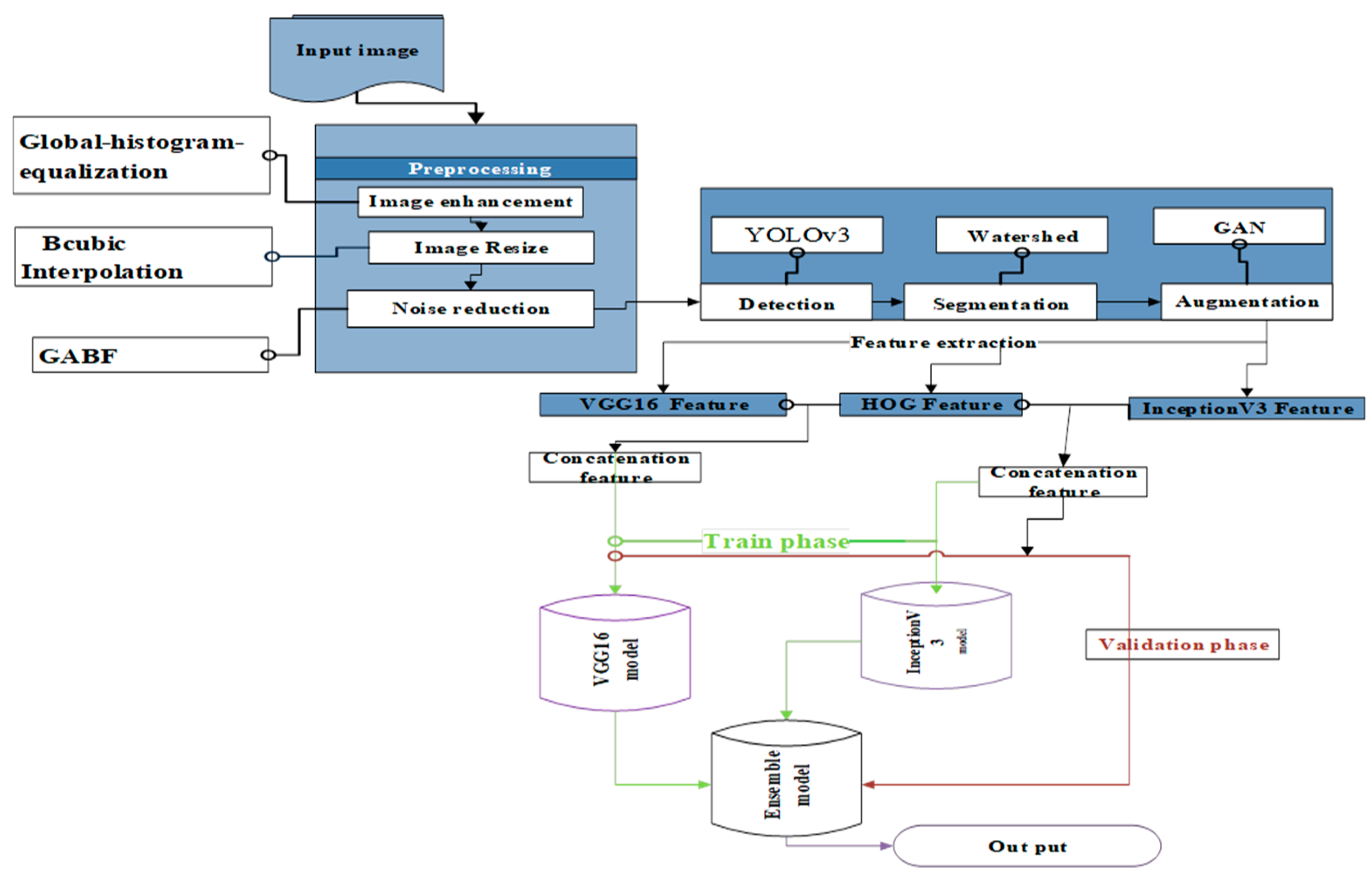
The performance of the proposed model is based on the adjustment of the independent variables. This experimental research design involves the detail of dataset preparation, preprocessing, implementation, and performance evaluation as the working architecture of
Figure 1 stated below.
The proposed architecture in
Figure 1:1 outlines a classification model design consisting of four stages. The stages are preprocessing, feature extraction, model development, and model evaluation. Each stage involves specific techniques to ensure the successful completion of the task.
3.1. Preprocessing
The collected groundnut seed image suffered from burling low insight intensity and had varying sizes with a limited imbalanced collection. These challenges required noise filtering, resizing, enhancement, and other preprocessing techniques. To choose the most effective preprocessing technique image quality evaluation metrics, such as, Mean Square Error (MSE) Structural Similarity Index (SSI), and Peak Signal Noise Ratio (PSNR) were utilized.
Image quality evaluation: In Preprocessing, the result of the image may lead to a loss of important information. Image quality evaluation (Padilla et al., 2020) can be subjective to relying on human judgment, or objective utilizing image evaluation techniques. The study (Hu et al., 2020) suggested that the subjective method is efficient in cases like multimedia images, still for other image-based applications, it may be time-consuming and result in a loss of important information (Z. Wang et al., 2004). Instead, objective methods are best suited to compare and evaluate processed images with original images or image processing algorithms. Some of these evaluation metrics include Mean Squared Error (MSE), Signal to Noise Ratio (SNR), Peak Signal-to-Noise Ratio (PSNR), Structural Content (SC), etc.
Mean squared Error (MSE): The MSE is a method used to assess the dissimilarity between two images by calculating the average of the squared differences between corresponding pixel values in a reference (original) image and a distorted (processed) image. A lower MSE value indicates a higher similarity between the distorted and the original image. MSE is a mathematical measure that does not always correlate well with human perception, especially for view and small differences between images (Hu et al., 2020). It can be expressed as follows.
where
N is the total number of pixels in the image,
I_org(x, y) is the pixel value at coordinates (x, y) in the original image, and
I_pro(x, y) is the pixel value at coordinates (x, y) in the processed image.
PSNR: It assesses and calculates the ratio between the maximum signal power and the MSE between the original and distorted images. It is typically expressed in decibels (dB) and serves as an indicator of the amount of noise or distortion present in the image. A higher PSNR value suggests that the image has a reduced amount of noise or distortion. PSNR can be calculated as
where
Function converts the ratio of the peak signal power to MSE into a logarithmic scale and multiplying by 10 scales it to decibels (
dB).
Structural Similarity Index: It assesses how similar the structures in two images are unlike conventional metrics that, only consider pixel differences on factors like luminance, contrast, and the overall structure of the image (Horé & Ziou, 2010). It captures important visual characteristics instead of just individual pixel values. When the SSIM value is higher, it signifies that the original and distorted images have a stronger resemblance in terms of their structure, implying a higher level of perceptual quality. Index similarity can be calculated as.
where:
x and
y represent the corresponding pixel values in the original and processed images.
L(x, y) is the luminance similarity, which measures the similarity in mean pixel intensities between x and y.
C(x, y) is the contrast similarity, which evaluates the similarity in variances of pixel intensities between x and y.
S(x, y) is the structure similarity, which calculates the similarity in covariance of pixel intensities between x and y. The values of
L(x, y), C(x, y), and
S(x, y) are typically calculated using the mean, variance, and covariance of pixel intensities in the corresponding patches of the images. The final SSIM value is obtained by taking the product of the three similarity components.
3.1.1. Histogram Equalization
It is an image processing technique that aims to enhance contrast and improve the visual quality of an image. Rajendran et al. (2015) illustrated that a histogram is used to segment an image into several regions by thresholding and redistributing the intensity values across the entire range. We applied Adaptive Histogram Equalization to address brightness issues in the collected image.
3.1.2. Resizing
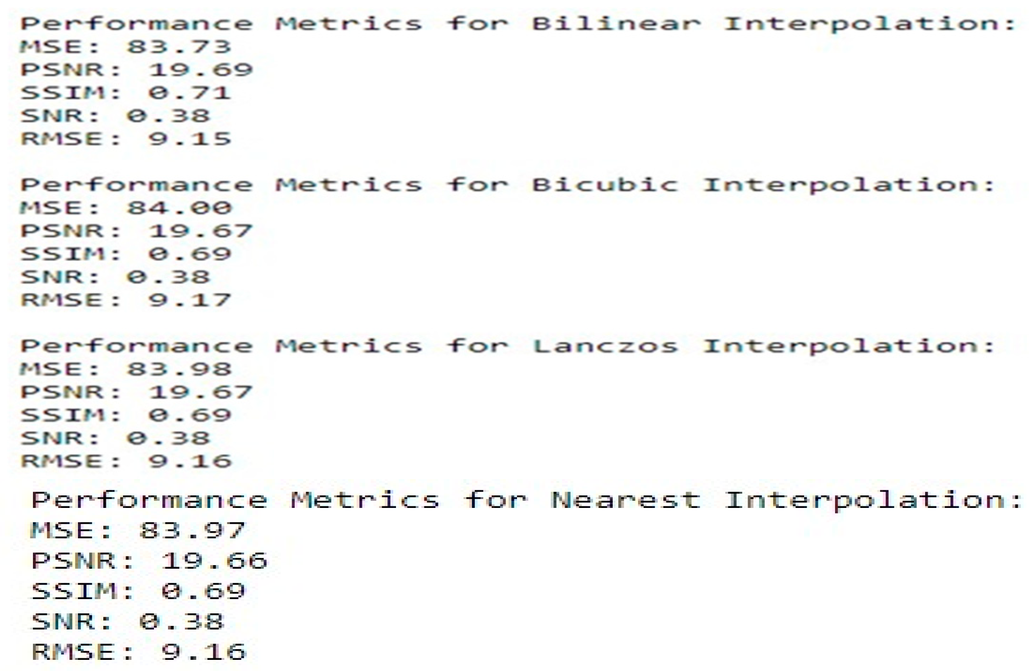
Image resizing is necessary to increase or decrease the total number of pixels. Making all experimental images uniform in dimensions helps to further preprocessing speeds in image retrieval (Gordo et al., 2017). Images are resized to 224 × 224 pixels with an aspect ratio of 2:1 by comparing resizing techniques, which include Nearest Neighbor, Bilinear Interpolation, Bicubic Interpolation, and Lanczos based on image evaluation metrics.
However, selecting the optimum resizing technique using experimental compression of objective evaluation metrics is the best strategy rather than relying on subjective evaluation in a large dataset.
Table 1 shows the values of the four resizing techniques in a single image comparison. Based on the results, the bicubic interpolation technique has been selected.
Figure 2.
Resized image quality evaluation metrics value.
Figure 2.
Resized image quality evaluation metrics value.
3.1.3. Noise Reduction
Noise removal is a technique used to eliminate unwanted detail (Motwani et al., 2004) that depreciates and destroys the original image quality. Similar to resizing techniques we have selected noise reduction techniques based on the experimental result of evaluation matrices. Based on noise reduction experimental information and evaluation results. Gaussian Adaptive Bilateral Filter (GABF) is selected from the comparison result of mean, bilateral, Gaussian, and Gaussian adaptive bilateral filtering techniques. The evaluation metrics result of PSNR and MSE in Gaussian filtering is larger than others and bilateral filtering has smaller values of MSE and PSNR from this the combination of the two has an optimum value than other techniques.
3.1.4. Segmentation
Image segmentation includes the process of digital images partitioning into meaningful multiple regions (Kunaver & Tasič, 2005) offering easy dimensional reduction. It represents some kind of information to the user in the form of color, intensity, or texture offering easier ways (Yogamangalam & Karthikeyan, 2013)for further analysis and comparison of images. Three segmentation techniques are compared through experiments on three segmentation techniques, which are watershed, threshold, and edge-based segmentation. Watershed segmentation is selected based on the characteristics of the images, which are irregular shapes and clear intensity, images with minimal overlap, and the noise is filtered by good noise reduction techniques in the previous preprocessing.
Detection
The regions of interest in the captured images are identified using YOLOv3. The detection process involves taking an input image learning the class probabilities and bounding box coordinates, and dividing the image into a grid of S x S, which predicts N bounding, boxes. The confidence level indicates the accuracy of the bounding box determining whether it contains an object (regardless of its class). Additionally, YOLOv3 predicts the classification score for each box in every image during training. The total predicted probability for all boxes is calculated as S×S×N.
GAN-Based Augmentation
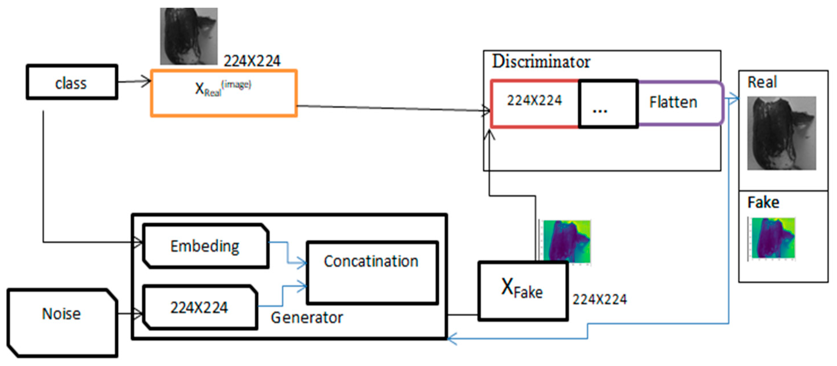
Generative Adversarial Networks (GAN)--based augmentation was applied after preprocessing the image to increase and balance the number of instances in each class. GAN is an artificial neural network, that generates a new image based on discriminator and generator networks (Frid-Adar et al., 2018) as shown below.
Figure 1.
Work of GAN-based Augmentations.
Figure 1.
Work of GAN-based Augmentations.
As shown in the Figure above, once the generator network is trained, it takes random noise as input and generates new synthetic images as training datasets. These images are fed into the discriminator network with real images from the training dataset. The discriminator then attempts to distinguish between real and synthetic images and provides feedback on the realism of the generated images. The generator network uses this feedback to enhance the quality of the synthetic images. Compared to traditional image augmentation methods such as rotation and flipping, GAN-based image augmentation can generate highly diverse and realistic images. These images can enhance the performance of deep ensemble learning models trained on limited datasets.
Table 1.
summaries of augmented images.
Table 1.
summaries of augmented images.
| Class Name |
Images in each class after augmentation |
Number of Augmented Images |
File type |
| Healthy |
1560 |
94 |
Jpg, |
| Virus defect |
1560 |
541 |
Jpg |
| Fungal defect |
1560 |
3 |
Jpg |
| physical damage |
1560 |
558 |
Jpg |
| Pest defect |
1560 |
554 |
Jpg |
| Total image |
7800 |
Ensemble Strategy
Due to the availability of vast amounts of data deep learning (Y. Yang et al., 2022) has a dominant position in various artificial intelligence applications (Livieris et al., 2021; Wyatt et al., 2022). Currently, ensemble learning techniques based on deep learning have shown significant performance improvements in learning systems. Ensemble learning (Dong & Yu, 2020; Schwenker, 2013) involves using multiple learning algorithms on a set of extracted features to gain knowledge and achieve better performance than individual weak predictive models through voting schemes. The robustness of the learning system in DEL comes from having multiple learners (neural network) (Rokibul & Nazmul, 2020; Ganaie et al., 2022) that aim to provide accurate results by combining the output of individual train neural networks instead of selecting the best one. This offers solutions to machine learning challenges by entertaining various ensemble models (Al-sahaf et al., 2019) such as averaging, stacking, boosting, etc.
Ensemble Strategies are a machine learning method that enhances a model's predictive performance by addressing the weaknesses or biases of individual models known as base learners, through the aggregation of multiple models. Effective Ensemble Strategies result in decreased overfitting, increased accuracy, and improved generalizability to unseen data. Some popular ensemble strategies include bagging, boosting, majority voting, weighted voting, averaging, and stacking. Bagging reduces variance by averaging the output of multiple models while boosting reduces bias by combining various models to enhance accuracy. Stacking involves training numerous models and using their outputs to train a final model that provides a more accurate prediction.
Majority voting is the method used to combine predictions from many individual models into a final prediction. In this method, the class labels that are most frequently predicted among the models are selected as the final prediction. It is a straightforward and powerful technique for integrating predictions from many models. It is effective in enhancing prediction accuracy across various applications.
Weighted voting: - this strategy combines predictions of several models by assigning different weights to each model according to their purposes. In this technique, each model is assigned a weighted and predicted probabilities are weighted accordingly and the final prediction is based on the weighted sum of the individual models’ predictions.
Averaging also known as voting aggregation techniques of ensemble learning is a linear combination of multiple models. The pertained model is classified,
and later an average of the results is used to make the final prediction. In the proposed, the mean approach is calculated as the following aggregated function.
where:
y is the result of the given list of models
w is the prediction of the
ith model on the
x dataset and
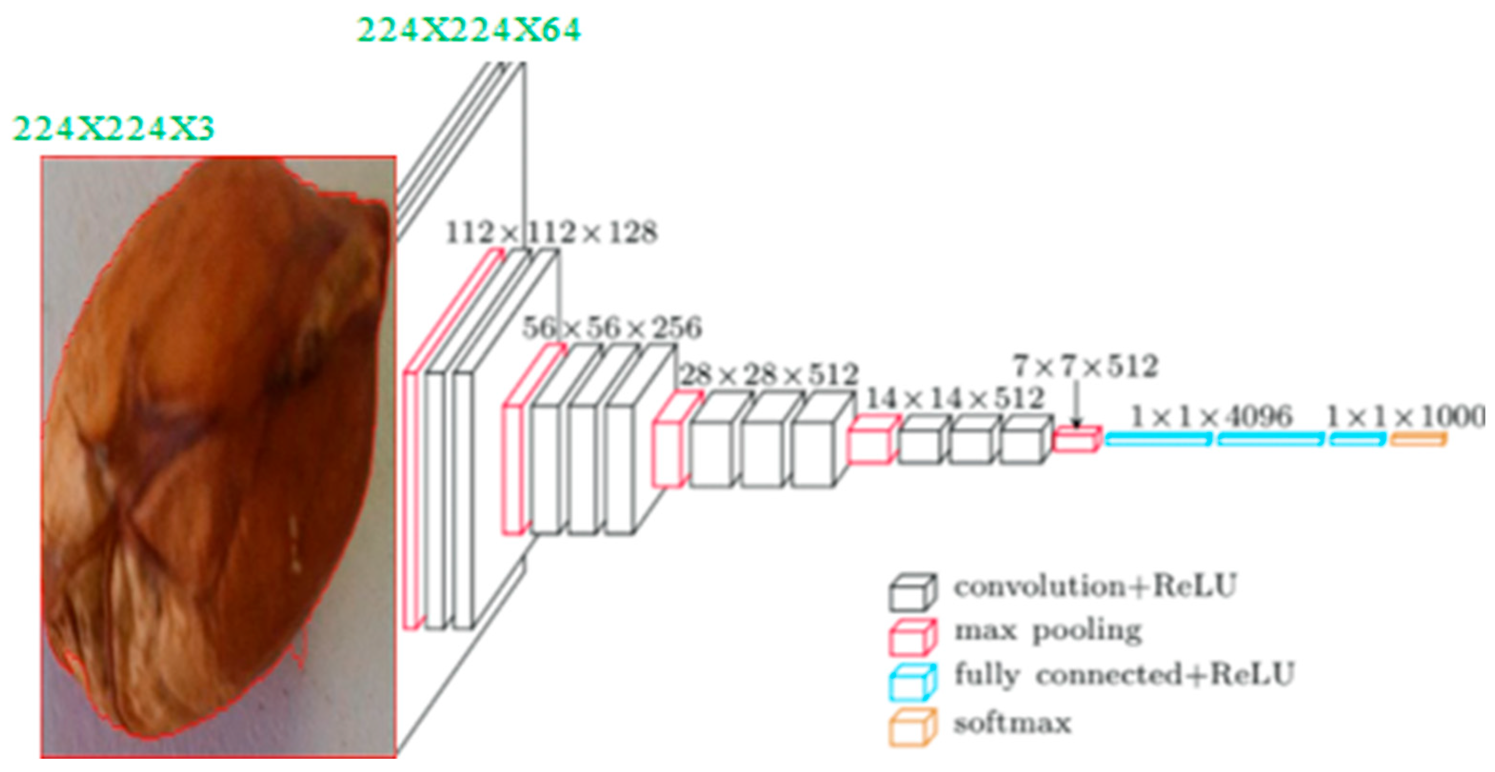
n is the number of ensemble models involved in the given problem. We use a deep ensemble learning strategy to develop averaging methods on two pre-trained models: convolutional neural network (CNN) which are VGG16, and InceptionV3 for classifications with specific ensemble strategy.
4. Experimental Result
After collecting and preparing the images; each model is individually trained with end-to-end feature extraction. After training and evaluating each model; the results show varying classification abilities. The base model uses voting aggregation to develop an ensemble model with the same data. The model is trained and evaluated using three-split ratios of 70%-15%-15%, and 80%-10%-10% for training; testing; and validation respectively with hyperparameter setup using grid search optimization. The model is trained with both GAN-based and classical augmentation techniques. However; we achieved the best result using 80%-10%-10% split ratio using GAN-based augmentation. The total number of instances used for model development is 7800 images. The validation set was calculated to be 780; while the testing set also consists of 780 image instances. The remaining 6240 image instances are allocated to the training set. Each class in the validation and testing set contained 156 images; while the training set had 1248 images for each class. The accuracy of the base and ensemble model using both augmentations is summarized in the following table
Table 1.
The result of augmented data.
Table 1.
The result of augmented data.
| Augmentation |
Base models |
Base model accuracy |
Ensemble model accuracy |
| GAN based |
VGG16 model |
94.51% |
96.25% |
| Inception V3 model |
91.31% |
| Classical |
VGG16 model |
93.56% |
94.2% |
| Inception V3 model |
90.32 |
| No augmentation |
VGG16 model |
89% |
87% |
| Inception V3 model |
83% |
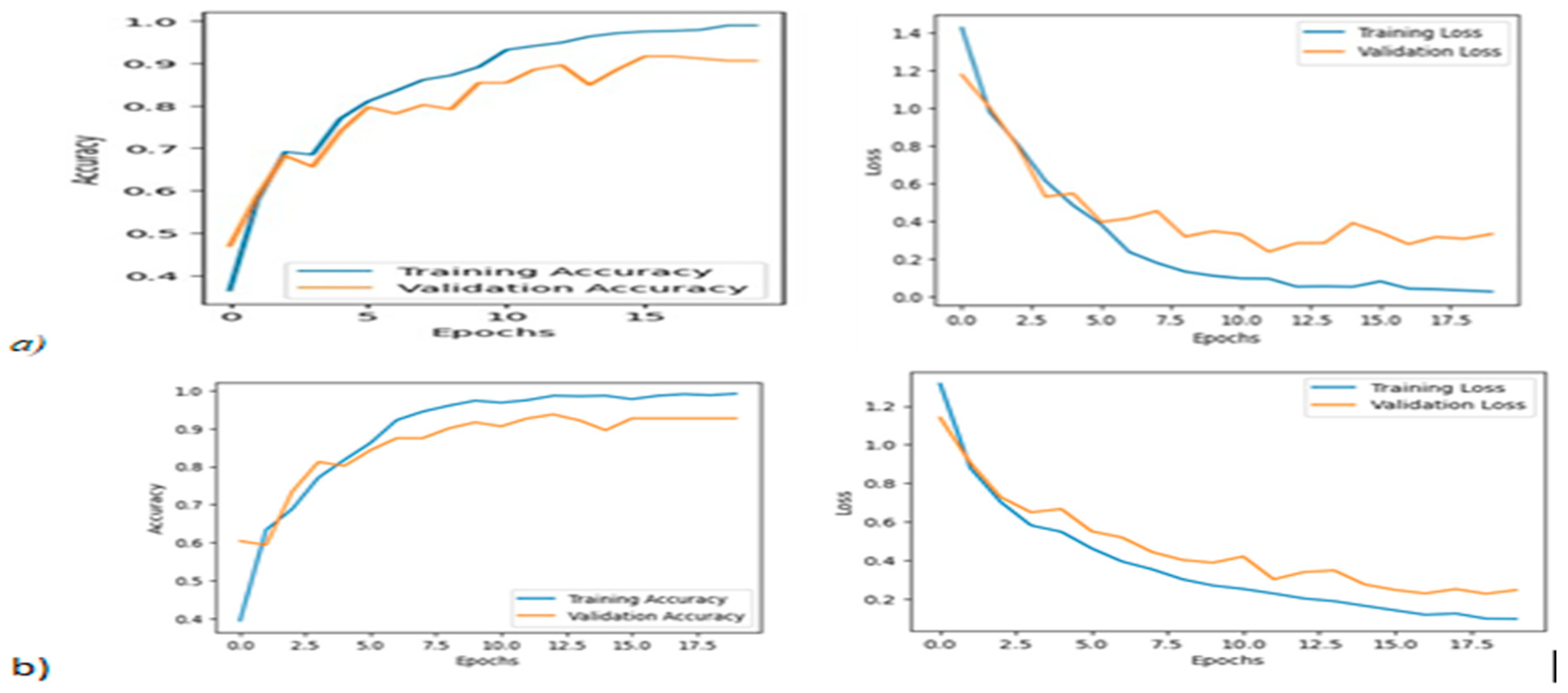
The result of the augmented data has significant differences for both the base model and ensemble model as shown in the above table. The accuracy and loss graphs of the experimental results with augmented data are represented in Figure 1.4 (a) and (b).
Figure 3.
Accuracy and loss graph of ensemble model with GAN-based and classical augmentation.
Figure 3.
Accuracy and loss graph of ensemble model with GAN-based and classical augmentation.
The model achieved 97.22%, 92.05%, and 96.25% train, validation, and test accuracy respectively. The model with GAN-based augmentation has better generalization than the classical one when we have seen the accuracy and loss graph of the model.
5. Error Analysis
The ensemble learning classification model achieved high accuracy by correctly classifying 6067 instances of training images, 718 validation images, and 751 testing images. However, misclassifications amounted to 173 images in the training dataset, 62 validation images dataset, and 29 images in the testing dataset. Most errors and misclassifications in the training, validation, and test data were due to cracked classes. The model often mistook cracked images as pest defects, classifying them as pest defective instead of pest defect images. Another error occurred with two classes, where pest-defected images were learned as cracked, and virus-defected images were considered fungal defective instead of their actual classification. To improve the model's accuracy and robustness, we suggested removing images that resemble other classes and finding additional feature extraction techniques to differentiate them. Additionally, the VGG16 pre-trained model exhibited weaker classification ability compared to InceptionV3.
6. Conclusions
In this study, Groundnut seed image defects are classified into five categories virus, fungus, pest damage, physical damage, and health using a deep ensemble model. The collected images are enhanced with Global Histogram Equalization (GHE), and noise filtered using Gaussian adaptive Bilateral Filtering (GABF) techniques. The images are resized to 224 × 224 using bicubic interpolation with an aspect ratio of 2:1. Preprocessing techniques are chosen based on image evaluation metrics. Regions of interest are detected using YOLOv3. The initial dataset of 6050 images is augmented using traditional and GAN-based methods, resulting in a total of 7800 images. The classification model is trained using features extracted from a comparison of classical techniques (GLCM & HOG) with deep-based techniques (VGG16 & InceptionV3). The experiment showed that different base learners performed differently depending on the feature concatenation with InceptionV3 performing well on deep-based and HOG features. The model evaluation without augmentation, GAN-based augmentation, and traditional augmentation achieved test accuracies of 87%, 96.25%, and 94.2%, respectively. The model’s performance is limited by the similar appearance of different defects and the weaknesses of the classification base learners. The challenges make it difficult for researchers to claim performance improvements and the effectiveness of the model.
Funding
The authors did not receive any financial support for the research, and publication of this article.
Data Availability Statement
Code Availability: The code used in this study is available from the corresponding author upon reasonable request. The data that support the findings of this study are available from the corresponding author upon reasonable request.
Acknowledgments
We would like to express our gratitude to the anonymous reviewers for their valuable comments and constructive suggestions. This research did not receive specific grants from funding agencies in the public, commercial, or not-for-profit sectors.
Conflict of Interest
The author declares no conflicts of interest for the manuscript and its forthcoming publication process.
References
- Al-sahaf, H., Bi, Y., Chen, Q., Lensen, A., Mei, Y., Sun, Y., Xue, B., & Zhang, M. (2019). A survey on evolutionary machine learning. Journal of the Royal Society of New Zealand, 49(2), 205–228. [CrossRef]
- Asibuo, J., Akromah, R., Adu-Dapaah, H., & Safo-Kantanka, O. (2008). Evaluation of nutritional quality of groundnut (Arachis Hypogaea L.) from Ghana. African Journal of Food, Agriculture, Nutrition and Development, 8(2), 133–150. [CrossRef]
- Bajia, R., Singh, S. K., Bairwa, B., & Padwal, K. G. (2017). MAJOR INSECT PESTS OF GROUNDNUT ( Arachis hypogaea L.),. August. [CrossRef]
- District, S. A. (1935). THE INHERITANCE OF CHARACTERS IN THE. 1(8).
- Dong, X., & Yu, Z. (2020). A survey on ensemble learning. 14(2), 241–258.
- Frid-Adar, M., Diamant, I., Klang, E., Amitai, M., Goldberger, J., & Greenspan, H. (2018). GAN-based synthetic medical image augmentation for increased CNN performance in liver lesion classification. Neurocomputing, 321, 321–331. [CrossRef]
- Ganaie, M. A., Hu, M., Malik, A. K., Tanveer, M., & Suganthan, P. N. (2022). Ensemble deep learning: A review. Engineering Applications of Artificial Intelligence, 115. [CrossRef]
- Gordo, A., Almazán, J., Revaud, J., & Larlus, D. (2017). End-to-End Learning of Deep Visual Representations for Image Retrieval. International Journal of Computer Vision, 124(2), 237–254. [CrossRef]
- Guchi, E. (2015). Aflatoxin Contamination in Groundnut (Arachis hypogaea L.) Caused by Aspergillus Species in Ethiopia. Journal of Applied & Environmental Microbiology, 3(1), 11–19.
- Horé, A., & Ziou, D. (2010). Image quality metrics: PSNR vs. SSIM. Proceedings - International Conference on Pattern Recognition, 2366–2369. [CrossRef]
- Hu, B., Li, L., Wu, J., & Qian, J. (2020). Subjective and objective quality assessment for image restoration: A critical survey. Signal Processing: Image Communication, 85(June), 1–50. [CrossRef]
- Huang, S., Fan, X., Sun, L., Shen, Y., & Suo, X. (2019). Research on Classification Method of Maize Seed Defect Based on Machine Vision. 2019(1).
- enber, A., Olalekan, A., Ashagrie, M., & Bitew, M. (2022). Informatics in Medicine Unlocked Development of a chickpea disease detection and classification model using deep learning. Informatics in Medicine Unlocked, 31(May), 100970. [CrossRef]
- Kunaver, M., & Tasič, J. F. (2005). Image feature extraction - An overview. EUROCON 2005 - The International Conference on Computer as a Tool, I, 183–186. [CrossRef]
- Kundu, N., & Rani, G. (n.d.). Seeds Classification and Quality Testing Using Deep Learning and YOLO v5.
- Li, Z., Gong, B., & Yang, T. (2016). Improved dropout for shallow and deep learning. Advances in Neural Information Processing Systems, Nips, 2531–2539.
- Liu, Z., Jiang, J., Li, M., Yuan, D., Nie, C., Sun, Y., & Zheng, P. (2022). Identification of Moldy Peanuts under Different Varieties and Moisture Content Using Hyperspectral Imaging and Data Augmentation Technologies. Foods, 11(8). [CrossRef]
- Livieris, I. E., Iliadis, L., & Pintelas, P. (2021). On ensemble techniques of weight-constrained neural networks. Evolving Systems, 12(1), 155–167. [CrossRef]
- Manhando, E., Zhou, Y., & Wang, F. (2021). Early Detection of Mold-Contaminated Peanuts Using Machine Learning and Deep Features Based on Optical Coherence Tomography. AgriEngineering, 3(3), 703–715. [CrossRef]
- Mohanaiah, P., Sathyanarayana, P., & Gurukumar, L. (2013). Image Texture Feature Extraction Using GLCM Approach. International Journal of Scientific & Research Publication, 3(5), 1–5.
- Motwani, M., Motwani, R., & Harris, F. (2004). Survey of image denoising techniques Survey of Image Denoising Techniques. January.
- Padilla, R., Netto, S. L., & Silva, E. A. B. (2020). A Survey on Performance Metrics for Object-Detection Algorithms. July. [CrossRef]
- Qi, H., Liang, Y., Ding, Q., & Zou, J. (2021). Automatic Identification of Peanut-Leaf Diseases Based on S tack Ensemble.
- Rajendran, S., Dorothy, R., Joany, R. M., Rathish, R. J., Santhana Prabha, S., & Rajendran, S. (2015). Image enhancement by Histogram equalization Image enhancement by Histogram equalization Image enhancement by Histogram equalization. Int. J. Nano. Corr. Sci. Engg, 2(4), 21–30.
- Rokibul, K., & Nazmul, A. (2020). A dynamic ensemble learning algorithm for neural networks. Neural Computing and Applications, 32(12), 8675–8690. [CrossRef]
- Sarvamangala, C., Gowda, M. V. C., And, & Varshney, R. K. (2011). This is the author's version of the postprint archived in the official repository of ICRISAT Identification of quantitative trait loci for protein content, oil content, and oil quality for groundnut ( Arachis hypogaea L.). 122(1), 49–59.
- Schwenker, F. (2013). Ensemble Methods: Foundations and Algorithms [Book Review]. IEEE Computational Intelligence Magazine, 8(February), 77–79. [CrossRef]
- Shasidhar, Y., Vishwakarma, M. K., Pandey, M. K., Janila, P., Variath, M. T., Manohar, S. S., Nigam, S. N., Guo, B., & Varshney, R. K. (2017). Molecular mapping of oil content and fatty acids using dense genetic maps in groundnut (Arachis hypogaea L.). Frontiers in Plant Science, 8(May), 1–14. [CrossRef]
- State, O., & State, O. (2007). Fruit Morphological Characterization among Some Varieties of. 1(2), 155–160.
- Szczypinski, P. M., Klepaczko, A., & Kociolek, M. (2017). Barley defects identification. International Symposium on Image and Signal Processing and Analysis, ISPA, September, 216–219. [CrossRef]
- Veni, N., & Manjula, J. (2022). High-performance visual geometric group deep learning architectures for MRI brain tumor classification. Journal of Supercomputing, 78(10), 12753–12764. [CrossRef]
- Wang, Y., Ding, Z., Song, J., Ge, Z., Deng, Z., Liu, Z., Wang, J., Bian, L., & Yang, C. (2023). Peanut Defect Identification Based on Multispectral Image and Deep Learning. Agronomy, 13(4). [CrossRef]
- Wang, Z., Bovik, A. C., Sheikh, H. R., & Simoncelli, E. P. (2004). Image quality assessment: From error visibility to structural similarity. IEEE Transactions on Image Processing, 13(4), 600–612. [CrossRef]
- Wyatt, M., Radford, B., Callow, N., Bennamoun, M., & Hickey, S. (2022). Using ensemble methods to improve the robustness of deep learning for image classification in marine environments. 2022(February), 1317–1328. [CrossRef]
- Yang, H., Ni, J., Gao, J., Han, Z., & Luan, T. (2021). A novel method for peanut variety identification and classification by Improved VGG16. Scientific Reports, 11(1), 1–17. [CrossRef]
- Yang, Y., Lv, H., & Chen, N. (2022). A Survey on ensemble learning under the era of deep learning.
- Yogamangalam, R., & Karthikeyan, B. (2013). Segmentation techniques comparison in image processing. International Journal of Engineering and Technology, 5(1), 307–313.
- Ziyaee, P., Ahmadi, V. F., Bazyar, P., & Cavallo, E. (2021). Comparison of different image processing methods for segregation of peanut (Arachis hypogaea L.) seeds infected by aflatoxin-producing fungi. Agronomy, 11(5). [CrossRef]
- Zou, Z., Chen, J., Wang, L., Wu, W., Yu, T., Wang, Y., Zhao, Y., Huang, P., Liu, B., Zhou, M., Lin, P., & Xu, L. (2022). Nondestructive detection of peanuts mildew based on hyperspectral image technology and machine learning algorithm. Food Science and Technology (Brazil), 42, 1–11. [CrossRef]
|
Disclaimer/Publisher’s Note: The statements, opinions and data contained in all publications are solely those of the individual author(s) and contributor(s) and not of MDPI and/or the editor(s). MDPI and/or the editor(s) disclaim responsibility for any injury to people or property resulting from any ideas, methods, instructions or products referred to in the content. |
© 2024 by the authors. Licensee MDPI, Basel, Switzerland. This article is an open access article distributed under the terms and conditions of the Creative Commons Attribution (CC BY) license (http://creativecommons.org/licenses/by/4.0/).
