Submitted:
15 August 2024
Posted:
19 August 2024
You are already at the latest version
Abstract
Keywords:
1. Introduction
2. Materials and Methods
2.1. Study Design and Participant Selection
2.2. Experimental Design and Data Collection
2.3. Data Preprocessing and Analysis
2.4. Interpretability Techniques
3. Results
| Speed (deg/s) | Muscle Group | Measurement Side | PT (Nm) | PT/BW (%) | Max Work of Repeated Actions (J) | CV (%) | Average Power (W) | Total Work (J) | Acceleration Time (s) | Deceleration Time (s) | ROM (deg) | Average Peak Torque (Nm) |
|---|---|---|---|---|---|---|---|---|---|---|---|---|
| 60 | Extensor | Healthy Side | 29.03 (43.15, 72.18) | 38.45 (64.12, 102.57) | 30.42 (51.38, 81.8) | 22.0 (10.9, 32.9) | 17.45 (21.85, 39.3) | 155.15 (190.62, 345.78) | 60.0 (60.0, 120.0) | 60.0 (120.0, 180.0) | 13.55 (99.03, 112.58) | 25.72 (33.12, 58.85) |
| 60 | Extensor | Affected Side | 21.27 (25.43, 46.7) | 32.75 (34.56, 67.31) | 27.6 (23.6, 51.2) | 42.3 (14.3, 56.6) | 11.92 (12.28, 24.2) | 106.0 (80.9, 186.9) | 100.0 (70.0, 170.0) | 60.0 (130.0, 190.0) | 25.08 (79.38, 104.45) | 14.6 (20.36, 34.95) |
| 60 | Flexor | Healthy Side | 17.48 (15.07, 32.55) | 24.94 (22.32, 47.26) | 26.9 (8.1, 35.0) | 45.9 (9.95, 55.85) | 9.88 (2.9, 12.78) | 99.8 (24.0, 123.8) | 100.0 (90.0, 190.0) | 170.0 (120.0, 290.0) | 17.3 (94.0, 111.3) | 16.5 (11.11, 27.6) |
| 60 | Flexor | Affected Side | 8.98 (8.81, 17.79) | 15.39 (12.79, 28.18) | 13.77 (0.4, 14.17) | 49.43 (22.47, 71.9) | 4.91 (0.1, 5.01) | 40.9 (1.6, 42.5) | 80.0 (110.0, 190.0) | 110.0 (140.0, 250.0) | 25.6 (83.1, 108.7) | 7.37 (5.77, 13.14) |
| 90 | Extensor | Healthy Side | 25.12 (37.92, 63.05) | 33.42 (58.2, 91.62) | 29.83 (46.3, 76.12) | 15.02 (7.48, 22.5) | 21.27 (30.68, 51.95) | 111.2 (206.4, 317.6) | 40.0 (80.0, 120.0) | 40.0 (120.0, 160.0) | 11.25 (101.9, 113.15) | 24.73 (31.95, 56.68) |
| 90 | Extensor | Affected Side | 12.84 (12.41, 25.24) | 17.16 (19.94, 37.1) | 23.45 (4.45, 27.9) | 26.65 (12.35, 39.0) | 12.35 (2.3, 14.65) | 94.5 (11.82, 106.33) | 107.5 (112.5, 220.0) | 90.0 (130.0, 220.0) | 12.12 (100.5, 112.62) | 9.54 (10.28, 19.81) |
| 90 | Flexor | Healthy Side | 5.97 (7.9, 13.88) | 8.05 (11.73, 19.78) | 9.18 (0.33, 9.5) | 35.98 (18.42, 54.4) | 6.06 (0.1, 6.16) | 28.77 (0.93, 29.7) | 50.0 (120.0, 170.0) | 70.0 (130.0, 200.0) | 28.1 (81.6, 109.7) | 5.33 (6.37, 11.7) |
| 90 | Flexor | Affected Side | 24.58 (31.9, 56.48) | 34.37 (49.52, 83.89) | 21.5 (47.4, 68.9) | 12.4 (7.1, 19.5) | 24.05 (35.12, 59.18) | 99.8 (196.8, 296.6) | 50.0 (90.0, 140.0) | 40.0 (130.0, 170.0) | 11.27 (102.2, 113.47) | 17.74 (31.21, 48.95) |
| 120 | Extensor | Healthy Side | 12.92 (25.27, 38.2) | 18.35 (37.92, 56.27) | 23.95 (23.95, 47.9) | 15.68 (6.83, 22.5) | 21.79 (19.46, 41.26) | 115.03 (92.38, 207.4) | 70.0 (130.0, 200.0) | 60.0 (150.0, 210.0) | 26.05 (83.85, 109.9) | 9.84 (22.72, 32.55) |
| 120 | Extensor | Affected Side | 10.4 (11.97, 22.38) | 14.12 (17.32, 31.45) | 19.8 (2.3, 22.1) | 24.18 (15.93, 40.1) | 14.25 (1.55, 15.8) | 80.55 (6.45, 87.0) | 67.5 (140.0, 207.5) | 77.5 (140.0, 217.5) | 11.2 (101.6, 112.8) | 9.14 (9.05, 18.19) |
| 120 | Flexor | Healthy Side | 4.59 (9.42, 14.01) | 7.04 (13.08, 20.12) | 6.83 (0.3, 7.12) | 32.3 (24.6, 56.9) | 4.7 (0.1, 4.8) | 26.83 (1.0, 27.83) | 67.5 (142.5, 210.0) | 80.0 (140.0, 220.0) | 24.5 (85.4, 109.9) | 5.2 (6.3, 11.5) |
| 120 | Flexor | Affected Side | 29.03 (43.15, 72.18) | 38.45 (64.12, 102.57) | 30.42 (51.38, 81.8) | 22.0 (10.9, 32.9) | 17.45 (21.85, 39.3) | 155.15 (190.62, 345.78) | 60.0 (60.0, 120.0) | 60.0 (120.0, 180.0) | 13.55 (99.03, 112.58) | 25.72 (33.12, 58.85) |
4. Discussion
5. Conclusion
References
- Feigin, V.L.; Stark, B.A.; Johnson, C.O.; Roth, G.A.; Bisignano, C.; Abady, G.G.; Abbasifard, M.; Abbasi-Kangevari, M.; Abd-Allah, F.; Abedi, V.; Abualhasan, A. Global, regional, and national burden of stroke and its risk factors, 1990-2019: a systematic analysis for the Global Burden of Disease Study 2019. Lancet Neurol 2021, 20, 795–820. [Google Scholar] [CrossRef] [PubMed]
- Li, S.; Francisco, G.E.; Zhou, P. Post-stroke Hemiplegic Gait: New Perspective and Insights. Front Physiol 2018, 9, 1021. [Google Scholar] [CrossRef] [PubMed]
- Frenkel-Toledo, S.; Ofir-Geva, S.; Mansano, L.; et al. Stroke Lesion Impact on Lower Limb Function. Front Hum Neurosci 2021, 15, 592975. [Google Scholar] [CrossRef] [PubMed]
- Ng, M.M.; Hill, K.D.; Batchelor, F.; et al. Factors Predicting Falls and Mobility Outcomes in Patients With Stroke Returning Home After Rehabilitation Who Are at Risk of Falling. Arch Phys Med Rehabil 2017, 98, 2433–2441. [Google Scholar] [CrossRef] [PubMed]
- Bergamini, E.; Iosa, M.; Belluscio, V.; et al. Multi-sensor assessment of dynamic balance during gait in patients with subacute stroke. J Biomech 2017, 61, 208–215. [Google Scholar] [CrossRef] [PubMed]
- Nagano, H.; Said, C.M.; James, L.; et al. Biomechanical Correlates of Falls Risk in Gait Impaired Stroke Survivors. Front Physiol 2022, 13, 833417. [Google Scholar] [CrossRef]
- Barroso, F.O.; Torricelli, D.; Molina-Rueda, F.; et al. Combining muscle synergies and biomechanical analysis to assess gait in stroke patients. J Biomech 2017, 63, 98–103. [Google Scholar] [CrossRef] [PubMed]
- Ferrarello, F.; Bianchi, V.A.; Baccini, M.; et al. Tools for observational gait analysis in patients with stroke: a systematic review. Phys Ther 2013, 93, 1673–1685. [Google Scholar] [CrossRef]
- Ishiwatari, M.; Tani, M.; Isayama, R.; et al. Prediction of gait independence using the Trunk Impairment Scale in patients with acute stroke. Ther Adv Neurol Disord 2022, 15, 17562864221140180. [Google Scholar] [CrossRef] [PubMed]
- Schwarz, A.; Al-Haj Husain, A.; Einaudi, L.; et al. Reliability and Validity of a Wearable Sensing System and Online Gait Analysis Report in Persons after Stroke. Sensors 2023, 23, 624. [Google Scholar] [CrossRef]
- Mohan, D.M.; Khandoker, A.H.; Wasti, S.A.; et al. Assessment Methods of Post-stroke Gait: A Scoping Review of Technology-Driven Approaches to Gait Characterization and Analysis. Front Neurol 2021, 12, 650024. [Google Scholar] [CrossRef] [PubMed]
- Visscher, R.M.S.; Sansgiri, S.; Freslier, M.; et al. Towards validation and standardization of automatic gait event identification algorithms for use in paediatric pathological populations. Gait Posture 2021, 86, 64–69. [Google Scholar] [CrossRef] [PubMed]
- Homes, R.; Clark, D.; Moridzadeh, S.; et al. Comparison of a Wearable Accelerometer/Gyroscopic, Portable Gait Analysis System (LEGSYS+(TM)) to the Laboratory Standard of Static Motion Capture Camera Analysis. Sensors 2023, 23, 537. [Google Scholar] [CrossRef] [PubMed]
- Yeung, L.F.; Yang, Z.; Cheng, K.C.; et al. Effects of camera viewing angles on tracking kinematic gait patterns using Azure Kinect, Kinect v2 and Orbbec Astra Pro v2. Gait Posture 2021, 87, 19–26. [Google Scholar] [CrossRef]
- Van Der Woude, D.R.; Ruyten, T.; Bartels, B. Reliability of Muscle Strength and Muscle Power Assessments Using Isokinetic Dynamometry in Neuromuscular Diseases: A Systematic Review. Phys Ther 2022, 102. [Google Scholar] [CrossRef] [PubMed]
- Mainali, S.; Darsie, M.E.; Smetana, K.S. Machine Learning in Action: Stroke Diagnosis and Outcome Prediction. Front Neurol 2021, 12, 734345. [Google Scholar] [CrossRef] [PubMed]
- Gandolfi, M.; Boscolo Galazzo, I.; Gasparin Pavan, R.; et al. eXplainable AI Allows Predicting Upper Limb Rehabilitation Outcomes in Sub-Acute Stroke Patients. IEEE J Biomed Health Inform 2023, 27, 263–273. [Google Scholar] [CrossRef] [PubMed]
- Liu, G.; Wu, J.; Dang, C.; et al. Machine Learning for Predicting Motor Improvement After Acute Subcortical Infarction Using Baseline Whole Brain Volumes. Neurorehabil Neural Repair 2022, 36, 38–48. [Google Scholar] [CrossRef] [PubMed]
- Hussain, I.; Park, S.J. Prediction of Myoelectric Biomarkers in Post-Stroke Gait. Sensors 2021, 21, 5334. [Google Scholar] [CrossRef] [PubMed]
- Kim, J.K.; Choo, Y.J.; Chang, M.C. Prediction of Motor Function in Stroke Patients Using Machine Learning Algorithm: Development of Practical Models. J Stroke Cerebrovasc Dis 2021, 30, 105856. [Google Scholar] [CrossRef]
- Wang, F.C.; Chen, S.F.; Lin, C.H.; et al. Detection and Classification of Stroke Gaits by Deep Neural Networks Employing Inertial Measurement Units. Sensors 2021, 21, 1864. [Google Scholar] [CrossRef]
- Morbidoni, C.; Cucchiarelli, A.; Agostini, V.; et al. Machine-Learning-Based Prediction of Gait Events From EMG in Cerebral Palsy Children. IEEE Trans Neural Syst Rehabil Eng 2021, 29, 819–830. [Google Scholar] [CrossRef]
- Guo, Y.; Gu, X.; Yang, G.Z. MCDCD: Multi-Source Unsupervised Domain Adaptation for Abnormal Human Gait Detection. IEEE J Biomed Health Inform 2021, 25, 4017–4028. [Google Scholar] [CrossRef]
- Veerkamp, K.; Waterval, N.F.J.; Geijtenbeek, T.; et al. Evaluating cost function criteria in predicting healthy gait. J Biomech 2021, 123, 110530. [Google Scholar] [CrossRef]
- Folstein, M.F.; Folstein, S.E.; Mchugh, P.R. “Mini-mental state”. A practical method for grading the cognitive state of patients for the clinician. J Psychiatr Res 1975, 12, 189–198. [Google Scholar] [CrossRef] [PubMed]
- Guo, Y.; Wang, W.; Wang, X. A Robust Linear Regression Feature Selection Method for Data Sets With Unknown Noise. IEEE Transactions on Knowledge and Data Engineering 2023, 35, 31–44. [Google Scholar] [CrossRef]
- Fang, X.; Yang, N. A Neural Learning Approach for a Data-Driven Nonlinear Error Correction Model. Comput Intell Neurosci 2023, 2023, 5884314. [Google Scholar] [CrossRef] [PubMed]
- Breiman, L. Random Forests. Machine Learning 2001, 45, 5–32. [Google Scholar] [CrossRef]
- Yang, W.X.; Wang, F.F.; Pan, Y.Y.; et al. Comparison of ischemic stroke diagnosis models based on machine learning. Front Neurol 2022, 13, 1014346. [Google Scholar] [CrossRef] [PubMed]
- Lundberg, S.M.; Lee, S.-I. A Unified Approach to Interpreting Model Predictions. In Proceedings of the Advances in Neural Information Processing Systems 30 (NIPS 2017) 2017. [Google Scholar]
- Nikolaou, V.; Massaro, S.; Garn, W.; et al. The cardiovascular phenotype of Chronic Obstructive Pulmonary Disease (COPD): Applying machine learning to the prediction of cardiovascular comorbidities. Respir Med 2021, 186, 106528. [Google Scholar] [CrossRef] [PubMed]
- Pickett, K.L.; Suresh, K.; Campbell, K.R.; et al. Random survival forests for dynamic predictions of a time-to-event outcome using a longitudinal biomarker. BMC Med Res Methodol 2021, 21, 216. [Google Scholar] [CrossRef] [PubMed]
- Speiser, J.L. A random forest method with feature selection for developing medical prediction models with clustered and longitudinal data. J Biomed Inform 2021, 117, 103763. [Google Scholar] [CrossRef]
- Petch, J.; Di, S.; Nelson, W. Opening the Black Box: The Promise and Limitations of Explainable Machine Learning in Cardiology. Can J Cardiol 2022, 38, 204–213. [Google Scholar] [CrossRef]
- Sijobert, B.; Azevedo, C.; Pontier, J.; et al. A Sensor-Based Multichannel FES System to Control Knee Joint and Reduce Stance Phase Asymmetry in Post-Stroke Gait. Sensors 2021, 21, 2134. [Google Scholar] [CrossRef] [PubMed]
- Geerars, M.; Minnaar-Van Der Feen, N.; Huisstede, B.M.A. Treatment of knee hyperextension in post-stroke gait. A systematic review. Gait Posture 2022, 91, 137–148. [Google Scholar] [CrossRef]
- Sibley, A.R.; Strike, S.; Moudy, S.C.; et al. The associations between asymmetries in quadriceps strength and gait in individuals with unilateral transtibial amputation. Gait Posture 2021, 90, 267–273. [Google Scholar] [CrossRef] [PubMed]
- Lyle, M.A.; Jensen, J.C.; Hunnicutt, J.L.; et al. Identification of strength and spatiotemporal gait parameters associated with knee loading during gait in persons after anterior cruciate ligament reconstruction. J Athl Train 2021, 2021. [Google Scholar]
- Lyle, M.A.; Jensen, J.C.; Hunnicutt, J.L.; et al. Associations of Strength and Spatiotemporal Gait Variables With Knee Loading During Gait After Anterior Cruciate Ligament Reconstruction. J Athl Train 2022, 57, 158–164. [Google Scholar] [CrossRef]
- Tanaka, K.; Anan, M.; Tsubouchi, Y.; et al. Gait analysis of a patient who underwent complete resection of the patella and quadriceps femoris for soft tissue sarcoma. Eur J Phys Rehabil Med 2021, 57, 298–302. [Google Scholar] [CrossRef]
- Neuman, R.M.; Shearin, S.M.; Mccain, K.J.; et al. Biomechanical analysis of an unpowered hip flexion orthosis on individuals with and without multiple sclerosis. J Neuroeng Rehabil 2021, 18, 104. [Google Scholar] [CrossRef] [PubMed]
- Wang, K.; Tian, J.; Zheng, C.; et al. Interpretable prediction of 3-year all-cause mortality in patients with heart failure caused by coronary heart disease based on machine learning and SHAP. Comput Biol Med 2021, 137, 104813. [Google Scholar] [CrossRef] [PubMed]
- Khadem, H.; Nemat, H.; Elliott, J.; et al. Interpretable Machine Learning for Inpatient COVID-19 Mortality Risk Assessments: Diabetes Mellitus Exclusive Interplay. Sensors 2022, 22, 8757. [Google Scholar] [CrossRef] [PubMed]
- Smole, T.; Zunkovic, B.; Piculin, M.; et al. A machine learning-based risk stratification model for ventricular tachycardia and heart failure in hypertrophic cardiomyopathy. Comput Biol Med 2021, 135, 104648. [Google Scholar] [CrossRef] [PubMed]
- Jiang, Z.; Han, Y.; Xu, L.; et al. The NEAT Equating Via Chaining Random Forests in the Context of Small Sample Sizes: A Machine-Learning Method. Educ Psychol Meas 2023, 83, 984–1006. [Google Scholar] [CrossRef] [PubMed]
- Zhang, C.; Bengio, S.; Hardt, M.; et al. Understanding deep learning (still) requires rethinking generalization. Commun ACM 2021, 64, 107–115. [Google Scholar] [CrossRef]
- Dudek, G. A Comprehensive Study of Random Forest for Short-Term Load Forecasting. Energies 2022, 15, 7547. [Google Scholar] [CrossRef]
- Deng, F.; Huang, J.; Yuan, X.; et al. Performance and efficiency of machine learning algorithms for analyzing rectangular biomedical data. Lab Invest 2021, 101, 430–441. [Google Scholar] [CrossRef]
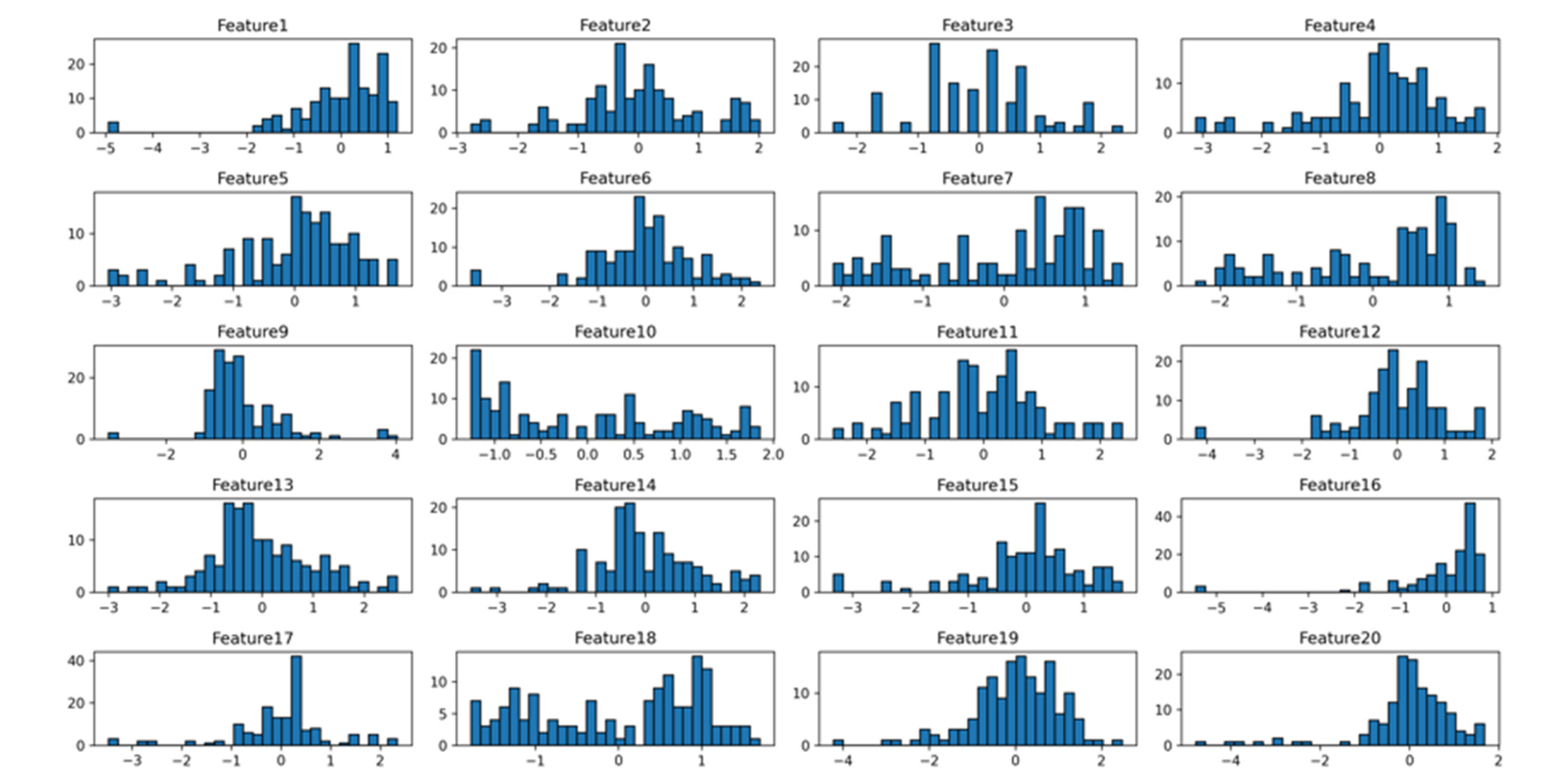
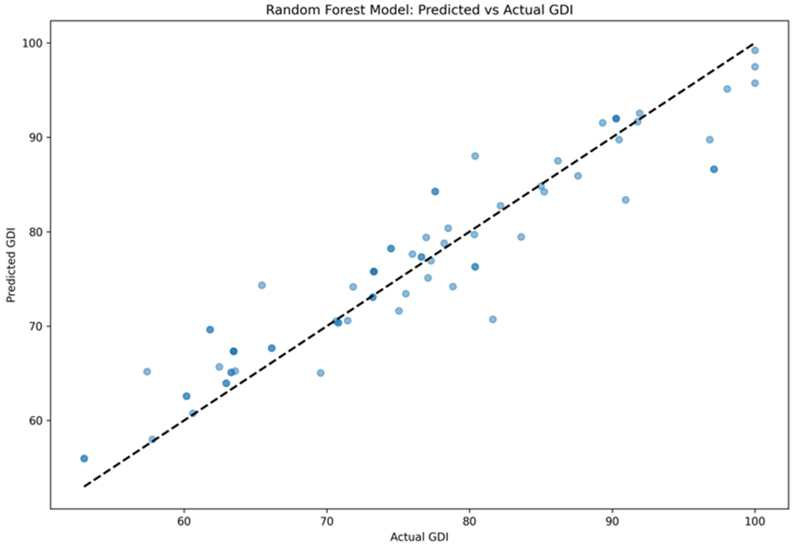
| Method | Parameter | Setting Value |
|---|---|---|
| RFE | Model Type | Linear Regression (L1 Regularization) |
| Number of Selected Features | 20 | |
| Number of Iterations | 10 | |
| Step Size | 2 | |
| Lasso Regression | α (Regularization Strength) | 0.01 |
| Max Iterations | 2000 | |
| Random State | 21 | |
| BP Neural Network | Hidden Layers | 4 layers, 12 neurons each |
| Activation Function | ReLU | |
| Optimizer | Adam | |
| Learning Rate | 0.0005 | |
| Batch Size | 64 | |
| Training Epochs | 300 | |
| RF | Number of Trees | 150 |
| Max Depth | 20 | |
| Min Samples Split | 5 | |
| Random State | 21 | |
| SVR | Kernel Function | RBF |
| Regularization Parameter C | 0.5 | |
| ε | 0.05 | |
| Max Iterations | 2000 |
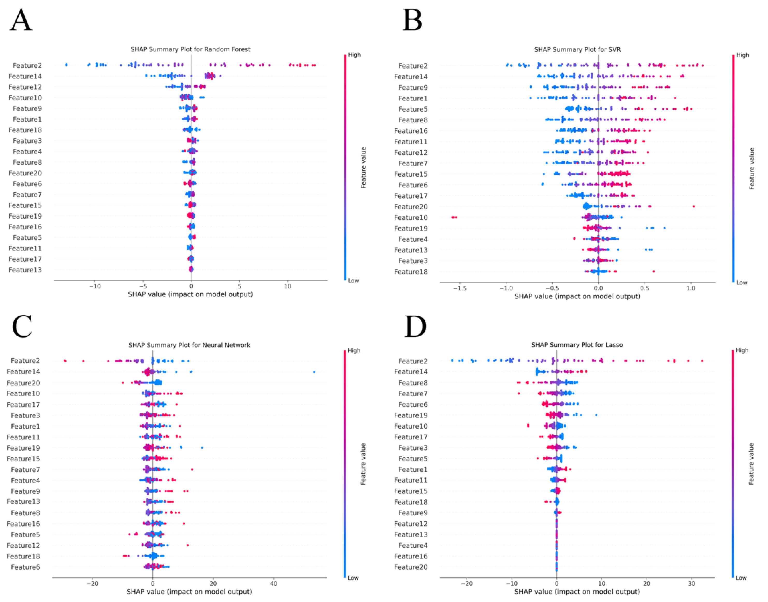
| New Feature Name | Original Feature Name |
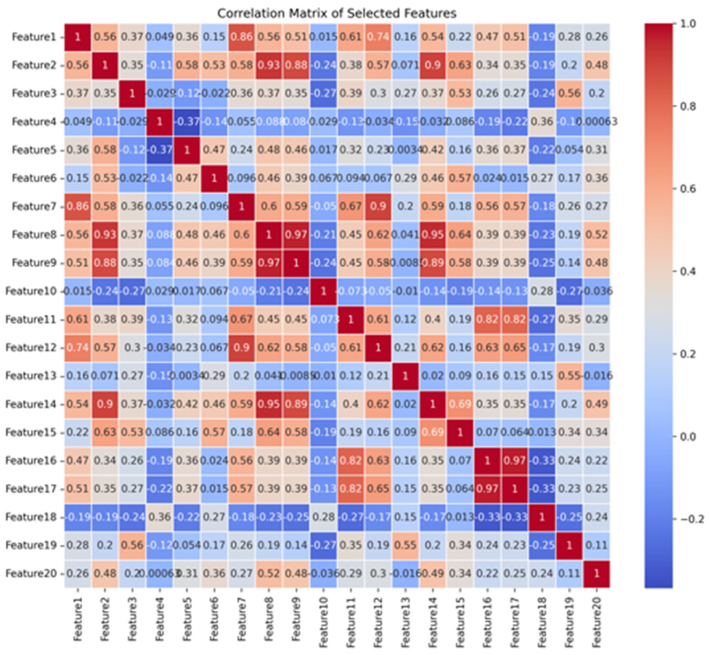
| Feature1 | 60deg_ext_healthy_max_work |
| Feature2 | 60deg_ext_affected_max_work |
| Feature3 | 60deg_flex_healthy_rom |
| Feature4 | 60deg_flex_affected_cv |
| Feature5 | 60deg_flex_affected_total_work |
| Feature6 | 60deg_flex_affected_rom |
| Feature7 | 90deg_ext_healthy_max_work |
| Feature8 | 90deg_ext_affected_max_work |
| Feature9 | 90deg_ext_affected_total_work |
| Feature10 | 90deg_ext_affected_dec_time |
| Feature11 | 90deg_flex_healthy_max_work |
| Feature12 | 120deg_ext_healthy_total_work |
| Feature13 | 120deg_ext_healthy_rom |
| Feature14 | 120deg_ext_affected_max_work |
| Feature15 | 120deg_ext_affected_rom |
| Feature16 | 120deg_flex_healthy_max_work |
| Feature17 | 120deg_flex_healthy_total_work |
| Feature18 | 120deg_flex_healthy_acc_time |
| Feature19 | 120deg_flex_healthy_rom |
| Feature20 | 120deg_flex_affected_total_work |
| Model | MSE | R2 | MAE |
| Lasso | 22.29 ± 3.28 | 0.85 ± 0.18 | 3.71 ± 0.96 |
| Random Forest | 16.18 ± 1.92 | 0.89 ± 0.06 | 2.99 ± 0.69 |
| SVR | 31.58 ± 5.48 | 0.82 ± 0.13 | 7.68 ± 1.70 |
| BP Neural Network | 50.38 ± 9.12 | 0.79 ± 0.21 | 9.59 ± 1.99 |
Disclaimer/Publisher’s Note: The statements, opinions and data contained in all publications are solely those of the individual author(s) and contributor(s) and not of MDPI and/or the editor(s). MDPI and/or the editor(s) disclaim responsibility for any injury to people or property resulting from any ideas, methods, instructions or products referred to in the content. |
© 2024 by the authors. Licensee MDPI, Basel, Switzerland. This article is an open access article distributed under the terms and conditions of the Creative Commons Attribution (CC BY) license (http://creativecommons.org/licenses/by/4.0/).


