3.1. Theoretical aspects
The distribution law establishes the correspondence between the random values,
xi, and the respective probabilities,
pi using an analytical relationship, as follows:
P(X = xi) = P(xi) = pi called probability function or distribution function,
F(x), which it can be empirical or theoretical. If the probability of the phenomenon/process
(X = xi), i.e.
P(X = xi) is obtained through experience based on statistical observation data, then the statistical probability is a relative frequency, and the distribution is empirical. The failure function,
F(x) is the most representative characteristic of a random variable and defines the probability of the phenomenon/process, that the variable value,
X be less than the value of a given
x:
If the random variables,
X follow a continuous statistical distribution, the function,
F(x) has the form:
where,
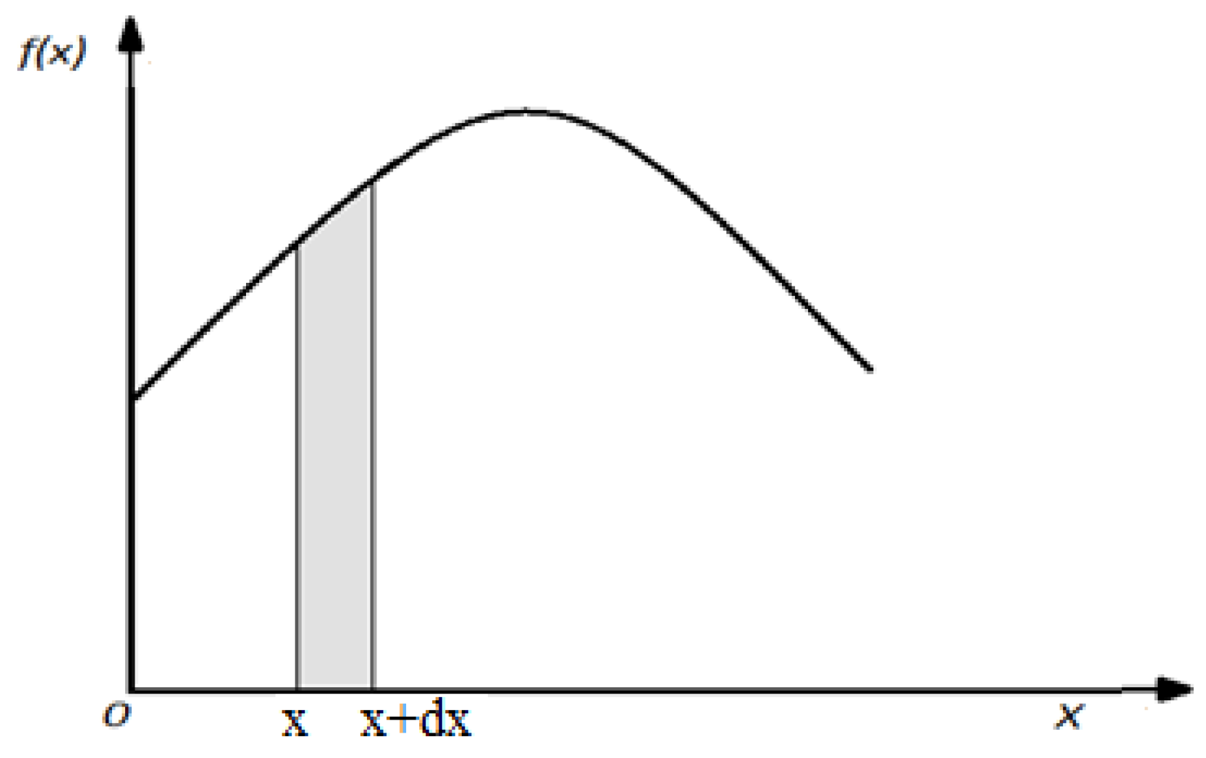
f(x) - is the frequency function (probability distribution density), which is the derivative of the function,
F(x), and
R(x) – is the reliability function. The plot of the function,
f(x) is illustrated in
Figure 3.
The value of the quantity,
f(x)dx represents the probability that the variable,
x belongs to the elementary interval,
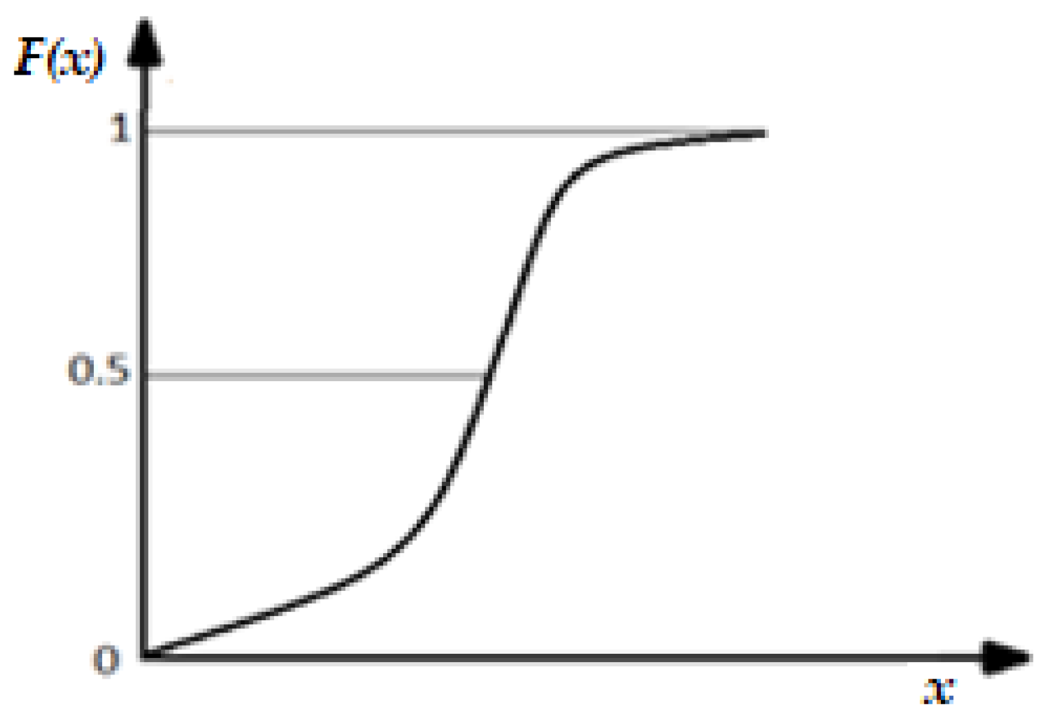
dx. The function plot, F(x) from
Figure 4 looks that:
that is, the area bounded by the function curve,
f(x), and the abscissa axis is equal to unity.
When studying a quality characteristic, the experimenter has at his disposal observational data obtained by measurements of durability. This durability is a random variable. Even if its distribution is not known, certain indicators, and certain measures [
7] of the trend of the considered variable are necessary.
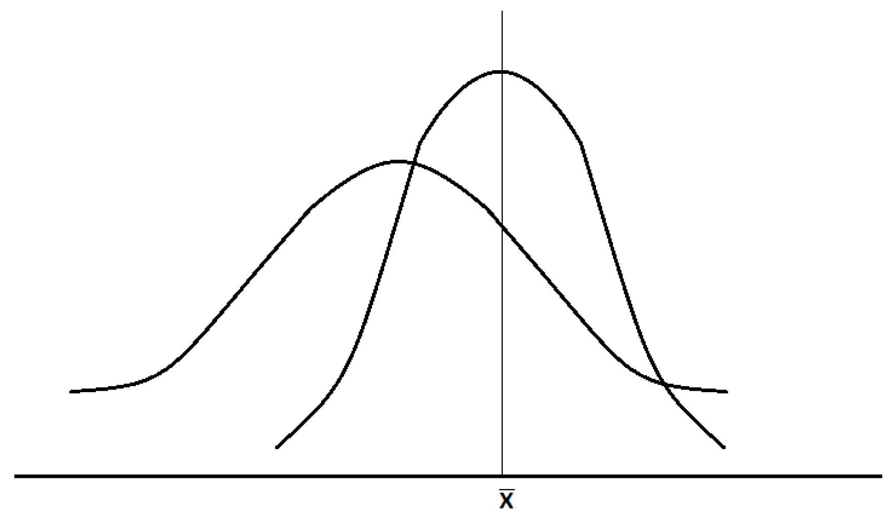
An experimental distribution (obtained through observations), respectively empirical, shows that for any characteristic of the population, a variation tendency with two aspects is generally observed: localization around a certain value (position), respectively variation (scattering),
Figure 5.
They are phenomena located around the same values, but they present different scatters (see
Figure 5). It is noted that the distribution can be symmetrical or asymmetrical about the location area. There are several statistical indicators with which a quantitative analysis can be performed to compare trends in location and variation (dispersion), namely:
a)
Location indicators - indicate the value where the actual data of the phenomenon/process tends to cluster. The main trend location indicator is the average [
12] (arithmetic average, being the most important),
M(X) and
b)
Variation indicators - those indicators that represent the deviation of the values,
x from their arithmetic mean and include:
-
dispersion, D(X) or with σ
2 (σ =
) – represents the square mean deviation), if it is defined about the mean value,
and mathematically the relation is given:
The average squared deviation, σ calculated is a "guarantee" of the accuracy of the determinations and can only be calculated if there are at least three values [
8]. On the other hand, the value of the mean square deviation, σ allows conclusions to be drawn only if it comes from at least 30 values and, at the same time, the calculation is made only if the distribution is normal (Gaussian) or almost Gaussian.
-
quartile of the random variable,
Xα defined as the equation root:
and is another reliability indicator, and α is defined as percentile
This indicator expresses the time at which a system or its component works with a certain probability (1 – F(x)).
The first collected data on the values of the investigated characteristic are presented as a disordered table. By ordering the collected (experimental) data, the statistical/statistical string (series) is obtained. Sorting is usually done in ascending order.
Data grouping is done on grouping intervals, the size of which is generally taken to be equal, except for extreme intervals, when different values can be used. The grouping intervals can be set as a number with the relation [
7,
13, and
14]:
where,
Z is the record data total number.
The size (amplitude) of the interval (class) is:
where,
xmax and
xmin are the maximum and minimum values of the data string [
7,
8,
14,
15].
During the execution of tests and the collection of experimental data, values appear that are substantially different in size from the other values, they are much smaller or much larger than the rest of the respective statistical series. Because of this, it is natural to suspect these data as "outliers", i.e. they are not from the statistical/statistical string/series. These are due to specific random influencing factors, measurement errors due to devices, operators, data recording mistakes, or data coming from a phenomenon/process other than the one under study. Until now, no absolute criterion has been established for the instant recognition of the presence of outliers [
8], which differ clearly (glaringly, visibly) from the other values of the statistical series.
There is a rich palette of tests (statistical criteria) to identify the presence of outliers. But to minimize "outlier" data/values, it is necessary to reach the state of stability (it does not mean, however, that all the causes generating outliers are canceled). This is possible, when the two parameters of the selection are known: the mean, , and the dispersion, D(X), respectively the mean square deviation, σ of the data. Because statistical tests are used when the values come from a normal (Gaussian) distribution, some of the main statistical parameters are checked.
For the analysis of a parameter, it can be estimated pointwise (as an isolated value) or with a confidence interval or significance threshold, if an interval is established that includes a probability,
P, the true value of the estimated parameter (the degree of precision of the estimate or the probability of the estimate). Therefore, the probability value,
P, implies a certain interval,
(x1, x2), according to the relationship:
and to which the respective parameter belongs.
It is mentioned that there is a "risk" or the probability that the true value will fall outside the considered confidence interval.
Depending on how the risk is placed on the confidence interval, it can be:
- confidence interval with bilateral risk (symmetric or asymmetric - the risk is placed with equal values, (α/2) on either side of the extreme values of the interval, Figure 6).
Analyzing Figures 10 and 11 it can be seen that R(t) is monotonically decreasing, instead, F(t) is increasing. These functions take values in the range [0,1] because when t → ∞, R(t) = 0, F(t) = 1, and when t → 0, R(0) = 1, F(0) = 0 and f(t) verifies the relationship .
The dental burs' reliability can also be specified with the help of the numerical values of the indicators attached to the operating time, t (variable), until the first failure. These indicators (presented above) are: M(t), D(t), σ, and tα, etc.
The values, M(t) of the operation time without failure are determined with relation (4)and presented in Table 2. By integration of the function, M(t), was obtained t = 20,433 hours, in the working conditions at the rotation speed of 7000 rpm.
The system (the dental bur active part) is without reconditioning, then M(t) represents the average time without system failure, until the first failure. M(t) of the system, i.e. the average value of t, can be expressed either by function R(t) or function f(t) (see relation (4)).
The variation of the random variable, t, or the distribution variation, D2(t) is defined by relation (5) and is obtained D2(t) = 2.562 hours, and the mean square deviation, σ, of t, is the indicator that can often be used instead of the D2(t) and results from 1.600 hours.
D2(t) and σ show the degree of uniformity of system/product performance (here, dental burs of the same type) from the point of view of reliability, by their values. If the technological process of manufacturing the system/product is well established, then the D2(t) and σ values are relatively small and show us the degree of uniformity of the set of tested dental burs, in the present case.
The last important reliability indicator considered is the operating time quartile,
tα, defined as the root of the equation:
what results from equation/relation (6) and
α with values from 0.01...0.99, is defined as a percentile.
At a rotation speed of 7000 rpm and α = 0.99 was obtained tα = 21,502 hours. In the reliability theory, the value his tα is interpreted as a guaranteed time, i.e. the period when the defective elements proportion in a certain system/group does not exceed the value, α pre-set [
4]. The value of
tα = 21,502 hours is very close to
t2 = 21,573 hours, calculated analytically, which justifies the correlation between the theoretical and experimental results.
As stated above, the first data collected regarding the values of the investigated parameter (the lost mass by the dental bur active part) is presented as a disordered mass, and by ordering (ascending) of the experimental data, the statistical series is obtained.
The grouping of the data is done on grouping intervals, whose number, n calculated with relation (7) is n = 5 (must be an integer and it was considered Z = 16 tested dental burs) and whose size is generally taken to be equal, except for the extreme intervals, when can use different values. The size (amplitude) of the interval is determined based on relation (8) and is A = (1.4 – 0.5)/5 = 0.18.
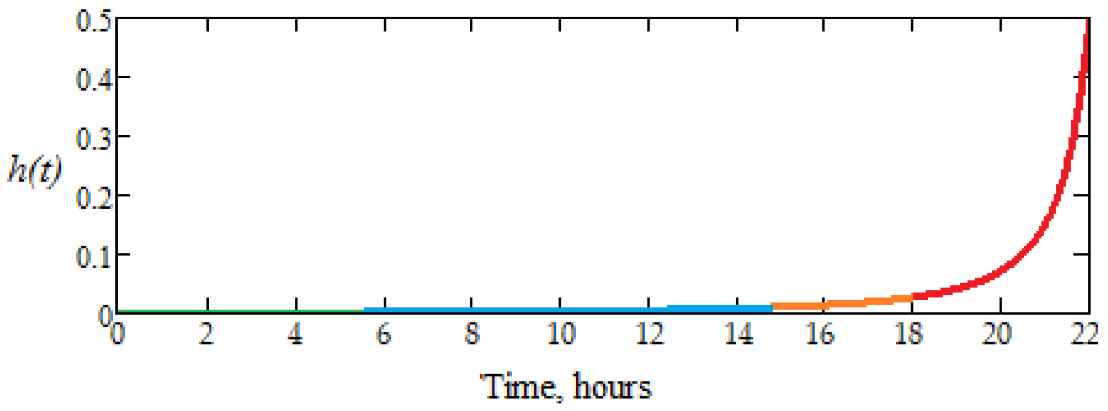
Another important role in the reliability theory has it too also the function,
h(t) = f(t)/R(t), R(t) ≠ 0 that measures the intensity (rate) of failure (the instantaneous risk of failure), or the hazard of a system/component product, defined as the failure rate limit in the interval [t , t+Δt], Δt > 0 very small [
4], whose variation is presented in
Figure 12, was used.
It can be seen that the failure risk rate is around 10%, for 20 hours and increases approximately exponentially in the 21st hour of operation. This means that the dental bur active part is taken out of operation after 20 operation hours and is normal that it be replaced.
The evolution of function h(t) shows that there is no failure risk, in the range t Є (0, 14) hours, the variation being linear, with a very small slope. In the range t Є (14, 18), the wear phenomenon becomes visible because h(t) has a variation after a fast-growing curve, and the failure risk increases. Then, in the range t Є (18, 21) hours, the failure risk becomes inevitable, when the plot of h(t) increases, after an exponential curve, suddenly.
Therefore, it is confirmed the experimental results correlate, with the analytical ones for the researched dental burs, i.e. can work without major risk of failure for up to 18 hours. At the same time, this proves the closeness between the hours determined analytically based on the experimental results to those of operation without a major failure.
On the other hand, when measuring by weighing of mass lost through wear by the dental burs active part and presented in Table 2 obtained different random values, each value having several repetitions, so a frequency of its own. These values are located in an interval with two limit values (lower and upper).
The values distribution between the limit two ones of the range can vary (with their frequency) after a distribution law. It is mentioned that the variation range of a property/characteristic/parameter reflects the quality level of a product of industrial manufacturing.
The lost mass values through effective wear (random variable) are distributed after the normal (Gaussian) distribution law because factors that determine their dispersion through wear are of the same order, accidental and independent, in large numbers and must be less than a given value what corresponds to a probability, p, i.e. of reliability, R(t)).
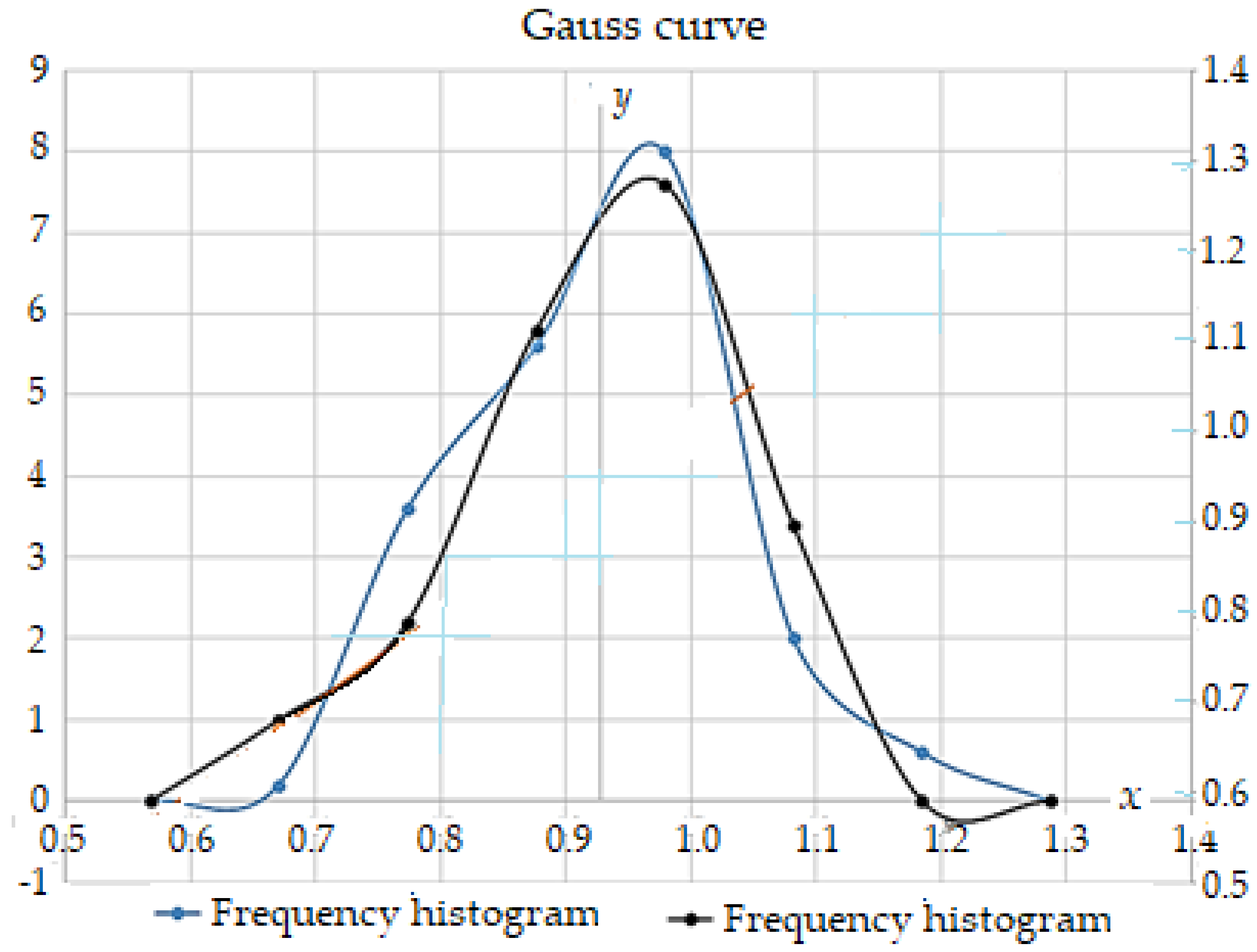
The normal distribution or Gaussian, represents the frequency function or probability distribution density, f(x), which is closest to a normal distribution function, of the shape:
whose variation over time is shown in
Figure 13.
It is observed on the probability density function curves two inflection points, of abscissas 0.88 and 1.08, where the area bordered by these abscissas and curves represents about 58.33% of the entire surface.
This proves that the values of mass lost by wear of dental burs active part are the most distributed.
The curves present a maximum of approximately, y = 5.03 at x = 0.95 (blue curve) and y = 4.98 for the same x = 0.95 (curve black), the reliability obtained being approximately 97.42% of the entire area (i.e., limited by the curves and the abscissa axis, in the range (0.67, 1.18) - confidence range), so, a reliability excellent, and the intervals (-∞, 0.67) and (1.18, +∞) can be practically neglected.
Thus, the scattering/confidence range is (0.67, 1.18), with limit deviations of ± 0.25 compared to the values distribution center (cluster), and the critical range is (-∞, 0.67) U (1.18, +∞). Therefore, the lost mass values through wear have a Gaussian (normal) distribution, and the function, f(x) is a normal distribution function or the probability distribution density (the blue and black curves from
Figure 13).
