Preprint
Article

Research on Evolutionary Algorithm for Soybean Seedling and Weed Identification Driven by Computational Complexity

Altmetrics

Downloads

66

Views

24

Comments

0

Submitted:

19 August 2024

Posted:

27 August 2024

You are already at the latest version

Alerts
Abstract
To achieve real-time identification of soybean seedlings and weeds in soybean seedling fields on agricultural intelligent terminal devices, this article constructs a real-time evolutionary identification system ESWIM driven by computational complexity under few-shot training. Firstly, based on the identification task, high-quality image samples are collected and annotated. By analyzing the terrain, the weather during the growth period, image acquisition methods, and the status of equipment fieldwork, we obtained a suitable enhancement algorithm. This algorithm not only effectively simulates the diversity of actual images, but also solves the problem of significant imbalance in the number of targets. Then, using the computational complexity driven approach and YOLOv5n as the foundation model, a soybean seedling and weed recognition model SWIM is constructed. The model's computational space and time complexity are reduced by 45.19% and 42.86%, respectively, while mAP (0.5) increased by 0.1%. Finally, by utilizing human-computer interaction to enable real-time and effective evolution of the dataset, an evolutionary strategy is designed to rapidly iterate and update model parameters, resulting in the development of the evolutionary system ESWIM. Laboratory experiments have shown that the ESWIM system can quickly adjust the recognition system during device operation to achieve target identification tasks in different environments.
Keywords: 
Subject: Biology and Life Sciences  -   Agricultural Science and Agronomy

1. Introduction

Soybean is an important oil crop variety in China, playing a crucial role in the food structure of the Chinese population [1]. In recent years, due to the complex and variable natural growth environment, soybean yield has been declining year by year. Grass damage is one of the important reasons for the decrease in soybean yield. Especially in the soybean seedling stage, its grass yield accounts for 60% of the total grass yield. These weeds compete with soybean seedlings for sunlight, water, and living space, hindering soybean growth [2]. At the same time, weeds during the soybean seedling stage will not be completely blocked by soybean seedlings, making it the best time for weed control in soybean fields. Traditional manual weed control methods are time-consuming and inefficient, and improper use of herbicides can directly pollute the soil and ecological environment. With the promotion of smart agriculture [3], using intelligent terminals to achieve soybean growth management is an important application scenario. Therefore, it is particularly important to study and implement a low computational complexity and efficient soybean seedling and weed recognition model during the seedling stage. According to the information provided by researchers from the local Academy of Agricultural Sciences, the model's weed recognition rate needs to reach 80% before it can be applied to actual devices. However, the leaf patterns and shapes of soybean seedlings in natural growth environments are similar to those of some weed species, and associated weeds grow cross with soybean seedlings, causing severe obstruction. Therefore, identifying soybean seedlings and their associated weeds has become a difficult task.
Previous weed detection methods, which primarily rely on image processing techniques, identify targets based on their color, spectrum, texture features, and shape parameters. These approaches include hyperspectral imaging and supervised learning algorithms. Liu et al. [4] conducted a weed identification study on a carrot seedling field using hyperspectral imaging techniques. However, this approach requires expensive equipment and complex operation processes, limiting its widespread application. Nahina et al. [5] conducted a weed detection analysis on a pepper field using supervised learning algorithms like Random Forest and Support Vector Machine. Although these algorithms offer simplicity and higher accuracy compared to hyperspectral imaging, they are sensitive to environmental factors and may not perform well in the complex natural environment of soybean seedling fields. With the rise of deep learning, convolutional neural networks (CNNs) have demonstrated remarkable performance in plant classification, particularly in weed detection. Tao et al. [6] combined the classical convolutional network VGG16 [7] and the fully convolutional network [8] to classify plant images, achieving an accuracy of 97.23%. Wen De Sheng et al. [9] used a deep convolutional network and a color migration method to identify weeds under natural light conditions, achieving a recognition rate of 90.01%. He et al. [10] proposed an improved EDS-YOLOv8 algorithm for weed recognition in corn fields, improving the mAP by 6.4% compared to the original Yolov8 [11]. Zhang et al. [12] used an improved Faster R-CNN [13] algorithm to effectively recognize soybean seedlings and three types of weeds in complex backgrounds, achieving an average recognition accuracy of 99.16%. This model demonstrated superior performance compared to the SSD [14] and Yolov4 [15] algorithms. Although the aforementioned model has achieved favorable recognition results, its high complexity makes it challenging to deploy on intelligent agricultural terminal devices with limited memory and computational resources.
Currently, weed control equipment relies on resource-intensive target detection models, which often fail to meet the demands for real-time, accurate, and fast identification. Therefore, efficient and lightweight methods to detect and identify soybean seedlings and weeds are essential for achieving effective weed control. Numerous studies have shown that YOLOv5 can be used effectively in multiple applications [16,17]. Several studies have explored lightweight approaches to improve the performance of target detection models. Wang et al. [18] improved the YOLOv5 model for corn and weed detection, achieving a 3.2% increase in average recognition accuracy and reducing the model file size to 14.4MB. Deng et al. [19] designed a lightweight network architecture, AlexNet-FCN, to detect rice and weeds. It obtained 80.9% accuracy with an inference speed of 4.5 fps on a Jetson TX2. Wang et al. [20] experimented with an improved lightweight sum-product network for soybean seedlings, grass weeds, broadleaf weeds, and soils detection, achieving a 99.5% average recognition accuracy with 33% fewer parameters than the traditional sum-product network [21] and a memory reduction of 549 MB. Ren et al. [22] proposed a refined YOLOv8 algorithm for cotton field weed detection, achieving 4.7% and 5.0% improvements in average recognition accuracy on two public datasets and reducing the model parameters to 6.62 MB. Ji et al. used the lightweight network PP-LCNet [23] as a feature extraction network combined with the Ghost convolution module and the NAM [24] attention module to improve the YOLOv5 network using corn seedlings and weeds as the detection targets. The lightweight network had an average accuracy of 97.8% and the model was reduced to 6.23MB, reducing complexity while maintaining recognition accuracy. Razfar et al. [25] explored an edge-based vision system for soybean garden weed detection, demonstrating that a 5-layer CNN architecture achieved the best results with a maximum accuracy of 97.7% using ResNet50 [26], MobileNet [27] and three custom CNNs [28]. The accuracy of the aforementioned model fluctuates under the premise of lightweight, but it does not identify specific weed species. Therefore, in order to better manage farmland intelligently and collect diverse plant information, we need to identify plants accurately. Therefore, in this article, we collectively refer to it as identification, which includes the detection and identification of soybean seedlings and weeds.
Despite the remarkable advancements in deep learning for weed detection, deploying these models on mobile terminals and edge devices for the efficient management of expansive agricultural fields presents several challenges. Firstly, storage space limitations: Agricultural terminal devices often have limited storage space. Therefore, in order to effectively reduce memory requirements, it is necessary to deploy low-complexity models. This is equally important for weed detection in the cloud, as low complexity can reduce the size of the model, thereby reducing storage requirements. Secondly, in the complex natural environments encountered in agriculture, real-time performance is indispensable for the accurate identification of soybean seedlings and diverse weeds. Lightweight models, by their nature, exhibit faster inference speed and quicker response rates, which align with the demands for real-time performance. Thirdly, the identification of specific weed species: the model can identify specific weed species with low computational complexity, which is crucial for meeting the actual agricultural needs. This requires ensuring the accuracy of weed identification while maintaining the efficiency of the model. Finally, there are various complex landscapes and weather conditions in natural environments, so a model with strong generalization ability can more stably identify soybean seedlings and weeds. This can then be applied to the detection and identification of different environments, different types of soybean fields, and different crop fields.
In conclusion, in order to better deploy the weed recognition model to agricultural information terminal devices, we need to find a balance between the model's computational time complexity and space complexity, real-time performance, and strong generalization.
Based on the above discussion, to address the issues of large computational demands, slow inference speed, and inability to meet practical agricultural needs in weed identification models during the soybean seedling stage in natural environments, as well as to further enhance identification accuracy and reduce model complexity. Taking soybean seedlings and six associated weeds in farmland as the research object, an Evolutionary Soybean seedling Weed Identification Model (ESWIM) was constructed to identify soybeans and weeds in soybean seedling fields. Replace all C3 modules and CBS modules in the YOLOv5n network with Integration of Cross-Stage Partial Networks and Partial Convolution (CSPPC) modules [29] and Ghost modules [30], respectively, to reduce the computational time complexity and spatial complexity of the model. To compensate for the accuracy loss caused by the introduction of lightweight, a lightweight Mixed Local Channel Attention (MLCA) module [31] is introduced at the end of the detection layer network to enhance the network's ability to capture feature information of soybean seedlings and weeds. Through experimentation, a suitable dataset for this model was selected, while also demonstrating the effectiveness of the data augmentation module. The proposed evolutionary dataset enables the detection model to continuously evolve during operation, with the dataset of soybean seedlings and weeds also evolving continually. This provides a rich and accurate diversity of data for subsequent large-scale intelligent management of farmland. The study offers theoretical and technical support for the identification of weeds in soybean fields under complex environmental conditions, facilitating deployment on resource-constrained edge devices. This advancement is essential for the scientific and intelligent management of farmland.

Materials and Methods

2.1. Materials

2.1.1. Data Acquisition

The study area is a soybean field in Xinxiang, Henan Province, where the soybean is in its seedling stage under natural growth conditions. The primary weed problems during this period are caused by six plant species: Portulaca oleracea L. (Purslane), Digitaria sanguinalis L. Scop. (Herb of Common Crabgrass), Acalypha australis L. (Copper leaf Herb), Calystegia hederacea Wall., Chenopodium album L. and Calystegia hederacea Wall. (Spinegreens). Consequently, we selected soybean seedlings and these six co-existing weeds as the target objects for identification, designing a model to identify the weeds and soybean seedlings in a complex natural environment. To obtain high-quality image samples of soybean growth from emergence to the end of the seedling stage, data collection was conducted from June 20 to July 18, 2023. To enrich the image data, we chose to collect images under different planting areas, light intensities, and weather conditions to obtain sample images for each day, different hours, and various typical environments. The collected images included the seven target identification objects as well as other non-target objects. The experimental data were captured using an OPPO R15 smartphone, with the camera set 50cm above the ground to simulate the terminal's perspective. The images had a resolution of 3,024*3,024 pixels, and a total of 1,386 color images were taken. The different growth stages of soybean seedlings and various weed samples in the dataset are shown in Figure 1.

2.1.2. Data Pre-Processing

The higher the quality of the samples and the more accurate the annotations, the better the model parameters learned from the training data [32,33]. We selected 50 blurry or overly complex images from 1386 images as the evolutionary experimental set to verify whether the system designed in this paper has real-time evolutionary capability; The remaining 1336 images will be used as the dataset in the experiment of the article.
In the data preprocessing stage, we first manually annotated the images using the LabelImg image annotation tool and saved them in the COCO dataset format. After observing and analyzing all the images, we found that the growth forms of soybean seedlings and the six weed species change during the soybean seedling stage, and the individual plants can be discerned to a large extent. Therefore, when annotating, we used a bounding box for each plant as the target. The annotated categories included soybean seedlings, Purslane, Herb of Common Crabgrass, Copper leaf Herb, Spinegreens, Chenopodium album L. and Calystegia hederacea Wall., which were labeled as "soybean", "machixian", "matang", "tiexiancai", "ciercai", "li", and "dawanhua", respectively. The quantities of various categories are shown in Table 1.
It can be seen that the number of various classes is significantly unbalanced. It should be noted that although quinoa is the main source of grass damage, the number of Chenopodium album L. in the soybean seedling fields studied in this study is small, accounting for only 0.48%.
In addition, since the purpose of this detection model is to be deployed on agricultural intelligent terminals, and the images obtained by their image acquisition systems have high noise, incompleteness, or distortion, the original sample set does not contain images with these characteristics. Data augmentation not only requires effective simulation of actual images, but also the ability to increase the number of weed samples.
Although the sample collection has taken into account the multiple growth states of soybean seedlings and weeds in the natural environment, the lack of image samples and the absence of noisy, incomplete, or distorted images hinder effective training of the identification model. In this article, the DataAug image enhancement algorithm is used to generate images from the original samples to increase the diversity of soybean seedling and weed images, thus increasing the training samples. The principle of the algorithm is to generate images by translating, rotating, mirroring (flipping horizontally, vertically, and diagonally), changing brightness, and adding noise to the original sample images. In order to generate quality training samples, the image enhancement algorithm in this article operates as follows:
Let the channel of the sample image be c , and the length and width be l and w respectively, then the image sample size can be denoted as: c     l     w . In this study, the image sample size is 3 3 , 024 3 , 024 ;
Let Z be the set of all integers;
Suppose the top-left coordinate of the bounding box i is ( x u l i , y u l i ) , and the bottom-right coordinate is ( x l r i , y l r i ) . If there are N bounding boxes in the image, we have i N .
  • Shift Parameter
Because the x-axis offset a [ M i n x u l i , l M a x x l r i ] , a Z , meanwhile, the sample image with the size of 3,024*3,024 is to be compressed to the input image of the recognition model with the size of 640*640, in order to get a good quality polymorphic image, the relative offset of the x-axis a r 5 , in this article a r = 5 is chosen.
Let the number of horizontal shift operation methods be M x , then there is
M x = l M a x x l r i + M i n x u l i 5 .
Then
a = M i n x u l i + 5 m x , m x [ 0 , M x ) , m x Z .
Similarly, y-axis offset b [ M i n y u l i , w M a x y l r i ] , b Z , the relative offset of the y-axis b r = 5 , then the number of vertical shift operation methods is M y , where
M y = w M a x y l r i + M i n y u l i 5 .
Then
b = M i n y u l i + 5 m y , m y [ 0 , M y ) , m y Z .
It is worth pointing out that the shift operation cannot be done when there is a target in the upper left-most and lower right-most corners of the image at the same time. The schematic diagram of the panning operation is shown in Figure 2.
2.
Rotation Parameter
Rotation parameter c [ 5 ° , 5 ° ] , c Z , c 0 ;
3.
Brightness Coefficient
Brightness coefficient f b = 0.1 d , d [ 4 , 9 ] , d Z ;
4.
Image Noise Addition
As can be seen from 2.1.1., the samples in this study are clear images captured by mobile phones between 7:00 a.m. and 11:00 a.m. in summer. The image acquisition system of the mobile phone not only has a high-performance photosensitive device but also carries powerful image preprocessing programs, which effectively remove the additive noise generated during the process of receiving photons and converting them into RAW images by the photosensitive device. These noises mainly include photon noise, darkness noise, read noise, and ADC noise. Since the purpose of this model is to be deployed on agricultural intelligent terminals, the photosensitive device performance of the cameras in these devices is generally poor, and the signal processing module cannot effectively remove noise. Therefore, in order to simulate the characteristics of images captured by cameras deployed on agricultural intelligent terminals, we need to add these noises to the original sample images. This article studies the soybean seedling stage in summer, when agricultural intelligent devices generally operate between 6:00 a.m. and 6:00 p.m., with good environmental illumination. Therefore, the main noise source in the camera comes from photon noise generated by the randomness of photoexcited electrons. The noise characteristics follow a Poisson Distribution, and its function expression is as follows:
n ~ P o i s s o n ( Φ , α , t ) .
Where Φ is environmental illumination; α is photoelectric conversion efficiency; t is exposure time.
In this study, the exposure time and photoelectric conversion efficiency remain almost constant during the operation of the device, and the Poisson distribution function only needs to consider the impact of environmental illumination. In the area studied, the normal illumination on a sunny summer day is 1 10 4 ~ 2 10 4 L u x , while the illumination on a rainy day is 1 10 that of a sunny day. Therefore, adjusting the environmental illumination Φ can simulate the image noise during the operation of the device on both rainy and sunny days. When simulating the noise at noon under strong illumination, since the limit of the Poisson distribution is the Gaussian distribution, the noise at this time is simulated using two-dimensional Gaussian noise with a mean of 0.
In the above calculations m x , m y , c and d are obtained with uniform sampling. So the number of samples n s obtained by applying the above five operations simultaneously to one original sample is:
n s = T y p e s   o f   h o r i z o n t a l   s h i f t i n g T y p e s   o f   v e r t i c a l   s h i f t i n g T y p e s   o f   r o t a t i o n T y p e s   o f   f l i p i n g T y p e s   o f   b r i g h t n e s s T y p e s   o f   n o i s e
Bringing in the above parameters yields
n s > M x M y 10 3 6 1 10 3 6 = 180 .
So the number of the images generated from 1,336 original samples > 1,336 180 = 240,480 .
Therefore in this article, when the attribute need_aug_num of the DataAug function meets n e e d _ a u g _ n u m 180 , the condition of generating quality training samples is satisfied.
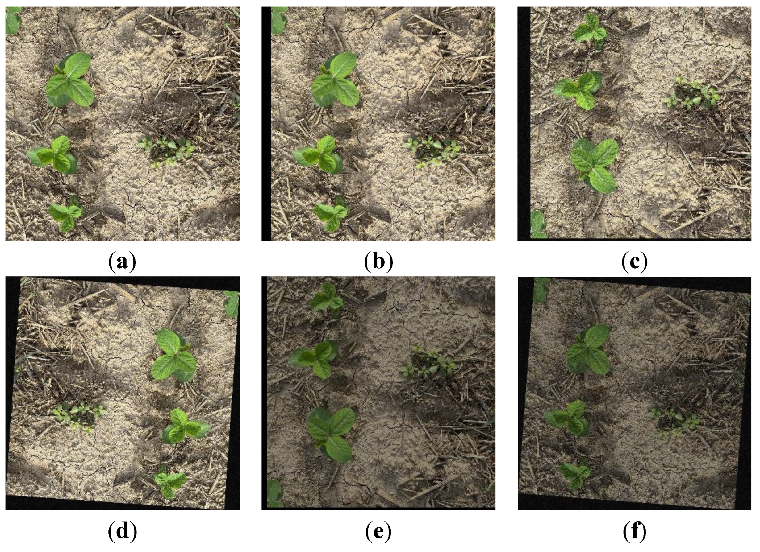
An example of data enhancement is shown in Figure 3. The data preprocessing module obtains five images to simulate the growth of soybean seedlings and weeds under complex natural conditions by applying data enhancement methods such as translation, shear, flip, rotation, and addition noise to the original images. This way, a larger sample dataset can be conveniently obtained in the laboratory.
Through data preprocessing, we obtain the dataset required to train the model; however, the size of the input images (3,024*3,024) does not match the target input size for the recognition module (640*640). Thus, we adopt the adaptive image scaling technique (Letterbox) to transform an input image of arbitrary size into 640*640, which well matches the model input and the target recognition module, thereby making our SWIM model handle more images of various sizes obtained from different devices.
In this article, the original data is first divided into a training set (training set + validation set) and a test set, and the training set is enhanced to obtain the dataset used in this article.

2.2. Methods

2.2.1. Design of a Computational Complexity-Driven Model for Soybean Seedling and Weed Identification

The goal of our research is to enable the deployment of soybean seedling and weed recognition models to terminal devices for agricultural information technology, such as weeding robots, real-time measurement and control systems for field management drones, and so on. Typically, the image acquisition systems deployed in these devices capture images that are noisy, incomplete, or distorted, and the onboard information processing systems have limited memory and computational speed. Therefore, the premise that terminal devices can respond accurately and quickly is that the computational space complexity and computational time complexity of soybean seedling and weed identification algorithms are low, while the identification accuracy is high. We have confirmed through experiments (yolov5-6.1/runs/detect/YOLOv5n Identification) that the YOLOv5n model cannot identity soybean seedlings and weeds without undergoing transfer learning. However, after few-shot training, the identification performance of this base model reached 91.4%, with a fast convergence rate. Therefore, this article aims to design a soybean seedling and weed identification model (SWIM) suitable for agricultural information terminal devices by leveraging the computational complexity-driven approach based on the research of the mature algorithm YOLOv5n. The specific methods are as follows.
  • Computational Complexity-driven CSPPC Module
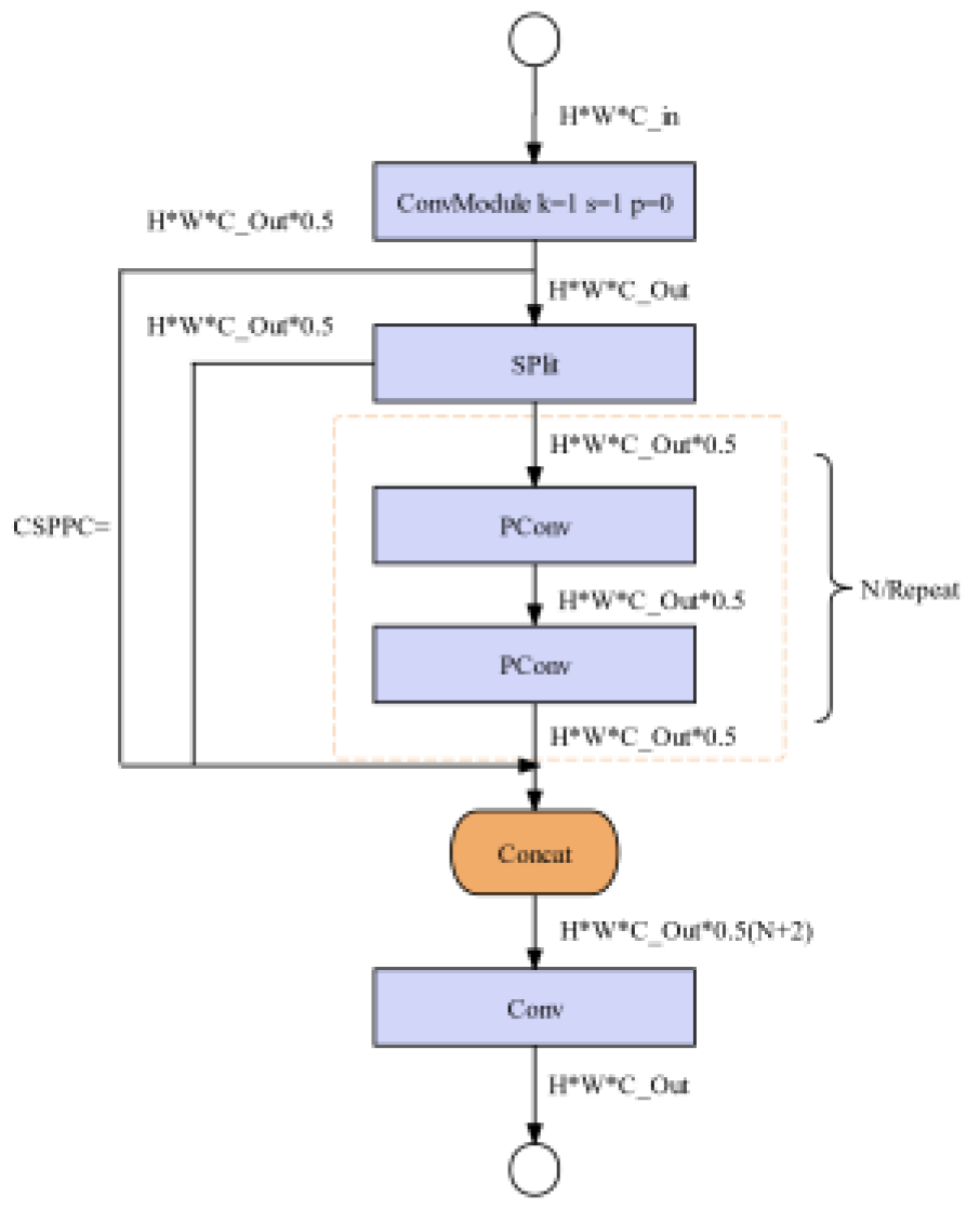
The design philosophy of the CSPPC module is based on PConv [34] and incorporates DualConv [35]. PConv only extracts features from a subset of input channels. In the identification of soybean seedlings and weed images, CSPPC replaces all C3 modules in the YOLOv5n network to obtain the model C_YOLOv5n. Experiments have shown that the computational space complexity decreases from 1.77M to 1.27M, and the computational time complexity decreases from 4.2GFLOPs to 3.0GFLOPs, significantly reducing the computational complexity. The structure of the CSPPC module is shown in Figure 4.
2.
Computational Complexity-driven Ghost Module
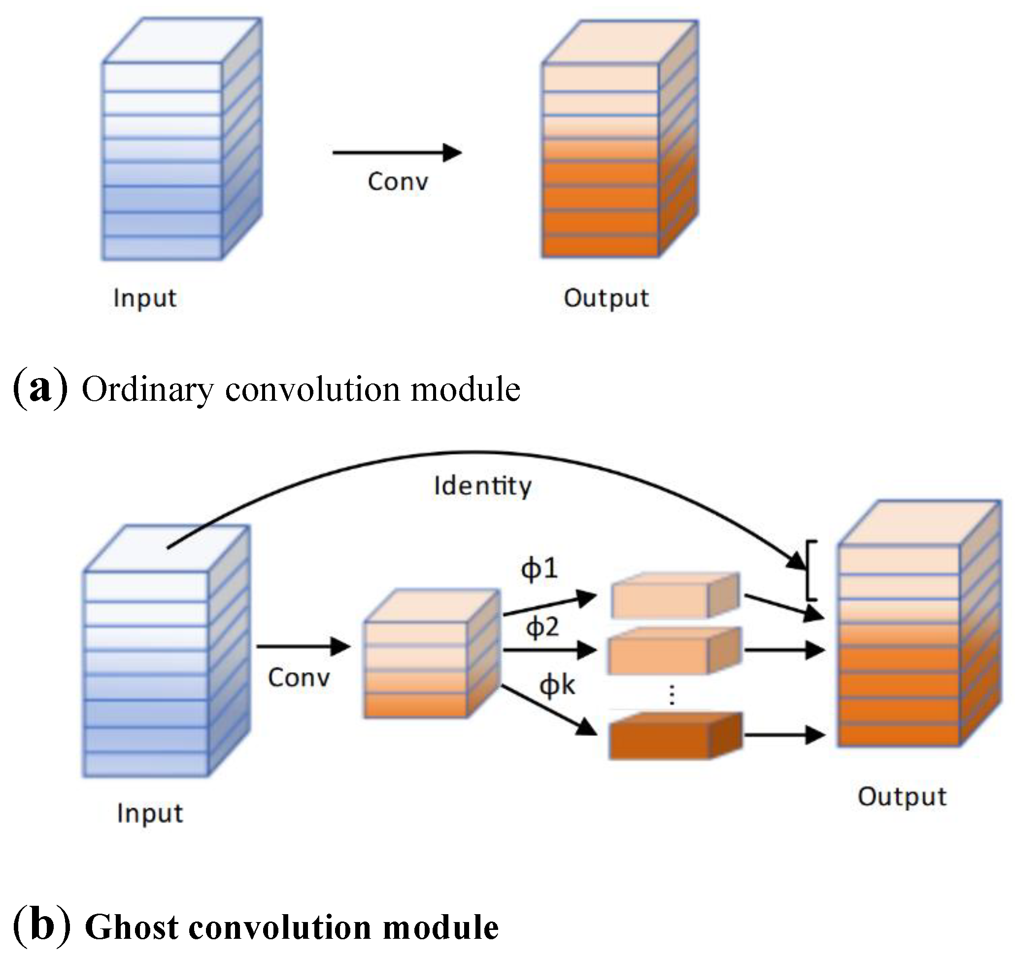
The Ghost module is the core component of GhostNet, which generates feature maps through linear transformation to obtain more information. In the identification of soybean seedlings and weed images, we replaced all CBS modules in C_YOLOv5n with Ghost modules and named it model SWIM_T. Experiments have shown that the computational space complexity changes from 1.77M to 0.97M, and the computational time complexity changes from 4.2 GFLOPs to 2.3 GFLOPs, further reducing the computational complexity of the model. Figure 5 is a schematic diagram of ordinary convolution and Ghost convolution modules.
3.
MLCA Attention Mechanism
After performing the above two lightweight operations on the weed recognition model, the computational space complexity and time complexity of the model are significantly reduced, but at the same time, the recognition accuracy of the model will also decrease. Observing the images of soybean seedlings during the seedling stage, we found that the complexity of the images comes from the complex background, as well as the mutual occlusion between soybean seedlings, between soybean seedlings and weeds, and between weeds. This means that there are interactions between features in different spaces. Therefore, adding an attention mechanism to the model can effectively improve its recognition accuracy.
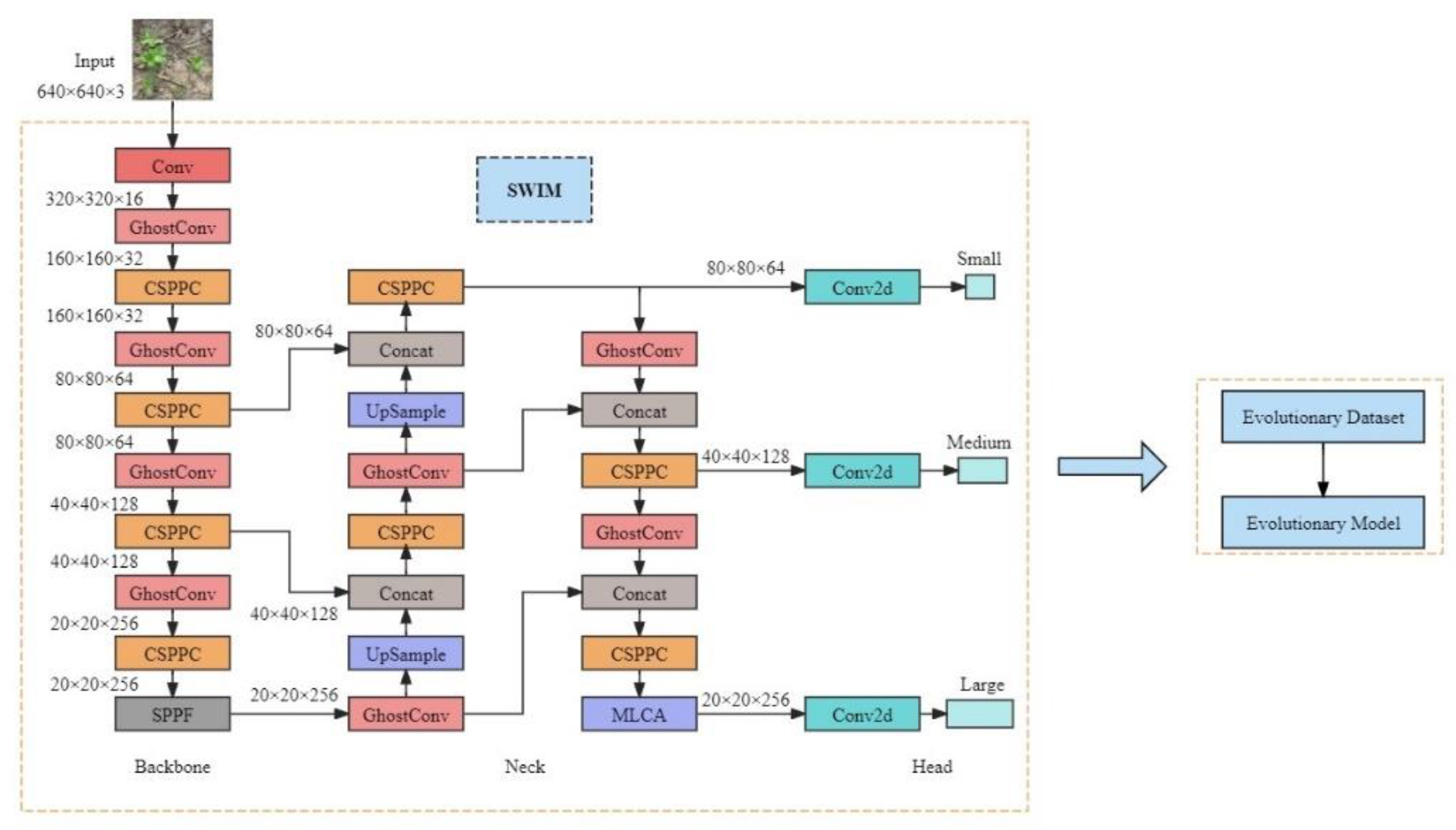
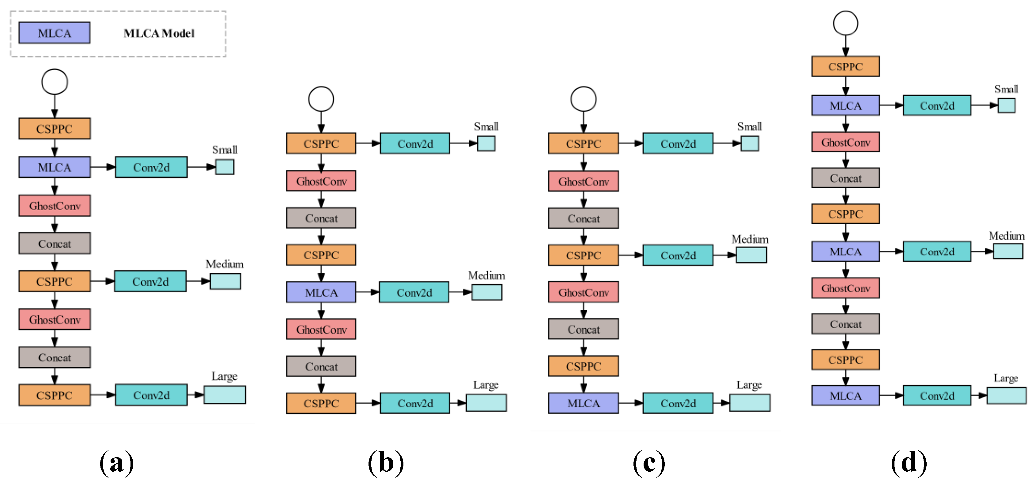
As shown in Figure 7, this article introduces the MLCA mechanism after the CSPPC module at the end of the feature fusion section to improve the feature extraction ability of weeds and soybean seedlings, thereby compensating for the accuracy loss. Meanwhile, due to the limited number of parameters and floating-point operations in MLCA, the addition of this module will not significantly increase the space complexity and time complexity of the model.
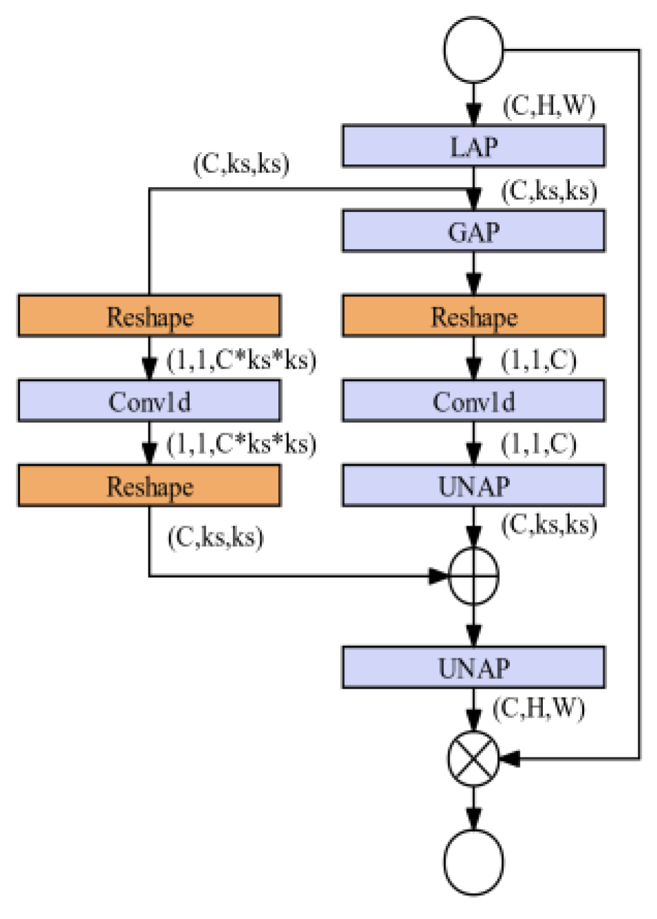
The basic principle of MLCA is to enhance the representation capability of the model by simultaneously integrating channel information and spatial information, local information, and global information. The MLCA network structure is shown in Figure 6.
As shown in Figure 6, Local Average Pooling (Abbr. LAP) [36] and Global Average Pooling (Abbr. GAP) [37] are key preprocessing steps. LAP improves the perception ability of target local information by aggregating the characteristics of soybean seedlings and weeds in local areas; GAP aggregates the information of the entire feature map and captures the global statistical information of the target. Conv1d [38] rearranges the feature information of soybean seedlings and weeds by compressing feature channels; Then, the locally pooled features are combined with the input features of the original soybean seedlings and weeds through a multiplication operation; The globally pooled features are fused with local features through an "addition" operation. Finally, the feature maps that have undergone local and global processing are restored to their original spatial dimensions through Un-Average Pooling (Abbr. UNAP) [39] operation.
Considering that most of the recognition targets in the image dataset of this article are large targets, they are placed at the output position of the large target detection layer based on experience. Experiments have shown that the recognition accuracy of the model is improved at this position. It can be seen that the module can compensate for the recognition accuracy of the model without significantly increasing the spatial and temporal complexity of the model. The network structure of SWIM is shown in Figure 7.
Figure 7. Network structure of SWIM.
Preprints 115627 g007

2.2.2. Model Evolution

In practical applications, the image acquisition systems of agricultural intelligent terminals are different from each other, and the working farmland conditions are not the same, which increases the error rate of the model when detecting actual images. Therefore, it is necessary to design an evolutionary model that can adapt to changes in the field environment and different equipment, and finetune the model parameters to improve identification performance.
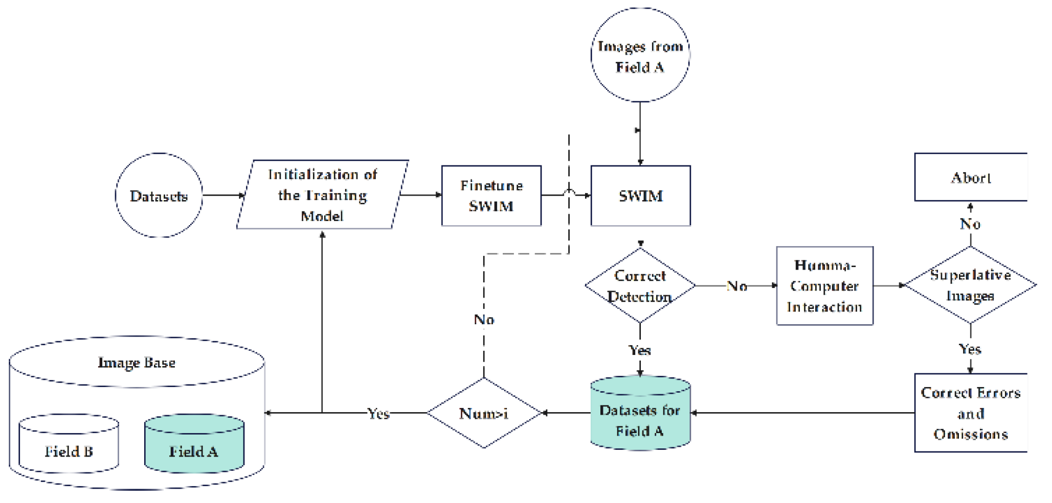
The identification system designed in this study, named ESWIM, operates as shown in Figure 8. Images collected from Field A are detected using the SWIM model. If all identification targets are correctly identified in the detected image, the system adds the image and its annotations to the sample dataset of Field A. If there are any missed or incorrect targets in the detected image, human-computer interaction ensues: if the image has serious quality issues, it is deleted; otherwise, the operator corrects the errors and omissions in the detected image, and the corrected image and labels are added to the sample dataset of Field A. Once the sample dataset of Field A reaches a certain size, the parameters of the SWIM model are fine-tuned using this dataset, allowing the identification model to continuously evolve in its work. At the same time, the datasets for soybean seedlings and weeds are also continuously evolving, providing rich and accurate diversified data for subsequent large-scale intelligent management of farmland. The value of i is adjusted according to different geographical environments and actual crops, enabling the model to quickly obtain optimal model parameters. This allows the evolutionary system designed in this article to be applied to various crops.

2.2.3. Network Model Training

The experimental hardware environment is a 10-core CPU model AMD EPYC 7443 24-Core Processor workbench with 50GB of RAM and an NVIDIA A40 graphics card. The construction of the weed recognition model is developed using Python 3.8, and the deep learning framework is selected as Pytorch, and the development tool is Pycharm ver. 2022.3. The programming language is Python.
In order to obtain optimal model parameters for the soybean seedlings and weed model while also speeding up convergence during training, we determined the key parameter values for model training through multiple experiments, as shown in Table 2.
The cosine annealing algorithm is used in model training to adjust the learning rate, and the original non-maximal suppression (NMS) is used to suppress the detection of the redundant frames and select the best prediction frame.

2.2.4. Trial Evaluation Indicators

In order to evaluate whether the model designed in this article can be deployed on smart agricultural equipment terminals and perform effective real-time work in complex field environments, it is necessary to evaluate the space complexity Params and time complexity Floating-Point Operations (FLOPs) of the model. To study the recognition accuracy of each target, it is necessary to calculate the Average Pecision (AP), Precision, and Recall of each category; To evaluate the overall recognition accuracy of the model, it is necessary to calculate the Mean Average Precision (mAP), Overall Precision (Over_Precision), and Overall Recall (Over_Recall).
To calculate the above performance metrics, we set the identification target space as:
Φ = { s o y b e a n = 1 , m a c h i x i a n = 2 , d a w a n h u a = 3 , c i e r c a i = 4 , l i = 5 , m a t a n g = 6 , t i e x i n a c a i = 7 , n o n _ t a r g e t = 8 } .
Therefore, if the current positive sample is i as i ∈ [1,7], the current negative sample is j as j ∈ [1,8] while ij.
Let:
T P i : classifying class i as class i, True Positive (TP) represents the model correctly identifying the soybean seedlings and 6 species of weeds;
F P i j : misclassifying class j as class i; For example, if i=3 is for “dawanhua”, means that “li” was mistakenly identified as the target “dawanhua”;
F N i j : misclassifying class i as class j; For example, if i=3 is for “dawanhua”, means that the target “dawanhua” was mistakenly identified as “li”;
So, the Overall True Positive (Over_TP) which is the total number of correctly classified samples detected by the model is:
O v e r _ T P = i = 1 7 T P i .
The Overall False Positive (Over_FP) which is the total number of negative samples that have been wrongly classified as positive samples by the model is:
O v e r _ F P = i = 1 7 j = 1 8 F P i j , i j .
The Overall False Negative (Over_FN) which is the total number of positive samples that have been wrongly classified as negative samples by the model is:
O v e r _ F N = j = 1 8 i = 1 7 F N i j ,   i j .
So, the performance metrics of the model are calculated as follows:
  • Calculation of performance metrics for each category of target
Precision(i), which is the ratio of the correctly classified predictive bounding box for each category i, is:
Precision i = T P i T P i + j = 1 8 F P i j × 100 % ,   i j .
Recall(i), which is the ratio of correctly classified labeling bounding box for each category i, is:
Recall i = T P i T P i + j = 1 8 F N i j × 100 % ,   i j .
The accuracy A P i for each category i is:
A P i = k = 0 n 1 [ R e c a l l i ( k ) - R e c a l l i ( k + 1 ) ] · ( m a x ) P r e c i s i o n i k × 100 % .
2.
Calculation of overall performance metrics for the model
Similarly, we can obtain the formula for calculating the overall performance metrics of the model as follows:
Over _ Precision = O v e r _ T P O v e r _ T P + O v e r _ F P × 100 % ,
Over _ Recall = O v e r _ T P O v e r _ T P + O v e r _ F N × 100 % ,
A P = k = 0 n 1 [   Recall ( k ) - Recall ( k + 1 ) ] · ( m a x ) P r e c i s i o n k × 100 % .
As there are m categories that need to be identified in the soybean seedling image in the seedling stage, the mAP is:
m A P = i = 1 m A P i m × 100 % .
When m = 6, it represents the average accuracy of 6 types of weeds; when m = 7, it represents the average accuracy of soybean seedlings and 6 types of weeds.

3. Results

3.1. Ablation Experiment and Analysis of SWIM Model

In this article, we constructed the SWIM model based on YOLOv5n, a framework with excellent generalization performance trained on over one million image samples. We simulated soybean seedlings and weeds in natural environments using a small dataset and reasonable image enhancement techniques to expand the training dataset. Essentially, we finetuned the model parameters to ensure that the model's performance in detecting soybean seedlings and weeds meets application requirements. This section designed ablation experiments to verify that the model has low computational space and time complexity, high accuracy, and can be deployed on smart agricultural terminals with low storage capacity. At the same time, by testing the results of SWIM under different datasets, we analyzed the model's few-shot finetuning performance and the considerations of system evolution datasets.

3.1.1. Experiment on Computational Space Complexity and Time Complexity

To verify that the soybean seedling and weed identification model developed in this study can significantly reduce computational space complexity and time complexity without compromising accuracy, the following ablation experiment was conducted (Article Trial):
Model 1: YOLOv5n, the baseline model;
Model 2: C_YOLOv5n, C3 module in YOLOv5n is replaced with the CSPPC module;
Model 3: G_YOLOv5n, the CBS module in YOLOv5n is replaced with GhostConv;
Model 4: Soybean and Weed Identification Model Trail (SWIM_T), replacing the CBS module in C_YOLOv5n with GhostConv;
Experimental dataset: 7,482 images, with 1,247 original images and another 6,235 images generated from the original dataset using data augmentation methods.
The performance metrics of the four models, as obtained through experiments, are shown in Table 3.
As can be seen from Table 3, the computational space complexity and time complexity of SWIM_T are significantly lower than those of YOLOv5n. By comparing the performance parameters with the control model, the number of parameters in the C_YOLOv5n decreased by 0.50M and the FLOPs decreased by 1.2 GFLOPs, while the G_YOLOv5n parameters decreased by 0.30M and the FLOPs decreased by 0.6 GFLOPs. It can be seen that the effect of replacing the C3 module with the CSPPC module in YOLOv5n is significantly better than replacing the CBS module with the Ghost module. SWIM_T compared with the control model, the number of parameters is reduced by 0.80M, the computational complexity is reduced by 1.9 GFLOPs, and the computational complexity and time complexity are reduced by nearly 50%. It can be seen that the SWIM_T model significantly reduces the computational space complexity and time complexity of the control model, so that the model can be deployed on terminals with small memory capacity and can run at high speed.
The mAP of the above three models decreased by 1.8% compared with the control model, so it is necessary to compensate for the accuracy of the model.

3.1.2. Accuracy Compensation Experiments

According to the above principle, the accuracy can be improved by adding MLCA with a self-attention mechanism and low computational complexity. Since MLCA is a plug-and-play module, that can be directly placed anywhere in the network architecture, in order to explore the influence of MLCA modules on network performance at different locations in the network, the following models and experiments are designed:
Model 5: SWIM_S, MLCA is added to the tail of the CSPPC module SWIM_T the small target detection layer;
Model 6: SWIM_M, MLCA is added to the tail of the CSPPC module of the target detection layer in the SWIM_T;
Model 7: SWIM, MLCA is added to the tail of the CSPPC module SWIM_T large target detection layer;
Model 8: SWIM_A, MLCA is added to the tail of the CSPPC module of the three object detection layers of the SWIM_T.
The different positions of MLCA in the network are shown in Figure 9.
The performance metrics of the four models, with the experimental dataset remaining unchanged, are shown in Table 4.
According to Table 4, SWIM has the best accuracy. The experimental results are shown in (Article Trial).
In summary of Table 3 and Table 4, by comparing the performance indicators of SWIM and SWIM_T, it can be known that the former has an mAP improvement of 1.9%, reaching 90.3%, without significantly increasing the model's computational space and time complexity. The accuracy loss of the model is effectively compensated.

3.1.3. Comparative Experiment on Dataset Augmentation and Partitioning Order

To investigate the influence of the order of enhancing and partitioning original data on SWIM model training, 445 images are randomly selected uniformly from 1,336 original images. The experimental design is as follows:
Scheme 1: First, enhance 445 images to 5,486 images using a data augmentation module. Then divide them into training set (training set + validation set) and test set in a ratio of 3:1:1. Obtain the dataset 1 that is first augmented and then divided.
Scheme 2: First, divide the 445 original images into a training set and a validation set in a ratio of 3:1. Then, enhance them to 5486 images using the same ratio. Obtain the dataset 2 that is first divided and then augmented.
After extracting 445 images from the original 1,336 images, 89 images were randomly selected as the application scenario test set for performance evaluation of the two schemes. The SWIM model was used for training, and the experimental (Number Datasets Trial) results are shown in Table 5.
As can be seen from Table 5, enhancing before partitioning results in a high correlation among the three sets, leading to excessively high mAP of the validation set, AP of soybean seedlings, and AP of weeds. However, on the test set, the AP of soybean seedlings slightly decreases, the AP of weeds drops by 22.2%, and the total mAP also decreases by 19.8%, indicating that the experimental results of the validation set are artificially high. The results of enhancing after partitioning show that there is no significant deviation between the validation set and the test set. This proves that the dataset enhanced after partitioning is more in line with the law of large numbers, and the dataset in this article will also be generated in the way of partitioning before enhancement.

3.1.4. Comparative Experiment on Datasets with Various Enhancement Ratios

To explore the impact of data volume on model training and the effectiveness of data augmentation modules, an experiment was designed: 89 images were randomly selected from 1,336 original images as the test set to verify the performance of the model. The remaining 1,247 images were divided into training and validation sets at a ratio of 3:1, and then augmented n times. These datasets with different dataset sizes were used for training and validation. The control model was YOLOv5n, and the experimental model was SWIM. Training dataset design: training set (1,247 original images + n*1,247 augmented images), application scenario test set (89 original images). The parameter design of the training model was based on the same training strategy and the same sample set, which could find the optimal training result for both models. The experimental (Number Datasets Trial) results are shown in Figure 10.
The figure shows that the performance metrics for both the validation and test results of SWIM generally exhibit an upward trend, while YOLOv5n shows a slight downward trend. As seen in (a), under the training of the SWIM model, the AP for soybean seedlings in both the validation and test sets remains stable and high. The mAP closely correlates with the AP for weeds, generally changing in tandem with it. Therefore, selecting the optimal number of datasets for this model based on the AP for weeds yields the best model parameters. Similarly, this experimental phenomenon is observed in (b). According to (a) and (c), when the original data images (1,247 images) are enhanced by a factor of 5, that is, with a total data volume of 7,482 images, both the test set mAP and the AP for weed recognition are optimal, with an mAP of 90.3% and an AP for weed recognition of 89.3%. As seen in (b) and (d), the optimal number of datasets for the YOLOv5n model is when enhanced by a factor of 1.
In summary, under the SWIM model training, the dataset is proportional to the number of data provided that meets the assumption of independent and identically distributed. However, there is a limit to the augmentation factor, otherwise, the model will be affected when the total dataset reaches a certain amount, and the accuracy will decrease instead. It also proves that using data augmentation algorithms to perform translation, rotation, and Gaussian noise addition on the original data can indeed increase the diversity of the sample space. According to the experimental results, data augmentation methods are feasible, but subsequent adjustments to the parameters of the data augmentation module are needed based on the specific complex natural environment of soybean fields so that the data augmentation module can more realistically mimic the plant morphology in complex natural environments.

3.2. Evolutionary Experiment

To verify the practical application of the model in this article on the evolutionary dataset in natural environments, 50 images of soybeans and weeds at the seedling stage were selected for recognition. The misidentified and missed identification annotation files in the recognition results were manually corrected, and then these modified label files and images were placed into the original dataset (1,247 original images + 5*1247 enhanced images) to obtain an evolutionary dataset, which was then used for training. The trained new model ESWIM was used for recognition testing, and the comparison results with the control model SWIM are shown in Table 6:
After comparing the results, it was found that the evolved ESWIM model exhibited superior performance in the test results. The recognition accuracy of soybean seedlings and six types of weeds improved to varying degrees, with a 0.4% increase in mAP, a 0.8% increase in soybean seedling AP, and a 0.3% increase in weeds AP. In terms of training duration, the ESWIM model requires less training time compared to the SWIM model, demonstrating that the ESWIM system can quickly adjust its identification system during device operation to achieve target recognition tasks in various environments. Although the improvement is not significant, it still effectively demonstrates the feasibility and effectiveness of using evolutionary datasets for model evolution, providing a reference for future research. This article has practical applicability, and it can be seen that evolutionary datasets can indeed improve the recognition accuracy of the model to a certain extent. Therefore, it can be proved that with the continuous practical application of this model, the diversity of plant species and growth status in the evolutionary dataset will continue to increase. The model will also continue to learn, further improving recognition accuracy and efficiency. The application of the evolutionary database can provide certain reference value for subsequent recognition of soybean seedlings and weeds, as well as other weed detection fields.

4. Conclusions and Outlooks

4.1. Conclusions

To realize the real-time recognition task of soybean seedlings and weeds in a soybean seedling field on an agricultural intelligent terminal device, this article constructs a real-time computational complexity-driven evolutionary identification system, ESWIM, under few-shot training for recognizing weeds and soybean seedlings. The model ESWIM constructed in this study is obtained through two processes. Firstly, using YOLOv5n as the base model and driven by the idea of reducing computational complexity, Ghost, CSPPC, and MLCA modules are introduced to construct SWIM, a soybean seedling and weed identification model with low complexity but no loss of recognition accuracy. In practical applications, we use human-computer interaction to process and make decisions on the identification images in our work to build an evolutionary dataset of specific farmland, which is used by the evolutionary strategies to quickly and iteratively update the SWIM model parameters to obtain an ESWIM system that adapts to field-specific scenarios in real-time.
In the research of this article, we try to find a way to use the base model to build new models driven by complexity reduction, which can be adapted to different tasks of detecting farmland plants under the training of few-shot datasets. To this end, we designed and conducted a large number of experiments, trying to think and practice actively in terms of the driving orientation of model building, the way of thinking about data processing, and how scientific experiments should be designed in order to get faster conclusions during model training. For example, we design the comparison experiments between the base model to directly recognize the target object of this study and the few-shot transfer learning model, and choose the base model with good generalization performance and strong migration ability. We designed ablation and comparison experiments to verify the feasibility and effectiveness of the proposed recognition model. We obtained the enhancement algorithm by analyzing the farmland landscape, the weather and image acquisition methods, and the status of equipment fieldwork during the growing period of soybean seedlings in this study, and used the collected few-shot for appropriate data enhancement to obtain the soybean seedlings and weeds dataset used in model training. The dataset thus obtained contains both the original samples and the generated diversity images that can effectively simulate the actual images and can alleviate the problem of significant imbalance in the number of targets. Before training, the targets for object identification in each image are counted, and under the goal of short training time and the best possible results, and considering that data enhancement has double the time costs of enhancement and training, we first design experiments that do not enhance the dataset but change the batch-size, and find that the optimal batch-size is 16. On the basis of this, we design experiments on data partitioning and data enhancement order and find that the data enhancement order used in this study is 16. We found that using division before enhancement in this study can make the validation error more reflective of the testing error. During the experimental process, we will analyze the performance of various classes and the overall performance of each experiment, and analyze the performance of the identification model, so as to provide guidance for the next experiment.
The system proposed in this article was experimented by the above experimental methods and experiments using self-constructed soybean seedling and weed datasets. The experimental results show that relative to the base model, the computational space complexity and time complexity of the identification model SWIM decreased by 45.19% and 42.86%, respectively, and the average accuracy of the model increased by 0.1% to 90.3%. The AP for each weed was also above 80%, which meets the accuracy criteria mentioned previously. In order to study the evolution of the ESWIM system, we used a complex image of this farmland to experiment with building an evolutionary dataset through human-computer interaction for a specific field at work and iterating the SWIM model after reaching a certain sample. The designed experiments prove that the average accuracy of our model increases by another 0.4% to 90.7%, which enables the recognition accuracy of this identification system to be increased, thus making the deployed device adaptable in real-time to the detection task of this farmland. During the experimental process, we will analyze the performance of the identification model by analyzing the performance of the various classes and the overall performance of each experiment, for example, the identification rate of the Herb of Common Crabgrass weed has been relatively low in this study, which may be related to the small number of Herb of Common Crabgrass samples as well as the morphology of this weed. Therefore, it is proposed to obtain more image samples of Herb of Common Crabgrass weed in multiple scenarios in the subsequent study to fully learn its morphological features and improve the problem of missed identification and misidentification.
In summary, this article constructs the soybean seedling stage farmland weed identification and evolution system ESWIM through the few-shot data set of reasonable data enhancement and migration training, can be deployed to the corresponding agricultural intelligent terminal equipment with limited computational resources, not only can monitor the identification of soybean seedling stage of the farmland weeds and real-time evolution, but also in the work of the establishment of a specific farmland data and information base, to provide data and information support for precision agriculture information support. At the same time, the model construction and training analysis of this article can provide ideas for research in the same field.

4.2. Outlooks

Although this article is a study of major weeds in soybean farmland in a region of Henan Province, the constructed system and research methodology can provide good research ideas for detection tasks in the field management of other crop species. According to our current research, the follow-up work is proposed to be carried out in the following three aspects: firstly, because it is the image of the soybean seedling stage, the image samples of normal soybean fields will inevitably have the sample imbalance of soybean seedlings in the majority and weeds in the minority. Therefore, in the follow-up research work, how to use a few-shot of the original image, using the function of computer image generation, to generate polymorphic images to improve the sample imbalance phenomenon, so that the model can be effectively trained, but does not lead to the collapse of the model; secondly, adapted to different plots of real-time systems for crop weed identification, so it is necessary to study the system with strong migratory learning ability and rapid training methods; thirdly, deployment of self-learning ability of the Development of intelligent equipment terminals for agriculture.

Author Contributions

Conceptualization, Shuyang.Yan., Yaling.Lu. and Tianyi.Li.; methodology, Shuyang.Yan., Yaling.Lu., Zhen.Huang. and Zhigang.Hu.; software, Shuyang.Yan.; validation, Shuyang.Yan. and Yaling.Lu.; formal analysis, Shuyang.Yan. and Yaling.Lu.; investigation, Shuyang.Yan. and Yaling.Lu.; resources, Shuyang.Yan. and Yaling.Lu.; data curation, Shuyang.Yan., Yaling.Lu. and Yi.Rong.; writing—original draft preparation, Shuyang.Yan., Yaling.Lu. and Tianyi.Li.; writing—review and editing, Shuyang.Yan. and Tianyi.Li.; visualization, Shuyang.Yan.; supervision, Yaling.Lu.; All authors have read and agreed to the published version of the manuscript.

Funding

This research received no external funding.

Institutional Review Board Statement

Not applicable.

Informed Consent Statement

Not applicable.

Data Availability Statement

Conflicts of Interest

The authors declare no conflicts of interest.

References

  1. Liu, Z.; Ying, H.; Chen, M.; Bai, J.; Xue, Y.; Yin, Y.; Batchelor, W.D.; Yang, Y.; Bai, Z.; Du, M.; et al. Optimization of China’s maize and soy production can ensure feed sufficiency at lower nitrogen and carbon footprints. Nature Food 2021, 2, 426–433. [Google Scholar] [CrossRef] [PubMed]
  2. Yu, H.; Men, Z.; Bi, C.; Liu, H. Research on Field Soybean Weed Identification Based on an Improved UNet Model Combined With a Channel Attention Mechanism. Frontiers in Plant Science 2022, 13. [Google Scholar] [CrossRef]
  3. Klerkx, L.; Jakku, E.; Labarthe, P. A review of social science on digital agriculture, smart farming and agriculture 4.0: New contributions and a future research agenda. NJAS - Wageningen Journal of Life Sciences 2019, 90-91, 100315–100315. [Google Scholar] [CrossRef]
  4. Liu, B.; Li, R.; Li, H.; You, G.; Yan, S.; Tong, Q. Crop/Weed Discrimination Using a Field Imaging Spectrometer System. Sensors 2019, 19, 5154. [Google Scholar] [CrossRef]
  5. Nahina, I.; Mamunur, R.M.; Santoso, W.; ChengYuan, X.; Ahsan, M.; A., W.S.; Steven, M.; Mostafizur, R.S. Early Weed Detection Using Image Processing and Machine Learning Techniques in an Australian Chilli Farm. Agriculture 2021, 11, 387–387. [Google Scholar] [CrossRef]
  6. Zuoyu, Z.; Qian, T.; Wu, L. Research on plant image classification method based on convolutional neural network. Internet of things Technology 2020, 10, 72–75. [Google Scholar] [CrossRef]
  7. Simonyan, K.; Zisserman, A. Very deep convolutional networks for large-scale image recognition. arXiv 2014, arXiv:1409.1556. [Google Scholar] [CrossRef]
  8. Long, J.; Shelhamer, E.; Darrell, T. Fully convolutional networks for semantic segmentation. In Proceedings of the Proceedings of the IEEE conference on computer vision and pattern recognition, 2015; pp. 3431–3440. [CrossRef]
  9. Desheng, W.; Yan, X.; Jianping, Z.; Xiangpeng, F.; Yang, L. Weed identification method based on deep convolutional neural network and color migration under the influence of natural illumination. China Sciencepaper 2020, 15. [Google Scholar]
  10. He, C.; Wan, F.; Ma, G.; Mou, X.; Zhang, K.; Wu, X.; Huang, X. Analysis of the Impact of Different Improvement Methods Based on YOLOV8 for Weed Detection. Agriculture 2024, 14, 674. [Google Scholar] [CrossRef]
  11. Hussain, M. YOLO-v1 to YOLO-v8, the rise of YOLO and its complementary nature toward digital manufacturing and industrial defect detection. Machines 2023, 11, 677. [Google Scholar] [CrossRef]
  12. Zhang, X.; Cui, J.; Liu, H.; Han, Y.; Ai, H.; Dong, C.; Zhang, J.; Chu, Y. Weed identification in soybean seedling stage based on optimized Faster R-CNN algorithm. Agriculture 2023, 13, 175. [Google Scholar] [CrossRef]
  13. Ren, S.; He, K.; Girshick, R.; Sun, J. Faster r-cnn: Towards real-time object detection with region proposal networks. Advances in neural information processing systems 2015, 28. [Google Scholar] [CrossRef] [PubMed]
  14. Liu, W.; Anguelov, D.; Erhan, D.; Szegedy, C.; Reed, S.; Fu, C.-Y.; Berg, A.C. Ssd: Single shot multibox detector. In Proceedings of the Computer Vision–ECCV 2016: 14th European Conference, Amsterdam, The Netherlands, 11–14 October 2016; Proceedings, Part I 14. pp. 21–37. [Google Scholar] [CrossRef]
  15. Bochkovskiy, A.; Wang, C.-Y.; Liao, H.-Y.M. Yolov4: Optimal speed and accuracy of object detection. arXiv 2020, arXiv:2004.1093. [Google Scholar] [CrossRef]
  16. Jocher, G.; Chaurasia, A.; Stoken, A.; Borovec, J.; Kwon, Y.; Michael, K.; Fang, J.; Yifu, Z.; Wong, C.; Montes, D. ultralytics/yolov5: v7. 0-yolov5 sota realtime instance segmentation. Zenodo 2022. [Google Scholar]
  17. Lou, F.; Lu, Y.; Wang, G. Design of a Semantic Understanding System for Optical Staff Symbols. Applied Sciences 2023, 13, 12627. [Google Scholar] [CrossRef]
  18. Wang, B.; Yan, Y.; Lan, Y.; Wang, M.; Bian, Z. Accurate detection and precision spraying of corn and weeds using the improved YOLOv5 model. IEEE Access 2023, 11, 29868–29882. [Google Scholar] [CrossRef]
  19. Deng, J.; Zhong, Z.; Huang, H.; Lan, Y.; Han, Y.; Zhang, Y. Lightweight Semantic Segmentation Network for Real-Time Weed Mapping Using Unmanned Aerial Vehicles. Applied Sciences 2020, 10, 7132. [Google Scholar] [CrossRef]
  20. Wang, S.; Wang, S.; Zhang, H.; Wen, C. Soybean field weed recognition based on light sum-product networks and UAV remote sensing images. Journal of Agricultural Engineering 2019, 35, 89–97. [Google Scholar] [CrossRef]
  21. Wang, C.-Y.; Liao, H.-Y.M.; Wu, Y.-H.; Chen, P.-Y.; Hsieh, J.-W.; Yeh, I.-H. CSPNet: A new backbone that can enhance learning capability of CNN. In Proceedings of the Proceedings of the IEEE/CVF conference on computer vision and pattern recognition workshops, 2020; pp. 390–391191111929.
  22. Ren, D.; Yang, W.; Lu, Z.; Chen, D.; Su, W.; Li, Y. A Lightweight and Dynamic Feature Aggregation Method for Cotton Field Weed Detection Based on Enhanced YOLOv8. Electronics 2024, 13, 2105. [Google Scholar] [CrossRef]
  23. Cui, C.; Gao, T.; Wei, S.; Du, Y.; Guo, R.; Dong, S.; Lu, B.; Zhou, Y.; Lv, X.; Liu, Q. PP-LCNet: A lightweight CPU convolutional neural network. arXiv 2021, arXiv:2109.15099. [Google Scholar] [CrossRef]
  24. Liu, Y.; Shao, Z.; Teng, Y.; Hoffmann, N. NAM: Normalization-based attention module. arXiv 2021, arXiv:2111.12419. [Google Scholar] [CrossRef]
  25. Razfar, N.; True, J.; Bassiouny, R.; Venkatesh, V.; Kashef, R. Weed detection in soybean crops using custom lightweight deep learning models. Journal of Agriculture and Food Research 2022, 8, 100308. [Google Scholar] [CrossRef]
  26. He, K.; Zhang, X.; Ren, S.; Sun, J. Deep residual learning for image recognition. In Proceedings of the Proceedings of the IEEE conference on computer vision and pattern recognition, 2016; pp. 770–778. [CrossRef]
  27. Howard, A.G.; Zhu, M.; Chen, B.; Kalenichenko, D.; Wang, W.; Weyand, T.; Andreetto, M.; Adam, H. Mobilenets: Efficient convolutional neural networks for mobile vision applications. arXiv 2017, arXiv:1704.04861. http://arxiv.org/abs/1704.04861.
  28. LeCun, Y.; Boser, B.; Denker, J.S.; Henderson, D.; Howard, R.E.; Hubbard, W.; Jackel, L.D. Backpropagation applied to handwritten zip code recognition. Neural computation 1989, 1, 541–551. [Google Scholar] [CrossRef]
  29. Liu, R.-M.; Su, W.-H. APHS-YOLO: A Lightweight Model for Real-Time Detection and Classification of Stropharia Rugoso-Annulata. Foods 2024, 13, 1710. [Google Scholar] [CrossRef]
  30. Han, K.; Wang, Y.; Tian, Q.; Guo, J.; Xu, C.; Xu, C. Ghostnet: More features from cheap operations. In Proceedings of the Proceedings of the IEEE/CVF conference on computer vision and pattern recognition, 2020; pp. 1580–1589. http://arxiv.org/abs/1911.11907.
  31. Wan, D.; Lu, R.; Shen, S.; Xu, T.; Lang, X.; Ren, Z. Mixed local channel attention for object detection. Engineering Applications of Artificial Intelligence 2023, 123, 106442. [Google Scholar] [CrossRef]
  32. Alhazmi, K.; Alsumari, W.; Seppo, I.; Podkuiko, L.; Simon, M. Effects of annotation quality on model performance. In Proceedings of the 2021 International Conference on Artificial Intelligence in Information and Communication (ICAIIC), 13-16 April 2021; pp. 063–067. [Google Scholar] [CrossRef]
  33. Huang, F.; Wang, J.; Yi, P.; Peng, J.; Xiong, X.; Liu, Y. SCSQ: A sample cooperation optimization method with sample quality for recurrent neural networks. Information Sciences 2024, 674, 120730. [Google Scholar] [CrossRef]
  34. Chen, J.; Kao, S.-h.; He, H.; Zhuo, W.; Wen, S.; Lee, C.-H.; Chan, S.-H.G. Run, don't walk: chasing higher FLOPS for faster neural networks. In Proceedings of the Proceedings of the IEEE/CVF conference on computer vision and pattern recognition, 2023; pp. 12021–12031. [CrossRef]
  35. Zhong, J.; Chen, J.; Mian, A. DualConv: Dual convolutional kernels for lightweight deep neural networks. IEEE Transactions on Neural Networks and Learning Systems 2022, 34, 9528–9535. [Google Scholar] [CrossRef] [PubMed]
  36. Al-Hourani, A.; Kandeepan, S.; Lardner, S. Optimal LAP altitude for maximum coverage. IEEE Wireless Communications Letters 2014, 3, 569–572. [Google Scholar] [CrossRef]
  37. Lin, M.; Chen, Q.; Yan, S. Network in network. arXiv 2013, arXiv:1312.4400. [Google Scholar] [CrossRef]
  38. Zhao, B.; Lu, H.; Chen, S.; Liu, J.; Wu, D. Convolutional neural networks for time series classification. Journal of systems engineering and electronics 2017, 28, 162–169. [Google Scholar] [CrossRef]
  39. Howard, J.; Ruder, S. Universal language model fine-tuning for text classification. arXiv 2018, arXiv:1801.06146. [Google Scholar] [CrossRef]
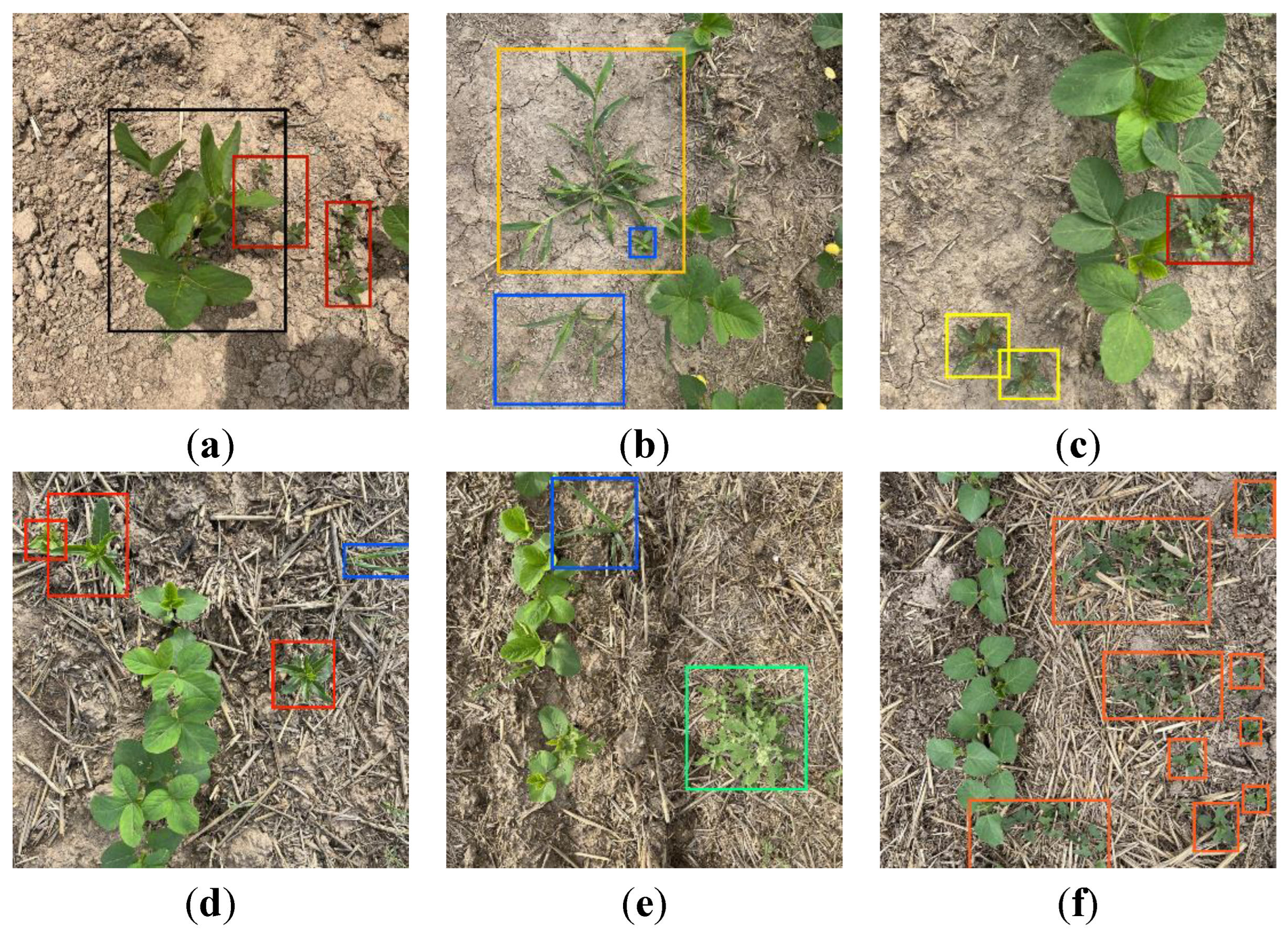
Figure 1. Sample images of different growth states of soybean seedlings and various weeds: (a) Soybean seedlings in the black frame and Purslane in the red frame; (b) Soybean seedlings, the Herb of Common Crabgrass in the light orange frame, and the non-target object in the blue frame; (c) Soybean seedlings, the Copper leaf Herb in the yellow frame, and Purslane; (d) Soybean seedlings, the Spinegreens weed in the red frame, and non-target objects; (e) Soybean seedlings, the Chenopodium album L. in the green frame, and non-target objects; (f) Soybean seedlings and the Calystegia hederacea Wall. in the orange frame.
Preprints 115627 g001
Figure 2. Schematic diagram of translation operation: (a) In the figure, M i n x u l i = 0 , l M a x x l r i = 0 , so horizontal movement is not possible, and the vertical movement range is [ 1073,1929 ] . However, vertical translation is possible, b r = 5 ; (b) In the figure, the horizontal movement range is 1094,686 , horizontal movement is possible, a r = 5 . M i n y u l i = 0 , w M a x y l r i = 0 , so vertical movement is not possible; (c) In the figure, M i n x u l i = 0 , M i n y u l i = 0 , M a x x l r i = 3024 , and M a x y l r i = 3024 , so movement is not possible; (d) In the figure, M i n x u l i = 1137 , M i n y u l i = 833 , M a x x l r i = 1746 , and M a x y l r i = 2664 , the horizontal movement range is [ 1137,1278 ] , a r = 5 . The vertical movement range is [ 833,360 ] . Both horizontal and vertical translations are possible, a r = 5 , b r = 5 .
Preprints 115627 g002
Figure 3. Examples of data enhancement effects: (a) Original image, (b) Right panning, (c) Panning + Vertical flip, (d) Rotate + Horizontal flip, (e) Panning + Vertical flip + Reduction brightness, (f) Rotation + Reduction brightness + Gaussian noise.
Preprints 115627 g003
Figure 4. CSPPC structure module.
Preprints 115627 g004
Figure 5. Ordinary and Ghost convolution modules.
Preprints 115627 g005
Figure 6. Mixed local channel attention mechanism.
Preprints 115627 g006
Figure 8. Schematic diagram of ESWIM working principle.
Preprints 115627 g008
Figure 9. Different positions of the MLCA module: (a) SWIM_S: Output position of the MLCA module at the small target detection layer; (b) SWIM_M: Output position of the MLCA module at the small target detection layer; (c) SWIM: Output position of the MLCA module at the small target detection layer; (d) SWIM_A: Output positions of the MLCA module at three target detection layers.
Preprints 115627 g009
Figure 10. Experimental results of the SWIM model and YOLOv5n model: (a) Evaluation metrics for the validation set and application scenario test set of the SWIM model under different dataset sizes; (b) Evaluation metrics for the validation set and application scenario test set of the YOLOv5n model under different dataset sizes; (c) AP of various weed types in the application scenario test set of the SWIM model under different dataset sizes; (d) AP of various weed types in the application scenario test set of the YOLOv5n model under different dataset sizes.
Preprints 115627 g010aPreprints 115627 g010b
Table 1. Statistics of target data in the 1336 dataset.
Datasets Overall Soybean Weeds machixian matang tiexiancai ciercai li dawanhua
Test set (89) 529 307 222 115 24 21 13 3 46
Valid set (312) 1957 1206 751 367 93 47 75 14 155
Training set (935) 6141 3476 2665 1158 321 146 225 24 470
Dataset (1336) 8627 4989 3638 1640 438 214 313 41 671
Proportion of each target (%) 100 57.83 42.17 19.01 5.08 2.48 3.64 0.48 7.78
Table 2. Experimental Parameters.
Parameters Values
Image size 640×640
Optimizer SGD
Epoch 200
Batch size 16
Learning rate 0.02
Weight decay 0.0005
Momentum 0.937
Table 3. Performance metrics of ablation experimentsts.
Methods Ghost CSPPC mAP@0.5 Parameters/M GFLOPs Model Size/MB
YOLOv5n 90.2 1.77 4.2 3.76
C_YOLOv5n 91.8 1.27 3.0 2.75
G_YOLOv5n 89.1 1.47 3.6 3.21
SWIM_T 88.4 0.97 2.3 2.20
Note:√ Indicates that the baseline network uses this module.
Table 4. Comparison results of different positions of the MLCA module.
Methods mAP@0.5 Parameters/M GFLOPs Model Size/MB
SWIM_S 86.8 0.97 2.7 2.21
SWIM_M 88.1 0.97 2.7 2.21
SWIM 90.3 0.97 2.7 2.21
SWIM_A 88.4 0.97 2.7 2.21
Table 5. Experimental results of augmented partitioning for datasets with different sequencing orders.
Model Datasets Valid mAP@0.5(%) Application Scenario Test mAP@0.5(%)
mAP Soybean AP Weeds AP mAP Soybean AP Weeds AP
SWIM dataset 1 99.5 99.5 99.5 79.7 94.0 77.3
dataset 2 68.8 92.4 64.8 78.0 94.7 75.2
Table 6. Comparison results of the evolutionary experiment.
Models Datasets mAP@0.5(%)
mAP Soybean Seedling AP Weeds AP
SWIM Original Dataset 90.3 95.9 89.4
ESWIM Evolutionary Dataset 90.7 96.7 89.7
Disclaimer/Publisher’s Note: The statements, opinions and data contained in all publications are solely those of the individual author(s) and contributor(s) and not of MDPI and/or the editor(s). MDPI and/or the editor(s) disclaim responsibility for any injury to people or property resulting from any ideas, methods, instructions or products referred to in the content.
Copyright: This open access article is published under a Creative Commons CC BY 4.0 license, which permit the free download, distribution, and reuse, provided that the author and preprint are cited in any reuse.
Prerpints.org logo

Preprints.org is a free preprint server supported by MDPI in Basel, Switzerland.

Subscribe

© 2024 MDPI (Basel, Switzerland) unless otherwise stated