1. Introduction
Alzheimer’s disease (AD) is a neurodegenerative condition, and is one main cause of dementia which is a clinical syndrome. Timely and proactive evaluation is critical to initiate therapy and deliver quality patient care [
1]. According to the Institute for Health Metrics and Evaluation (IHME), the global prevalence of dementia is projected to rise from 57 million cases in 2019 to 153 million by 2050 [
2]. Similarly, the World Health Organization (WHO) predicts that AD will become the sixth leading cause of death by 2050, surpassing cancer, with an estimated 152 million fatalities [
3]. AD is a chronic neurodegenerative disorder that progressively destroys brain cells, leading to memory loss, cognitive impairments, and a decline in the ability to perform daily activities [
4].
The National Institute of Neurological Disorders and Stroke describes AD as a disorder characterized by gradual brain tissue loss, resulting in memory loss, cognitive dysfunction, and behavioral changes. Dementia, caused by brain atrophy, manifests through memory decline and a deterioration in cognitive, social, and behavioral abilities [
5]. Although the precise origins of Alzheimer’s disease are still unclear, it is known that malfunctions in brain disrupt neuronal function, leading to a cascade of harmful effects. Damaged neurons eventually lose connections and die [
6,
7,
8,
9]. AD is a fatal, incurable disease that causes physical, and financial difficulties along with extensive mental suffering throughout the patient’s life [
10,
11]. Currently, no treatments or drugs have been shown to reverse dementia, and the cause of AD is still elusive. Neither are drugs available to slow the progression. Mild cognitive impairment (MCI) considered a preclinical stage of AD, is serving as a transitional phase between normal aging and the onset of AD [
12].
Early identification of AD risk and severity is crucial [
13,
14]. However, neuroimaging and computer-assisted diagnosis often fall short in detecting early stages of AD. Medical diagnosis heavily relies on neuroimaging techniques such as Computer Tomography (CT) scans, Positron Emission Tomography (PET) scans, and particularly Magnetic Resonance Imaging (MRI) scans [
15]. MRI is a reliable, non-invasive technique for examining the human body. The advent of computer-aided diagnosis has spurred significant research in this field [
16,
17].
Various Artificial Intelligence (AI) algorithms have been developed for AD detection and classification. Convolutional Neural Networks (CNN) showed encouraging results, although there remains room for improvement [
18,
19]. Recent advancements include models such as a deep model with slice selection, a hybrid CNN, and a deep CNN with histogram stretching [
20,
21,
22]. Other approaches include CNN models with skull stripping [
23] and pre-processing of slicing samples [
24]. Despite their potential, CNNs’ inherent black-box nature often biases these deep models towards classification.
Automated neuro-image segmentation methods and programs have also been developed, as highlighted in the AD literature [
25]. Notable applications include Neuro-Imaging Pre-processing Fusion [
26] and Vol-Brain [
27]. While these programs aid in neuro-image segmentation, there has been limited research on visualizing classification steps using CNN layers. Each convolution layer’s feature map reveals different filters applied to the image, indicating the types of filters the model employs to extract features [
28]. This method aligns with the Grad-CAM [
29] heat map, which uses a gradient-based localization map to display class activation.
The method uses a deep CNN model with standard layers to get good classification results. The proposed method uses CNN deep layers to visualize the classification process and get the state-of-the-art (SOTA) classification model for early AD detection. The study’s key findings:
The proposed network is a generalized model that is better than other models and can easily find several AD classes. It was trained with minimum parameters and had a low computational cost.
Due to an inequitable distribution of Alzheimer’s data, the accuracy of prior approaches is diminished in [
22,
23,
25]. To address more issues in the Alzheimer’s data set, the oversampling technique SMOTE is used to interpolate images to create more representative samples of each class.
The intensity of the Bio-AD model’s heat map, which was made using the Grad-CAM method to map damaged brain regions, showed how bad each stage of Alzheimer’s disease was.
The proposed model is thoroughly compared to various alternative methods using several evaluation measures such as Accuracy, AUC, Precision, Recall, F1-score, and the number of trainable parameters. In comparison with other cutting-edge models, our technique outperforms.
This section of the paper is structured as follows: A summary of the research is pertinent to this discussion can be found in
Section 2. Methodology, the Bio-AD model for AD classification details, and a description of data collection and model components are presented and described in
Section 3. The Bio-AD visualization approach and evaluation are in
Section 4, the limitations of the proposed study with raised concerns are provided in
Section 5, and the study concludes with a discussion of potential next steps in
Section 6.
2. Related Work
Collecting medical datasets is inherently challenging due to privacy concerns and the sensitivity of patient information. This complicates the task of medical image categorization, as sharing these datasets is often restricted [
30]. Organizations for example Alzheimer’s Disease Neuroimaging Initiative (ADNI) [
31] and the Open Access Series of Imaging Studies (OASIS) [35] facilitate access to these datasets under strict conditions. Researchers must apply for access and comply with restrictions on data usage, which adds another layer of complexity.
Medical datasets often exhibit significant class imbalance, with an unequal number of healthy and diseased patients, further complicating the development of robust models [36,37,38,39]. Addressing this imbalance is a significant challenge that researchers have tackled using various techniques [40,41,42,43].
In a recent study, a CNN model was developed using the OASIS dataset, which includes 416 3D samples. The model consisted of convolutional layers, batch normalization, pooling layers, and an SGD optimizer [44]. The model’s performance was benchmarked against pretrained models including InceptionV4 [45] and ResNet, demonstrating competitive accuracy.
A cost-sensitive training technique was proposed in [46] to address the dataset imbalance issue. This method employed a cost matrix to adjust the output layer, giving more weight to underrepresented classes, resulting in a 75% accuracy rate. Similarly, Hussain et al. used the OASIS dataset and a 12-layer CNN architecture incorporating Leaky ReLU to prevent the gradient vanishing problem [47]. Their model achieved 97.75% overall accuracy and a comparison was made against pretrained models like InceptionV3, Xception [48], MobileNet-V2 [49], and VGG-19 [
25].
Sugnathe et al. [
14] implemented a hybrid architecture combining ResNetV2 and InceptionV4 using the Kaggle dataset. The ResNetV2 model incorporated residual connections to the pre-trained InceptionV4 model [43], achieving a maximum accuracy of 79.12% with various learning rates and optimizers. Pradhan et al. [35] conducted a comparative evaluation using VGG-19 and DenseNet-169 due to their capability to handle vanishing gradients and train on numerous classes with high accuracy. They utilized the Kaggle dataset augmented with the Image Data Generator (IDG), resulting in accuracy rates of 88% and 87%, respectively. In another recent study, Bettini et al. [37] developed a five-layer CNN model using the OASIS-3 dataset to categorize early stages of Alzheimer’s disease. This model demonstrated significant potential in distinguishing between different stages of the disease [50].
More recently, novel techniques such as transfer learning and ensemble methods have been explored. For instance, Zhang et al. [65] proposed an ensemble of CNNs that achieved an accuracy of 93.5% on the ADNI dataset by combining multiple models’ outputs to improve robustness. Similarly, Liu et al. [66] applied transfer learning using pre-trained models on a large-scale brain MRI dataset, achieving improved performance with reduced training times. Additionally, the use of advanced preprocessing techniques has shown promise. Patel et al. [67] demonstrated that incorporating sophisticated image preprocessing methods could significantly enhance model performance, leading to more accurate and reliable diagnostics.
Not all features extracted by deep models are useful for accurately predicting the class of a sample. Some features prevent a model from producing the anticipated outcomes [66,67]. El-Aal et al. [
29] addressed this issue with deep models and offered a novel method for choosing particular features from the feature map of deep models, enhancing classification performance, and shortening model training time. The Rival Genetic Algorithm (RGA) [68] and Probability Binary Particle Swarm Optimization (PBPSO) cite RN52 methods were employed for feature extraction, while ResNet101 and DenseNet201 were used for feature selection. An independently developed classification model was fed the chosen and control features with PBPSO, ResNet101, and DenseNet201 produced the most outstanding results, with accuracy rates of 87.3 and 94.8 percent, respectively. Grad-CAM, a class activation heat-map approach that utilizes gradient data in its computation along with heat (density) map to assist in comprehending the operation of a deep learning model, was used by Raju et al. [70]. To accomplish this, they decided to use transfer learning to train a neural network, and they changed the VGG-16 by including an auxiliary dense layer towards the network’s last part. Fastai at el. [71] leverages Grad-CAM to emphasize the brain regions in MRI scans that the previous model selects for its predictions, which improves the model’s performance. The classification outcomes were further enhanced using the loss function Stochastic Gradient Descent (SGD) in conjunction with the Nesterov intensity [72]. As a result, the model reached 97.89% test accuracy.
The majority of researchers have not produced particularly impressive classification results, and there is always room for improvement in DL. Their practices are limited by various factors, as they did not fully consider the inherent challenges of medical imaging datasets and certain deep learning models.
Table 1 compares and contrasts the most recent classification models for Alzheimer’s disease. We are attempting to combine established deep and transfer learning models with cutting-edge methodologies to attain exceptional accuracy outcomes of over 90%.
3. The Bio-AD Model for Diagnosis of Alzheimer’s Disease
Today, image processing is utilized in almost all aspects of treatment. During the diagnostic stage, doctors can examine the human body’s internal organs without needing surgery. A person cannot accurately interpret medical scans as a computer can and draw the necessary conclusions from them. On the other hand, it can take a whole team of medical professionals days to reach the same decision. A system that has been taught to analyze medical images may produce reliable results in a flash. Algorithms for computer vision and image processing are crucial components of contemporary healthcare systems. One cannot express how important this is. One of the diseases with the fastest rate of growth on a global scale is AD. A few researchers have improved their outcomes by using data augmentation approaches. In contrast, the essential issue of data set imbalance has not been acknowledged in any of the examined research studies involving the classification of Alzheimer’s disease. Due to inadequate model training, some researchers were unable to obtain noteworthy results. It has been noted that research publications tend to concentrate on developing fresh methods for categorizing biomedical diagnosis.
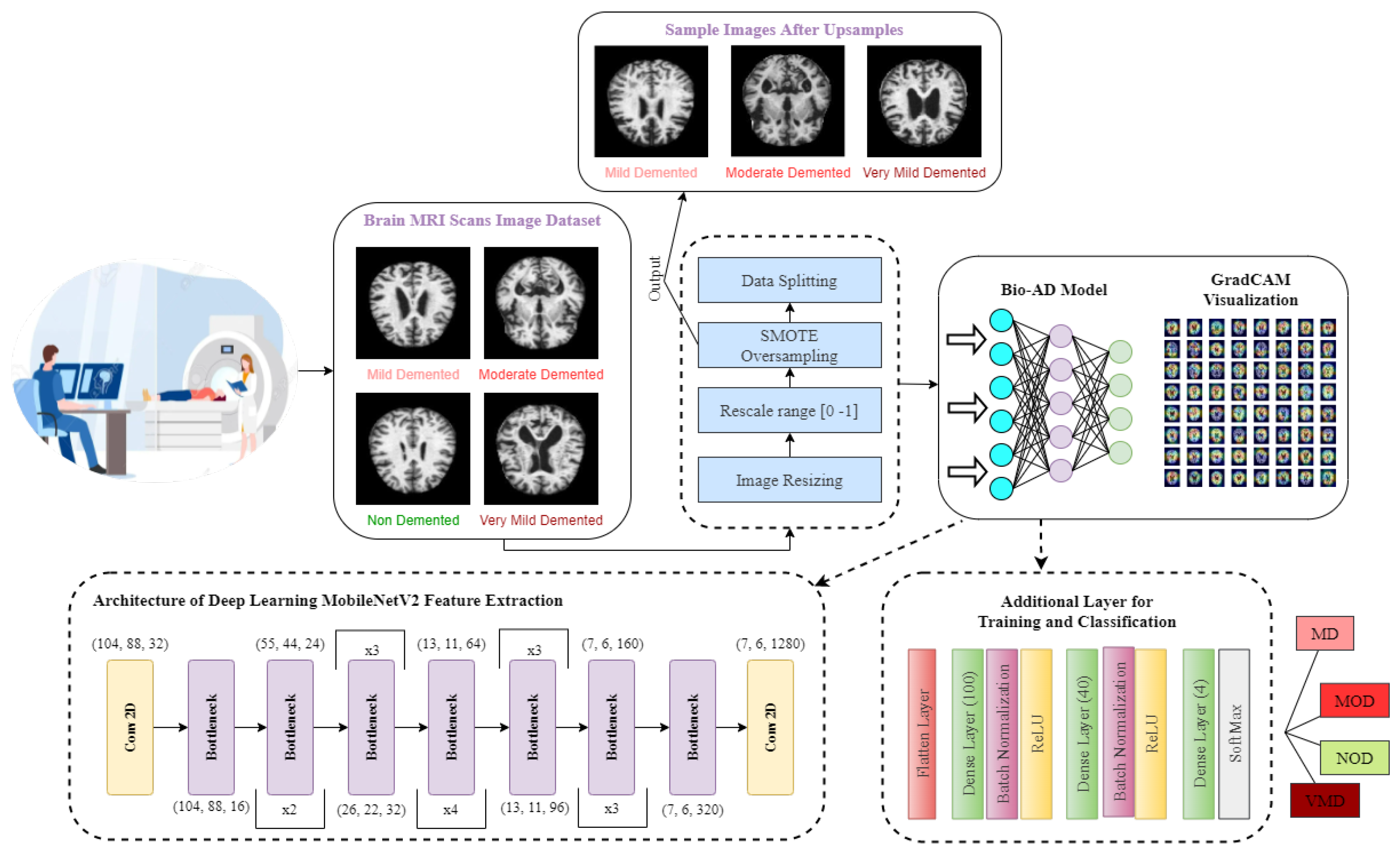
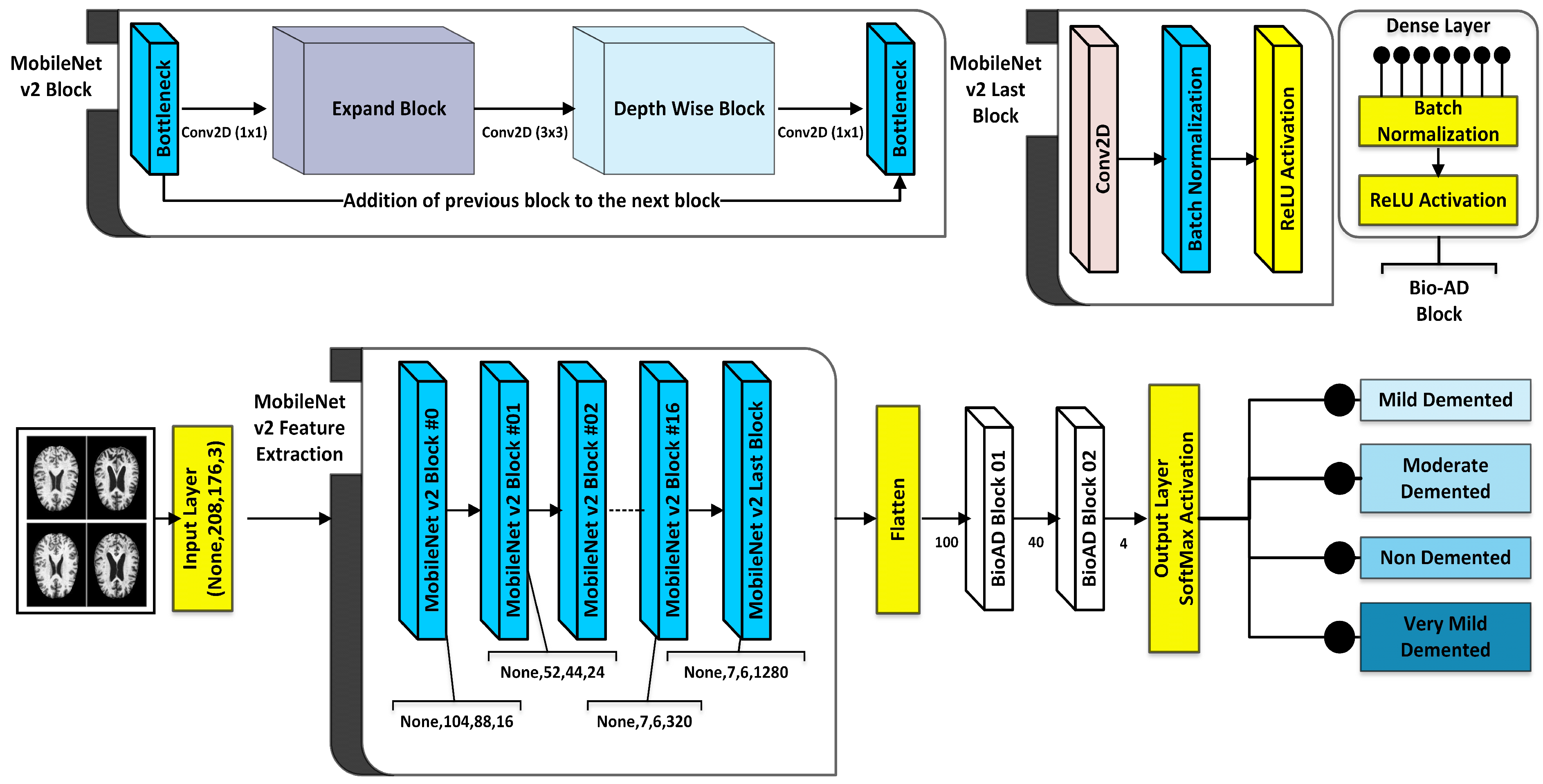
As part of the Bio-AD model, the input data set is normalized, and the critical conversion of categorical features to be given to the model through one-hot encoder is carried out. Unbalanced classes issue is addressed using the Synthetic Minority Oversampling Technique (SMOTE) to oversample the minority classes. The dataset is then split into 80%, 10%, and 10% portions for training, validation and testing, respectively. The MobileNet-V2 architecture is subsequently used for feature engineering. In order to develop our model, Bio-AD, for useful and accurate training, we again employed transfer learning with MobileNet-V2 but excluded the top portion and added several layers in the next MobileNet-V2 model, as shown in
Figure 1. For the model’s robustness in AD classification, the training parameters are decreased as compared to [29,35,37,73,74]. Grad-CAM heat-map technique is used for showing class activation map and draw attention to the features of an image sample that help classify it.
3.1. Alzheimer’s Disease Data Set Description
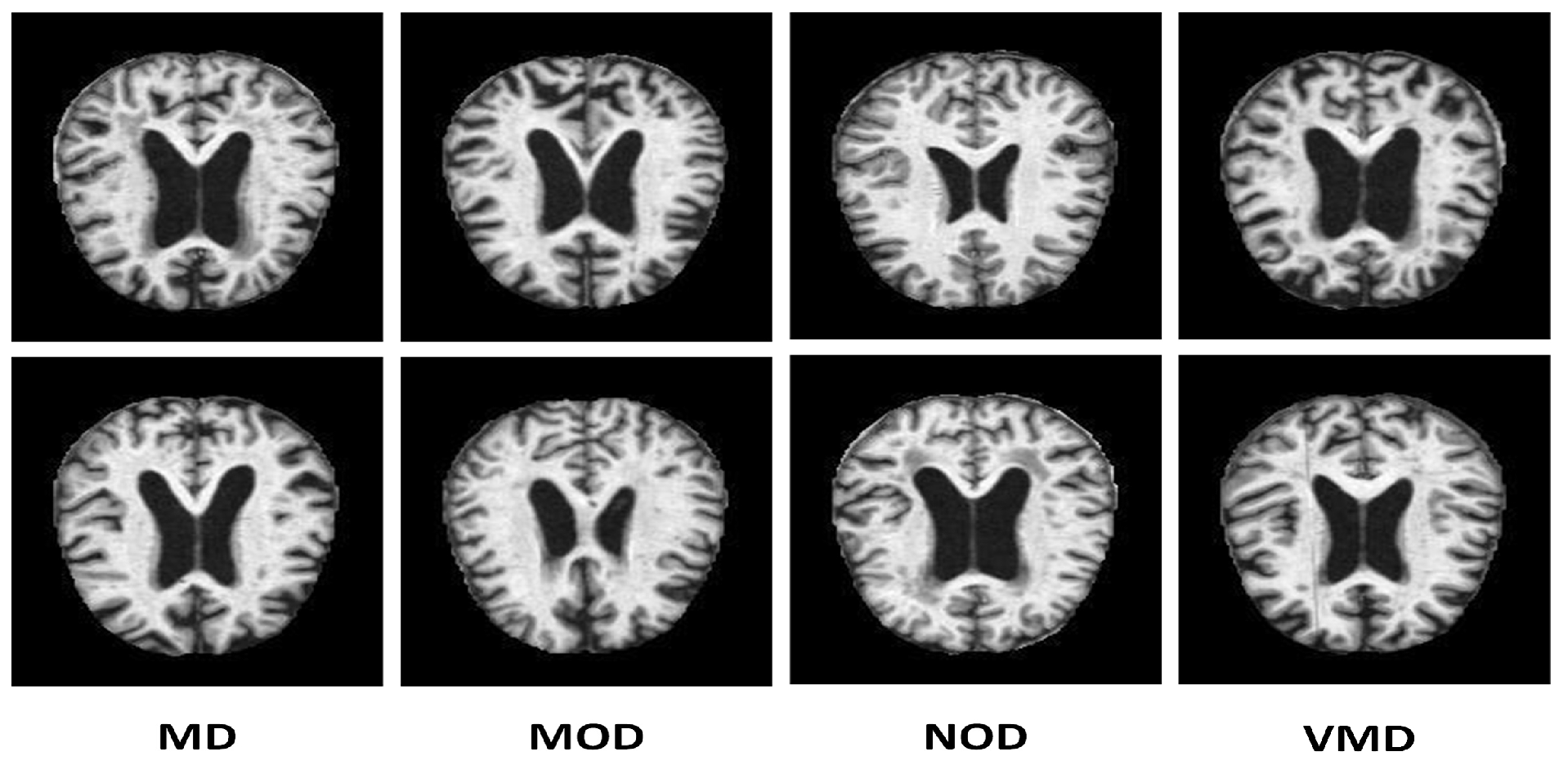
Many online data sets can be used to categorize AD properly. Organizations like ADNI and OASIS are working hard to ensure that researchers and educators have access to these data sets. However, the samples in both of these datasets are presented as three-dimensional graphics, and the datasets themselves are massive. In perspective, the OASIS dataset occupies space of about 18 TB, while the size of ADNI datset is about 450 GB. Kaggle data collection was used for this study since it contains only samples of anonymized MRI scan images and their associated classifications. This dataset is multiclass since it has four categories and many perspectives. A typical NOD group with three other groups representing the premature stages of Alzheimer’s disease (MD, MOD, and VMD) is shown in
Figure 2.
As stated in the Kaggle’s dataset description, every representative sample has been manually verified by the user. Furthermore, the parts have already been cleaned up, that is, downsized and arranged, and the scale of the data set is manageable. The dataset shows precision of 2 decimal points [76]. Several other studies used this dataset with this precision for analysis [77]. This data collection is utilized in our study based on these variables. There are 6400 total samples in the data set. The examples are separate 176 x 208-pixel RGB three-channel images from four different classes. The NOD class consists of 3200 pieces. There are 896, 64, and 2240 photos in the last three classes, MD, MOD, and VMD, respectively. The imbalance in this data collection, which is explained in
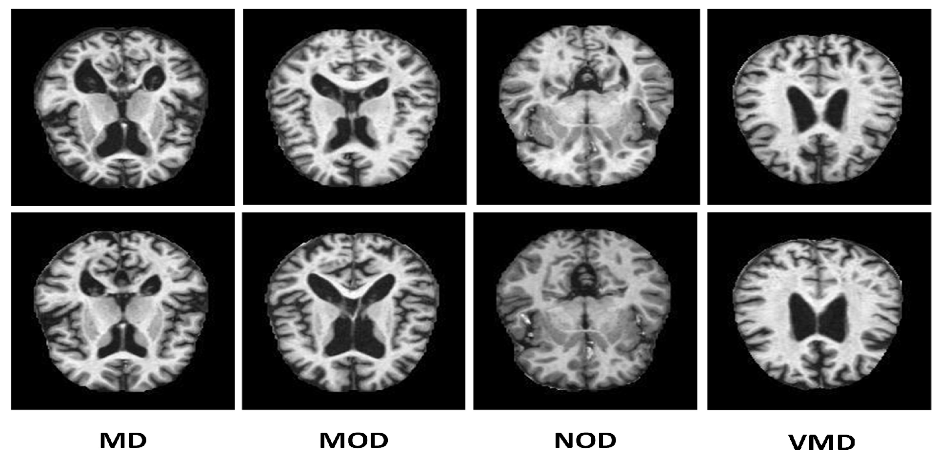
Table 2 is its only drawback. To address this problem, we used SMOTE to produce fictitious data, for each imbalance class with regards to the balanced type as displayed in
Figure 2. Splitting of the dataset into training, validation, and test sets was made with proportions of 80%, 10%, and 10%, respectively.
3.2. Balancing the Data Set through SMOTE
We have employed the oversampling technique to handle the data set imbalance problem. Oversampling algorithms generate new samples based on the original instances. SMOTE [75] algorithm constructs new pieces by interpolating even the class samples in the data set. MD, MOD, NOD, and VMD classes initially have 896, 64, 3200, and 2240 images, as discussed in
Table 3. SMOTE employs the Nearest Neighbor approach for balancing the data set and to interpolate additional imitation examples for the minority classes depicted in
Figure 3.
3.3. The MobileNet-V2
A lightweight deep neural network model, MobileNet-V2, offers superior classification accuracy with fewer parameters, making it highly suitable for image categorization and mobile vision applications. Unlike traditional models that combine and attend to convolutions across all color channels, MobileNet-V2 employs depth-wise separable convolutions in each color channel. This depth-wise separability divides the convolutions into two layers: a filtering layer and a connecting layer, effectively reducing computation and model size. This architecture is particularly advantageous for embedded systems due to its minimal processing power requirements and high classification potential, especially in the medical field. MobileNet-V2 enables the creation of artificially intelligent medical devices that are resource-efficient, quick to respond, and highly accurate. The model’s architecture is thus ideal for embedded vision applications. Additionally, MobileNet-V2 incorporates two global hyperparameters that balance accuracy and latency, providing a detailed parameter description and facilitating an in-depth examination of its architecture. This balance makes MobileNet-V2 a versatile and powerful tool for applications requiring efficient and accurate image processing.
3.4. The Proposed Bio-AD Network Architecture
CNN, which relies on the biological characteristics of the cerebrum of human beings, is particularly useful for object identification, image classification, and image segmentation in computer vision applications. They are chosen because they are translation-invariant [73,74]. To conduct precise AD categorization, a unique CNN model is created from scratch in this study. Our model consists of MobileNet-V2 (
Conv2D, BatchNormalization, Activation) layers and Dense layers with SoftMax activation faction.
Figure 4 contains general information regarding the Bio-AD model and depicts the Bio-AD architecture for the Alzheimer’s classification as described in
Table 4.
3.4.1. Flatten Layer
Between the dense and convolution layers is a flatten layer. Dense layers need data in a 1-Dimensional format, whereas convolution layers accept tensor data types as input. The feature map is vectorized using a flattening layer and then feeding it to dense layers.
3.5. Bio-AD Block
The suggested architecture consists of two Bio-AD blocks, each of which comprises a few levels. The next subsection discusses the specifics of each layer.
3.5.1. Dense Layer
Dense Layer often referred to as "fully connected layer", generates a single vector as its output. That vector takes its attributes from the input vector. These layers are responsible for picture recognition and the assignment of a class label. The model acquires knowledge by using the back-propagation approach in entirely linked layers. The count of model’s trainable parameters depends on values utilized in fully connected layers. After several layers, the SoftMax function is applied, and the number of neurons in the network is configured to match the number of classes as described in [69]. In multi-class classification method, One-hot method is used for encoding the labels, and the loss term only includes instances of the positive type.
3.5.2. Batch Normalization
The batch Normalization algorithm normalizes the activation vectors from convolutions layers. It is precious when training is performed in batches. It standardizes the values, resulting in faster and more regular movement of the model.
3.5.3. Activation Functions
To determine whether a perceptron’s output should be sent to the following layer, activation functions use mathematical calculations. In a nutshell, in neural networks, they turn on and off the nodes. The node is activated in last layer using the activation function. The last layer then returns its label and assigns it to the picture that has been subjected to model processing. There are a variety of activation functions; because ReLU’s computations are quick and easy, we employed it in hidden layers.
SoftMax, an activation function that is dependent on probability, is utilized in the output layer of the proposed model, which manages the multi-class classification.
4. Analysis and Evaluation of the Bio-AD Model
A Computer with dual 3.0 GHz Intel Xeon 2687W v4 CPUs, 64 GB of RAM, and a 5 GB NVIDIA P2000 GPU was used for the tests. The model evaluation was done using a test set that was created by splitting the dataset prior to training. Its robustness was confirmed through the use of multiple metrics.
How well these results are comprehended collectively determines how successfully a model is trained. In the following equations, the terms TP, TN, FN, and FP stand for True Positive, True Negative, False Negative, and False Positive values accordingly.
4.1. Accuracy
Accuracy is the proportion of actual predictions that were correctly identified, as calculated by the following formulas.
4.2. Precision
Precision measures the proportion of true positive predictions among all positive predictions. The model evaluation is carried out through the test set created from splitting. The precision is given by expression as follows:
4.3. Recall
True positive rate and sensitivity score are other names for recall. It involves evaluating the right positive predictions against the total number of real correct true positives. The recall is calculated using the subsequent equation:
4.4. F1-Score
The best case scenario for a model is one that has precision and recall values of 1.0. The F1-score is the harmonic mean of recall and precision. It is distinctive due to its graphical representation, where each category label is represented by a distinct feature line. The following equation is used to calculate the F1 score:
4.5. Receiver Operating Characteristics (ROC) Curve
The Receiver Operating Characteristics (ROC) curve provides an easy-to-understand and visually appealing illustration of the probable link between sensitivity and specificity for each conceivable cutoff for a set of tests. The ROC Curve graph is presented here where specificity aid is at x-axis and sensitivity is at y-axis. The following equations can be applied in order to calculate the 1-specificity, which is also referred to as the false positive rate (FPR), and the sensitivity, which is also referred to as the true positive rate (TPR):
4.6. Confusion Matrix
To evaluate and determine various categorization model metrics, a confusion matrix is employed. It offers a breakdown of the total number of predictions a model made throughout the training or testing phase.
4.7. Loss Function
Loss functions computes the difference between expected and actual values. A categorical cross-entropy loss method was employed for this study.
4.8. Bio-AD Model Self-Comparison Using ROC
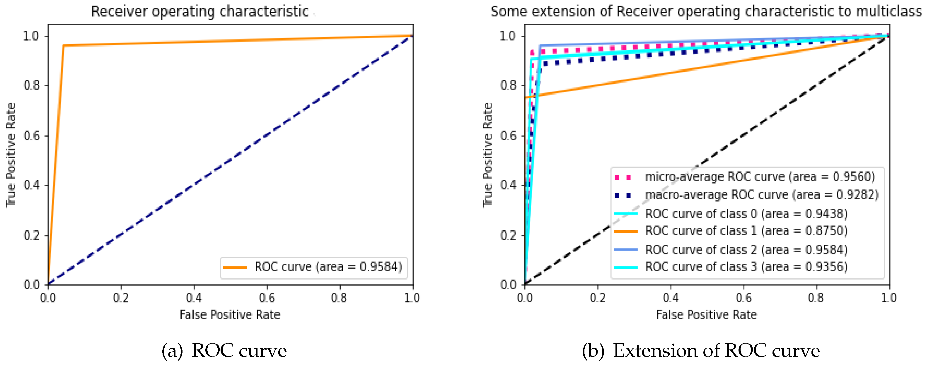
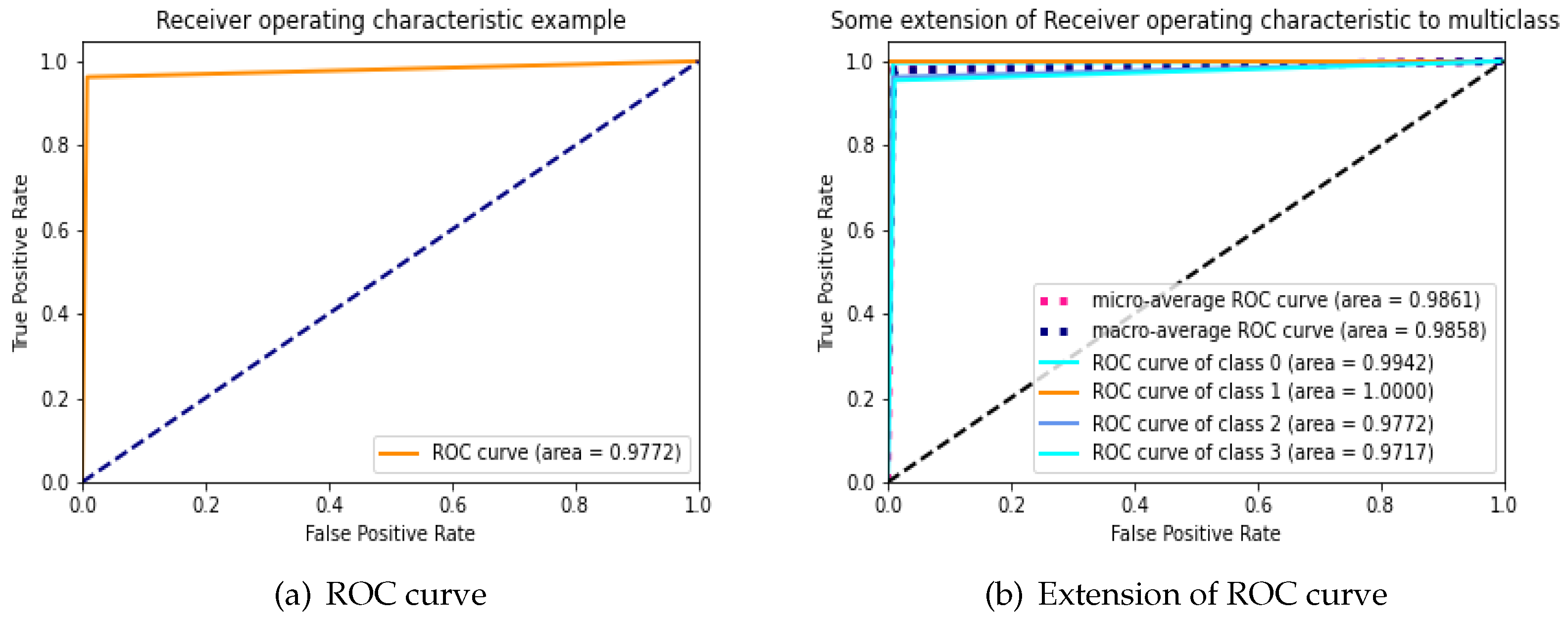
During an analysis of the performance of clinical testing, the ROC curve is specifically used to investigate whether the classifier’s accuracy for binary or multi-class classification can be assessed with reliability. ROC curve’s area under the under (AUC) is used to determine whether or not a classifier is effective; typically, a greater AUC suggests that the classifier is more valuable. We examine the applicability and accuracy of our proposed Bio-AD model by applying it to the AD data set, both with and without SMOTE, and utilizing the ROC curve and extension of the ROC for each class on its own. The AUC values of the proposed model are 97.72% and 95.84% with and without the use of SMOTE, respectively, as shown in
Figure 5a and
Figure 6b. We are able to observe that after employing the SMOTE technique to bring the AD data set into balance, the AUC went from 95.84% to 97.72%, which is a considerable change. The area under the curve (AUC) for classes 0 (MD), 1 (MOD), 2 (NOD), and 3 (VMD) without balancing the data set is 94.38%, 87.50%, 95.84%, and 93.56%, respectively as shown in
Figure 5b. These increases in AUC prove that the SMOTE method and feature selection used in the Bio-AD model is correct.
4.9. Comparison of Accuracy with Other Models Both with and without SMOTE
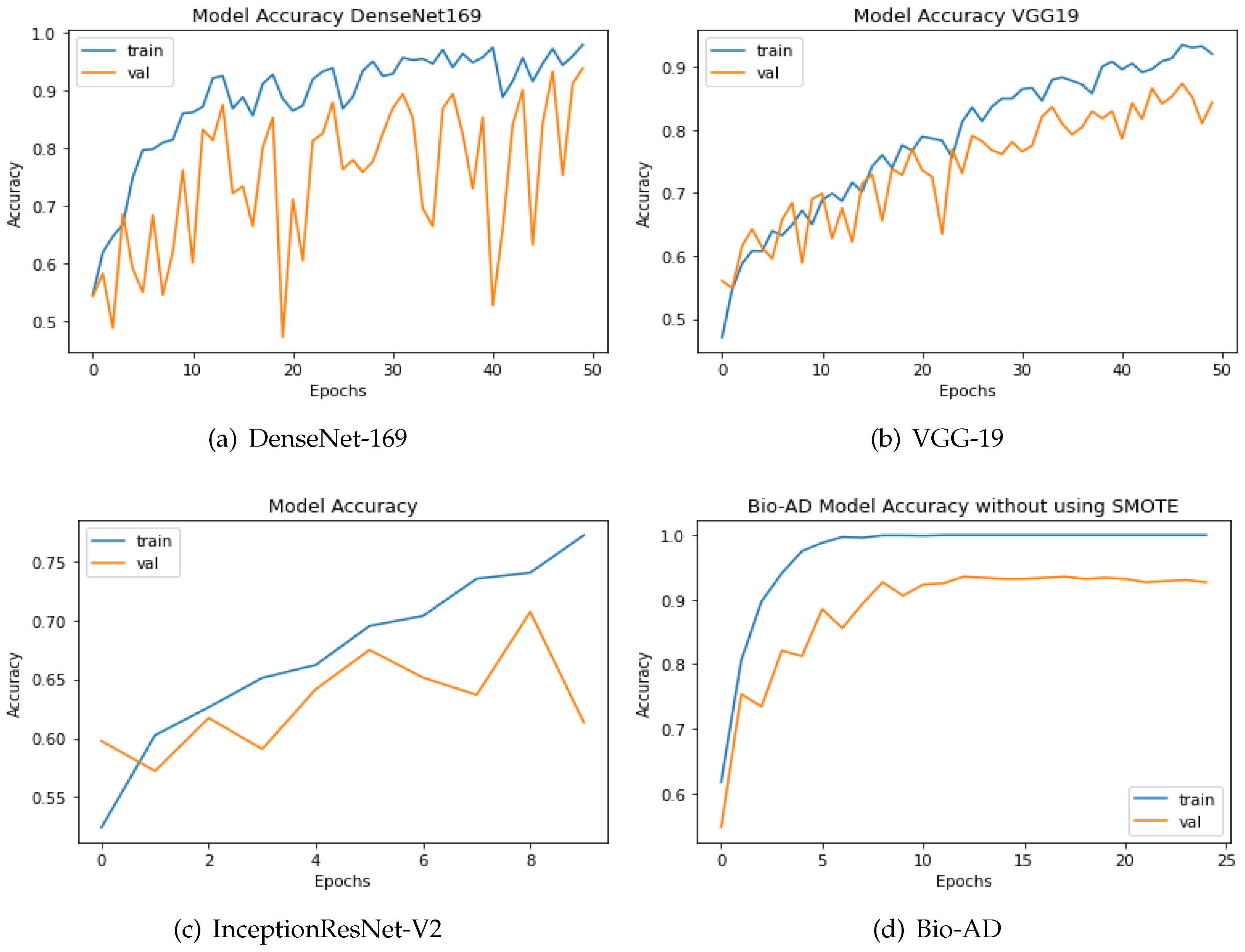
The SMOTE technique is applied to the dataset to boost the quantity of images in underrepresented classes. The number of samples was increased to 12800 from 6400 originally, or 3200 identical images, for each class. The two strategies are compared using the up-sampling technique SMOTE. Both models have a similar design incorporating fully connected dense layers for training, a pre-trained model, and MobileNet-V2 for feature extraction. The same AD dataset was utilized in our research, both before and after SMOTE balancing, to evaluate the performance of our newly proposed models. The results are shown in
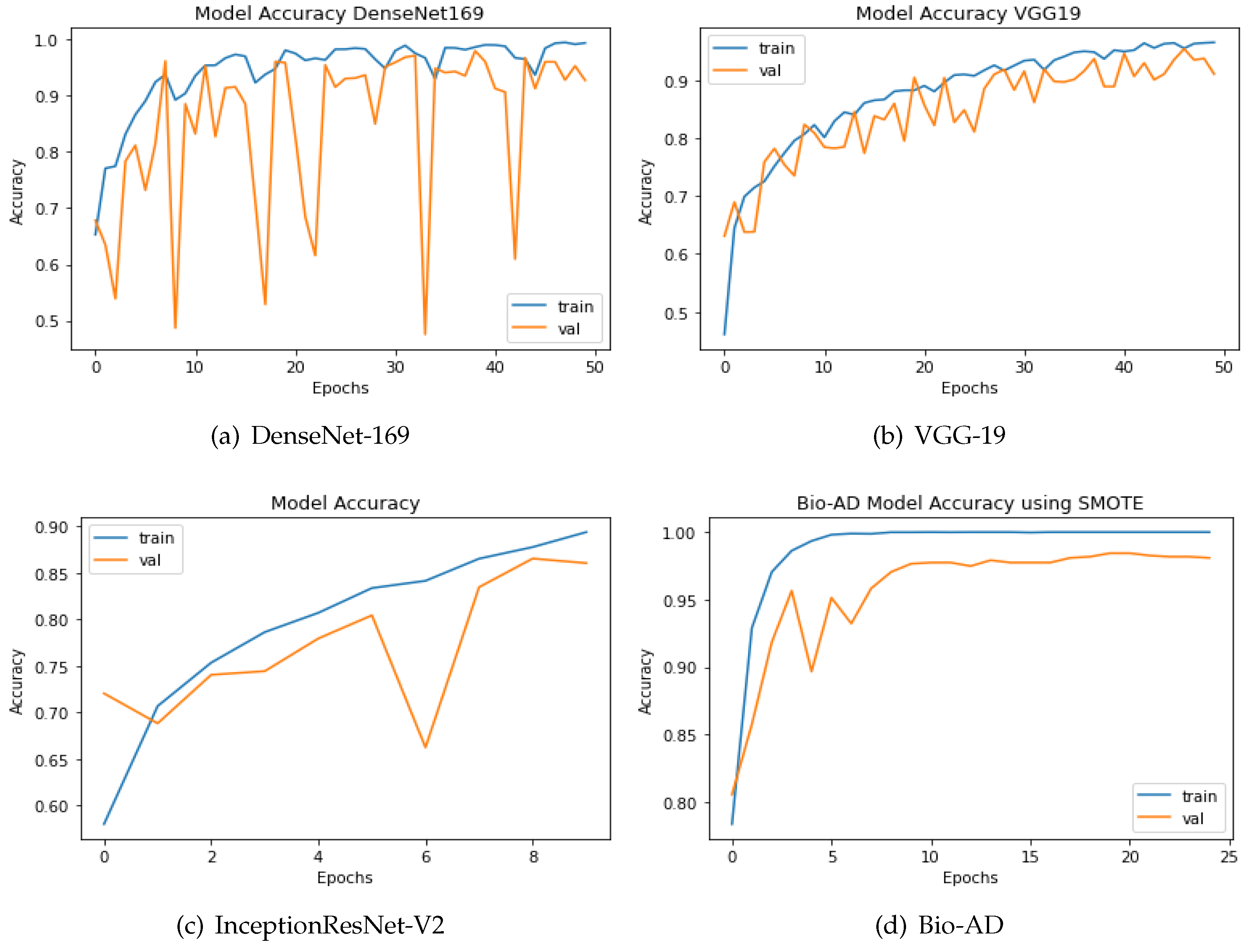
Figure 7. Using an unbalanced AD data set, the proposed Bio-AD model, DenseNet-169, VGG-19, and InceptionResNet-V2 achieved accuracies of 93.40%, 92.72%, 84.38%, and 61.33%, respectively. Using the balanced AD dataset illustrated in
Figure 7, all models, including Bio-AD, DenseNet-169, VGG-19, and InceptionResNet-V2, achieved accuracy rates of 97.92%, 93.75%, 91.02%, and 86.04%, respectively. All models were tested using the balanced AD dataset illustrated in the following figure.
Figure 7.
Accuracy of DenseNet, VGG-19, InceptionResNet-V2 and Bio-AD without SMOTE durint the training process.
Figure 7.
Accuracy of DenseNet, VGG-19, InceptionResNet-V2 and Bio-AD without SMOTE durint the training process.
Figure 8.
Accuracy of DenseNet, InceptionResNet-V2, VGG-19 and Bio-AD with SMOTE during the training process.
Figure 8.
Accuracy of DenseNet, InceptionResNet-V2, VGG-19 and Bio-AD with SMOTE during the training process.
4.10. Comparing the Proposed Models to Other Hybrid Models Using the AUC Metric
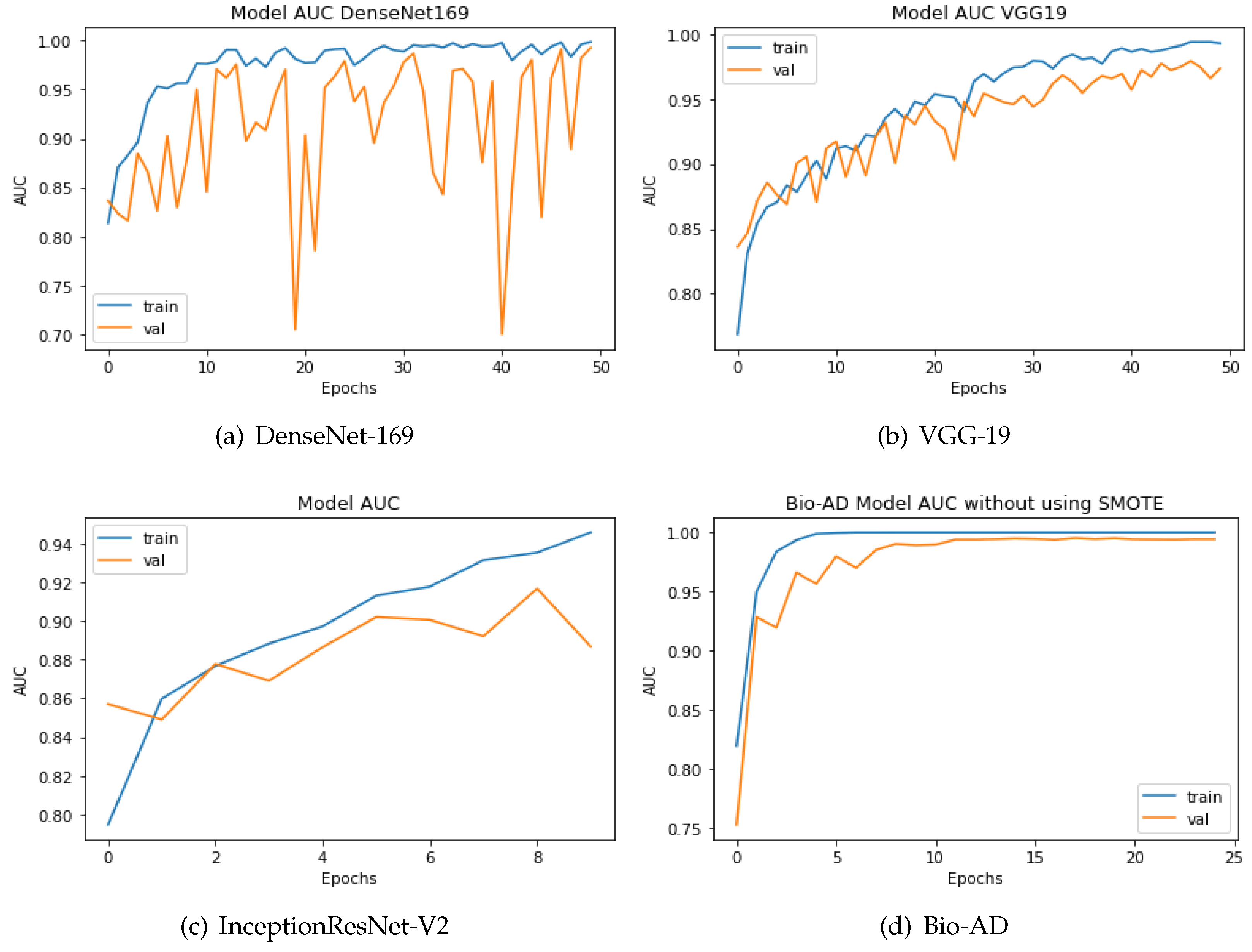
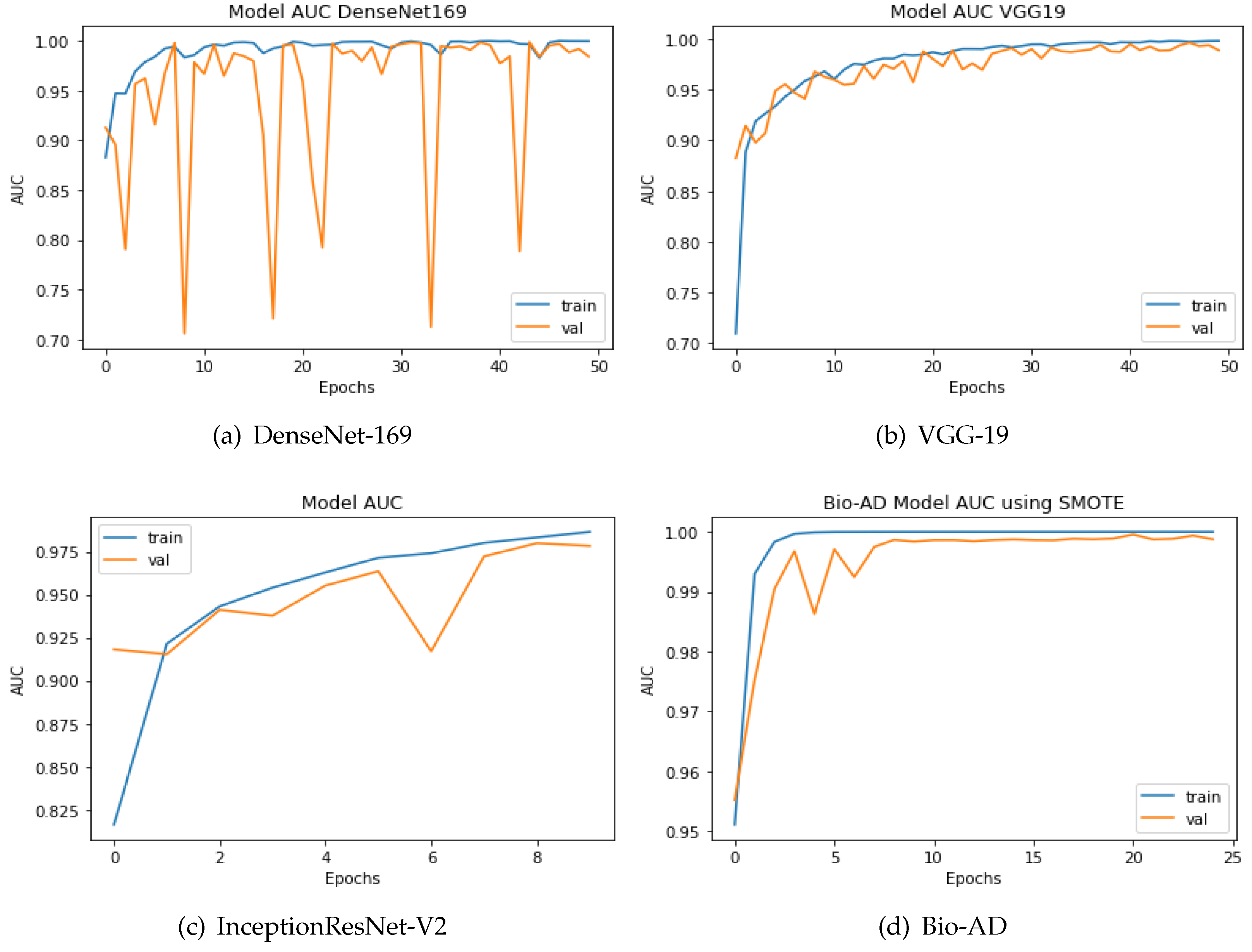
To categorize the early phases of Alzheimer’s disease, various deep models have been developed. Some were conventional CNN models, while the rest included deep architectures that had already been trained. As explained in the previous section, the proposed model is a hybrid architecture of Mobile-Net V2 and a deep neural network based on CNN, Bio-AD network made up of several Bio-AD blocks. Using cutting-edge classification models like InceptionResNet-V2, VGG-19, and DenseNet-169, we also developed other models. We used the AD dataset both before and after SMOTE balancing to compare our proposed and recently developed transfer learning models, such as DenseNet-169, VGG-19, and InceptionResNet-V2. The system yields impressive results with the SMOTE technique for the proposed model. The proposed model along with the other models, is depicted in in Figure 9. The proposed Bio-AD model, DenseNet-169, VGG-19, and InceptionResNet-V2 achieved AUC of 99.24%, 98.40%, 97.36%, 88.67%, respectively using an imbalanced AD data set as shown in Figure 10. All models, like Bio-AD, DenseNet-169, VGG-19, and InceptionResNet-V2 achieved AUCs of 99.87%, 99.25%, 98.89%, 97.83%, respectively using the balanced AD data set.
Figure 9.
Training process AUC of DenseNet, VGG-19, InceptionResNet-V2 and Bio-AD without SMOTE.
Figure 9.
Training process AUC of DenseNet, VGG-19, InceptionResNet-V2 and Bio-AD without SMOTE.
Figure 10.
AUC of the DenseNet, InceptionResNet-V2, VGG-19, and Bio-AD training processes with SMOTE.
Figure 10.
AUC of the DenseNet, InceptionResNet-V2, VGG-19, and Bio-AD training processes with SMOTE.
4.11. Loss Assessment of Bio-AD in Relation to Recent Models
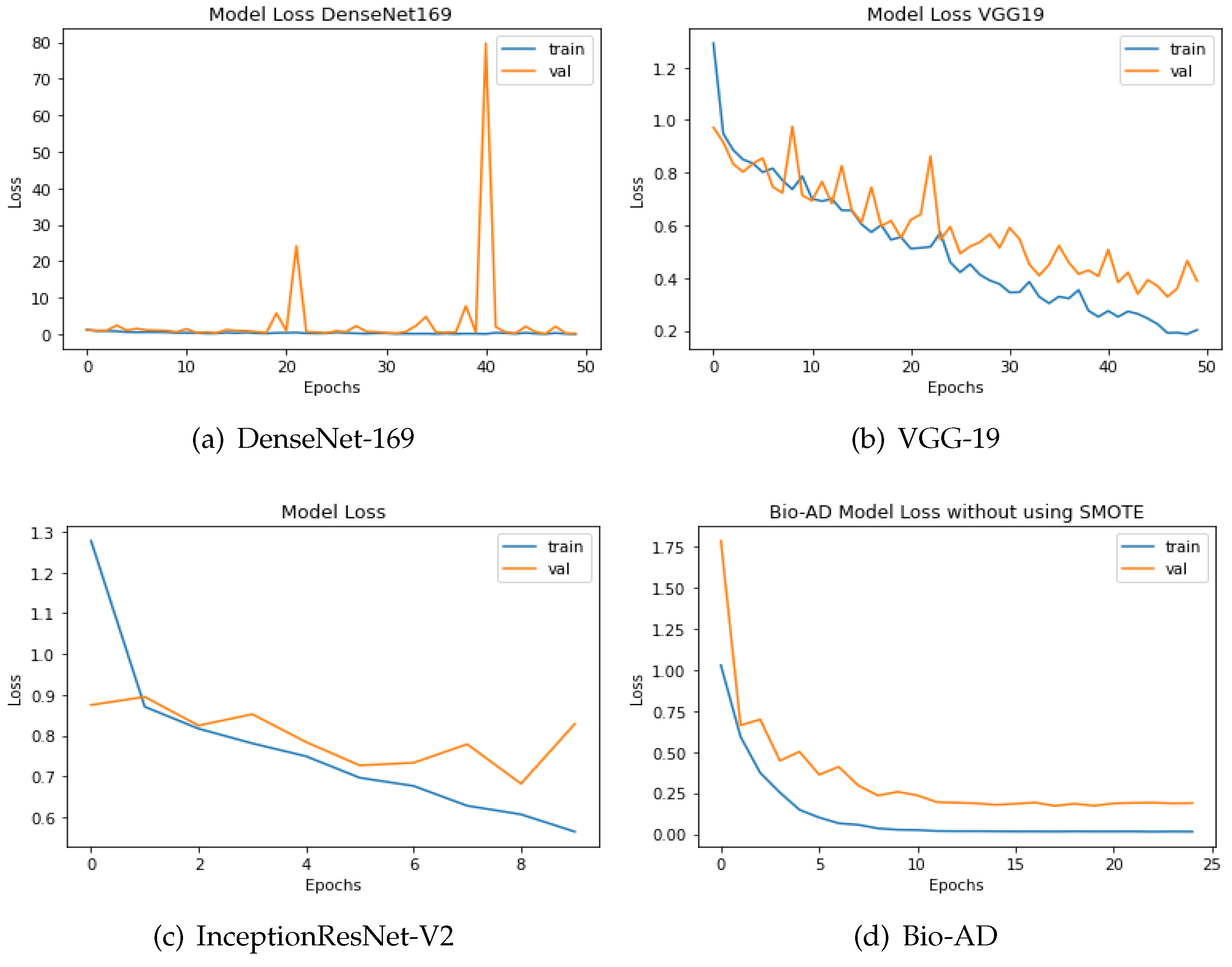
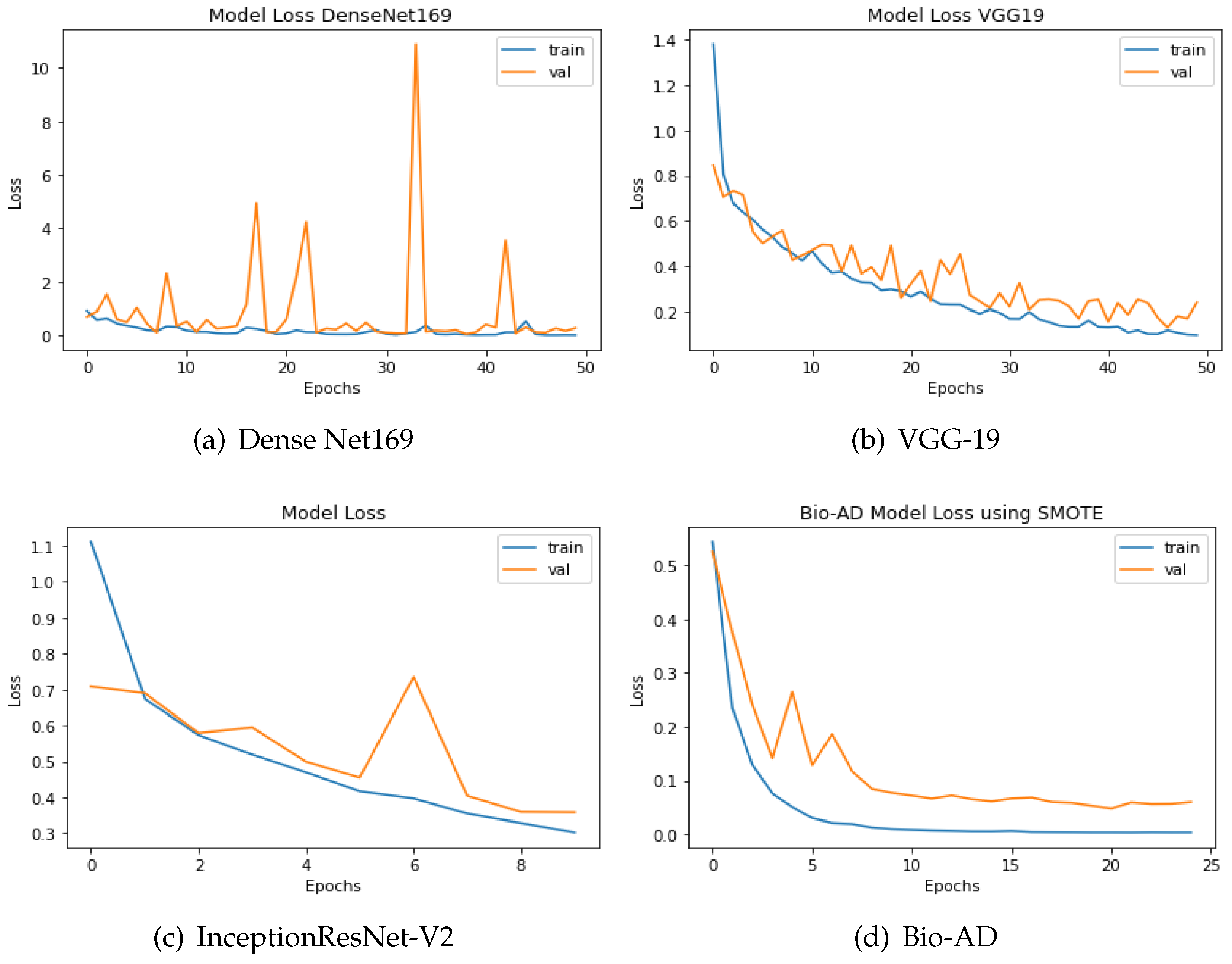
The discrepancy between the predicted and actual values is computed using loss functions. In this study, categorical cross-entropy technique was used for loss calculation. Optimization functions, also known as backpropagation algorithms, adjust the weights and biases of layers based on the magnitude of the loss. The design of both models, which includes a pre-trained model, MobileNet-V2 for feature extraction, and fully connected dense layers for training, is what unites them. Outstanding results are delivered by the model without SMOTE, providing 93.40% accuracy, AUC of 99.24%, and 90.84% percentage value of F1-score. The training accuracy achieved 99.99% for the best-proposed model, 97.92% accuracy for the validation, 99.87% AUC, and F1 score of 97.87%. The efficiency of the two approaches can also be comprehended by the difference in loss values being 0.1955 without SMOTE and merely 0.0646 with SMOTE, as shown in Figure 11 and Figure 12. The loss values for the dataset without SMOTE and with SMOTE are as follows: InceptionResNet-V2 has 0.8286 and 0.3587; DenseNet-169 has 0.2825 and 0.1923; VGG-19 has 0.3890 and 0.2407; and the Bio-AD model has 0.1955 and 0.0646 respectively.
Figure 11.
The loss calculation of DenseNet-169, VGG-19,InceptionResNet-V2 and Bio-AD without SMOTE.
Figure 11.
The loss calculation of DenseNet-169, VGG-19,InceptionResNet-V2 and Bio-AD without SMOTE.
Figure 12.
DenseNet-169, InceptionResNet-V2, VGG-19, and the Bio-AD model with SMOTE for loss assessment.
Figure 12.
DenseNet-169, InceptionResNet-V2, VGG-19, and the Bio-AD model with SMOTE for loss assessment.
4.12. Classification Report of Bio-AD and Other Deep Models
The performance of the models that were constructed without making use of data augmentation or addressing difficulties caused by an imbalance in the data is limited. They also have a high over-fitting problem as a result of the aforementioned issue.
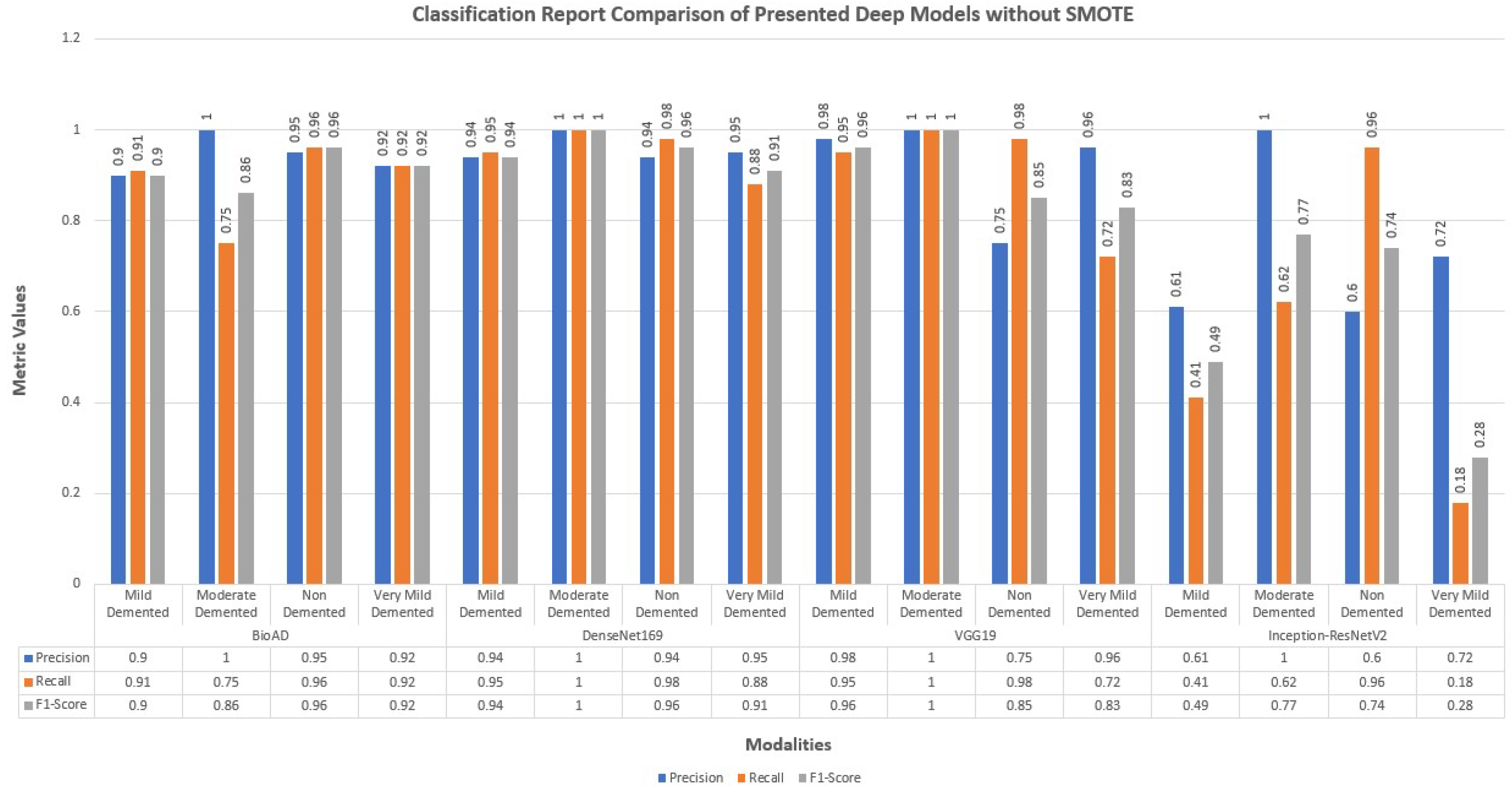
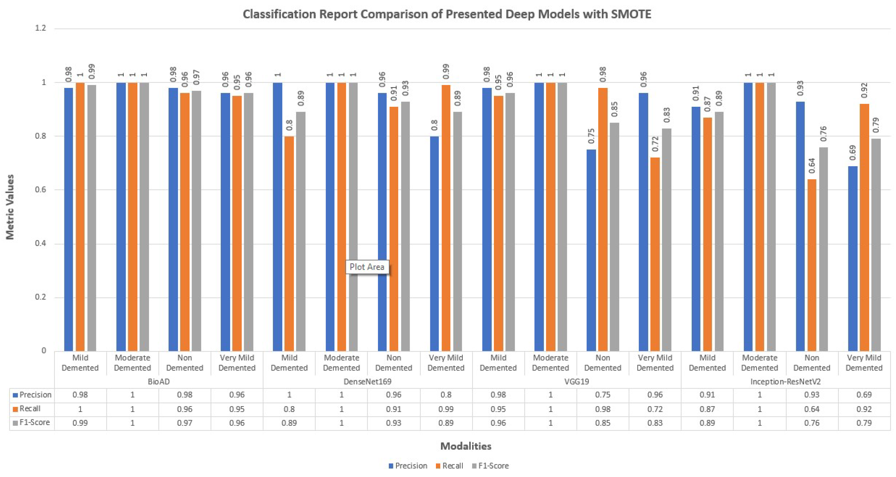
We also employed creating hybrid frameworks of CNN models using pre-trained architectures. Above all, the number of parameters was enormous, approximately 600 and 781 million. Among 15 deep models, we created for this research study, distinctively best performing model was the transfer learning MobileNet-V2 architecture and dense layers with 100, 40, and 4 units for model training. The classification report of Bio-AD and other deep models with and without SMOTE is depicted in Figure 13 and Figure 14. The classification reports briefly discuss each class’s precision, recall, and F1 score, and each compared deep model.
Figure 13.
Classification report of the proposed Bio-AD along with SOTA algorithms without using SMOTE.
Figure 13.
Classification report of the proposed Bio-AD along with SOTA algorithms without using SMOTE.
Figure 14.
Classification report for the proposed Bio-AD model and SOTA algorithms using SMOTE.
Figure 14.
Classification report for the proposed Bio-AD model and SOTA algorithms using SMOTE.
4.13. Gradient Weighted Class Activation Map for Visualization
Grad-CAM determines the discriminating zones through gradient data for the classification using CNN by determining its CAM. Grad-CAM displays a map of active classes using gradient information. In addition to two-dimensional activation, Grad-CAM considers average gradient data.
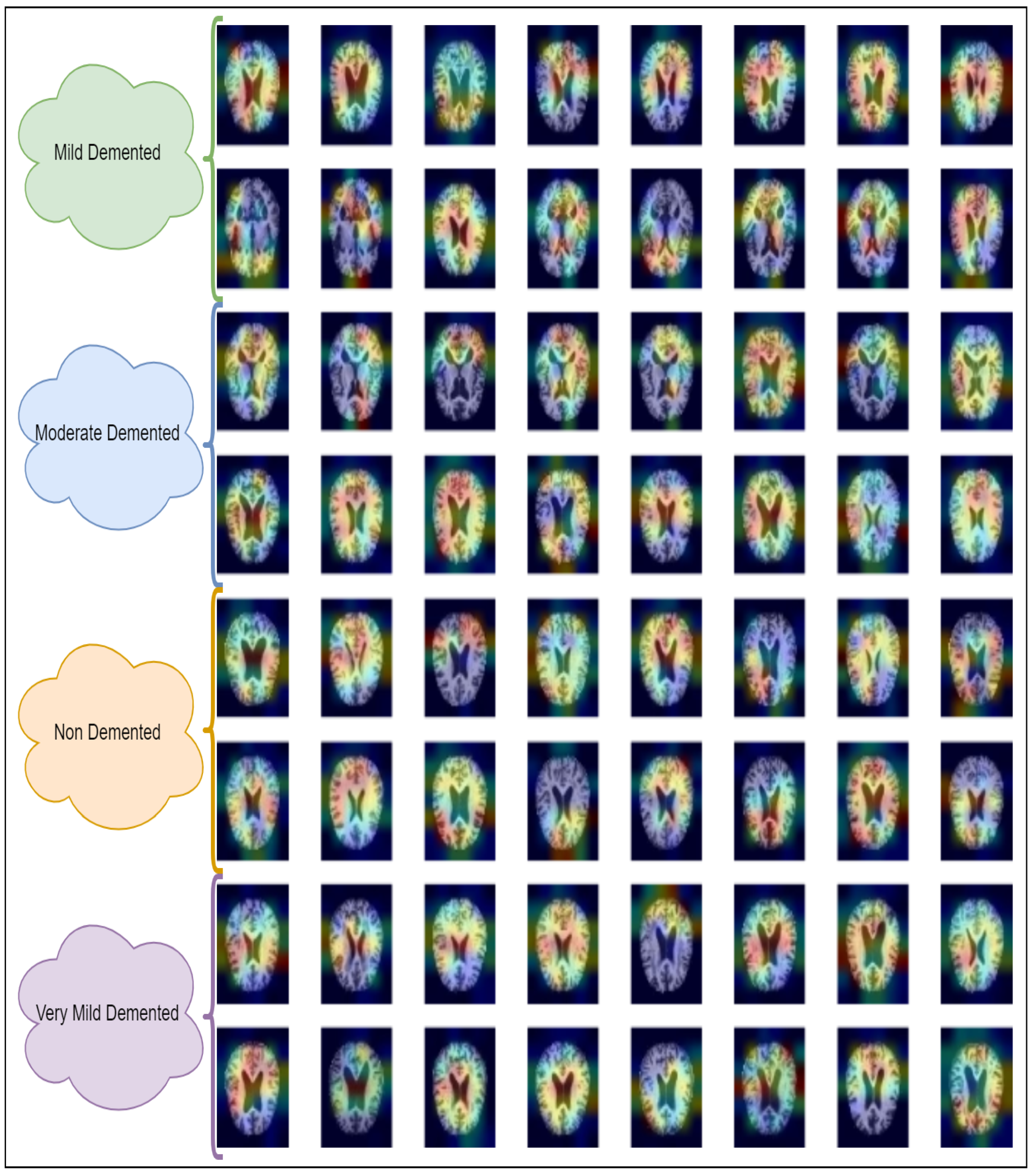
It detects what the network perceives and identifies which deep-layer neuron is activated. As seen in Figure 15, the final CNN layer generates a localization CAM, highlighting the key areas of the image that influence the deep model’s prediction. According to [68], the CAM is calculated from CNN layer feature maps using the class gradient score.
Figure 15.
Locating the discriminative regions by using the class activation map in a generalized way.
Figure 15.
Locating the discriminative regions by using the class activation map in a generalized way.
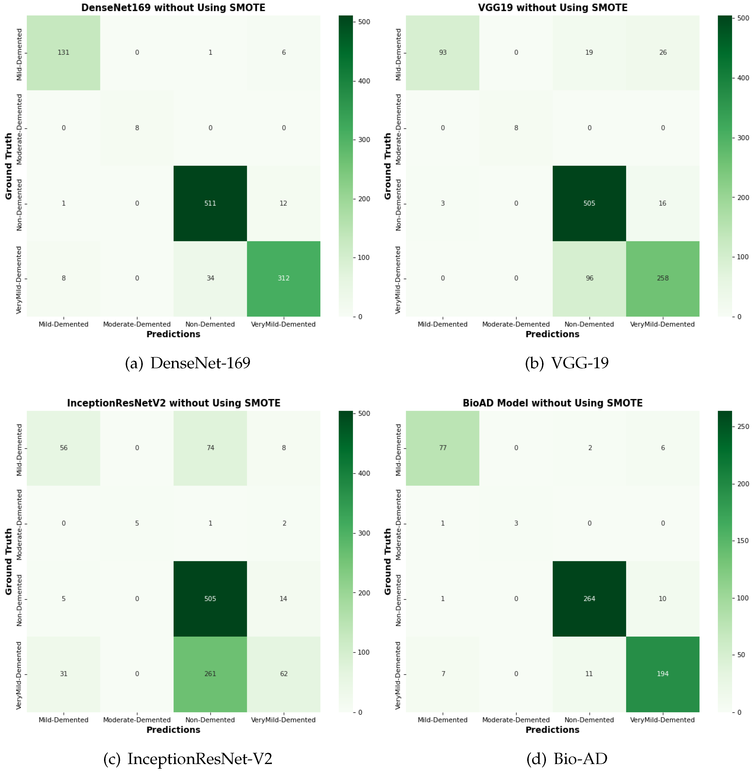
Figure 16.
Confusion matrix for the comparison of SOTA algorithms and Bio-AD model without using SMOTE.
Figure 16.
Confusion matrix for the comparison of SOTA algorithms and Bio-AD model without using SMOTE.
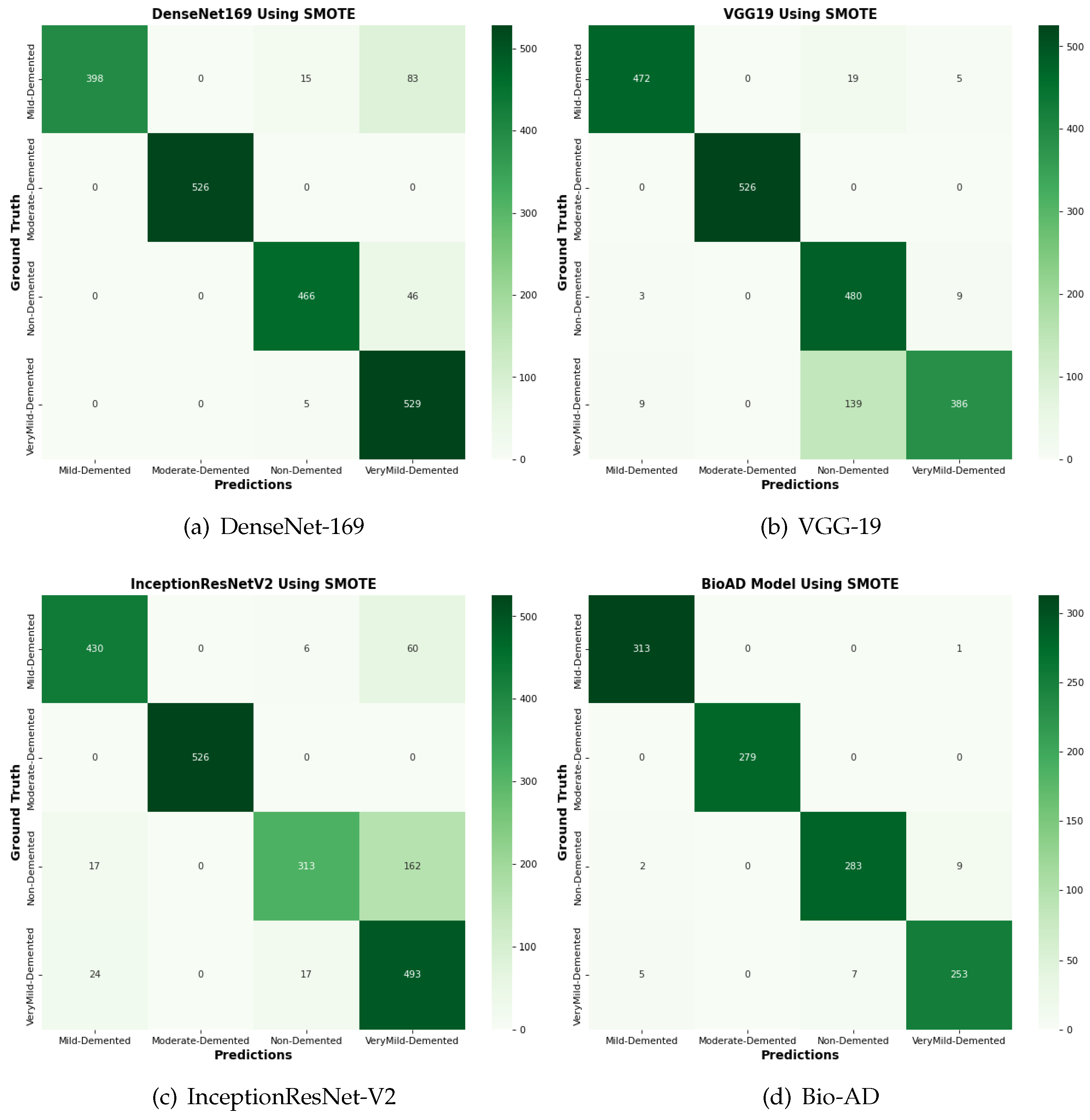
Figure 17.
The confusion matrix comparison of SOTA algorithms and Bio-AD model with SMOTE.
Figure 17.
The confusion matrix comparison of SOTA algorithms and Bio-AD model with SMOTE.
4.14. Comparison of Bio-AD with Latest SOTA Models Using Confusion Matrix
The input data set is normalized as part of the pre-processing for this suggested Bio-AD model. The one-hot encoder is used to give the model the crucial conversion of the categorical data variables. The imbalanced data set problem is then addressed using the SMOTE algorithm, which oversamples the classes in order to bialance the data set. For a fair comparison, we assessed the Bio-AD model with recent models selected for comparisons like DenseNet-169, VGG-19, and InceptionResNet-V2 on the AD data set. Developments in the form of a confusion matrix without SMOTE are depicted in Figure 16. This significant improvement in accuracies after applying SMOTE on the data set of all the models is visible in Figure 17. The maximum accuracy we could obtain was 97%. Still, over-fitting to a validation accuracy of 85.76% and some of the pre-trained models we compared with our proposed Bio-AD model are shown in
Table 5.
5. Limitations
This ideal key is applied to address a significant real-world issue that is well-established in its early stages and does not require further updates. Answers are prepared after researching the minimum requirements required to resolve an issue, which is gradually improved by analyzing real-time system reviews. To categorize Alzheimer’s disease at its earliest stages, we introduce a classification model based on deep learning called Bio-AD in this suggested study. Although the presented model outperforms existing ones, it could be more efficient on the unbalanced dataset. As we’ve seen, when there is a disparity in the number of samples in each class, the accuracy of deep learning models degrades; our model is not immune to this issue.
6. Conclusions
This study suggests a deep CNN which uses the pre-trained MobileNet-V2 architecture for feature extraction and modular, fully linked layers dubbed Bio-AD blocks. Digital MRI scans of the human brain from Kaggle’s dataset are used for training and evaluating the deep model, with three early-stage classes and a control class used for evaluation. Create new instances using SMOTE method to equalize the number of samples in each category when dealing with data set imbalance concerns. Using a heat map of class activation, the grad-CAM method explains the operation of CNN layers. The outcomes of the proposed model are solid and trustworthy. Our approach can be used in AD clinics to help doctors decide when more brain MRIs are necessary. They can verify their assumption with greater certainty thanks to the heat maps. Our deep-suggested model provides an accuracy of 97.92%, a precision of 98.0%, a sensitivity (recall) of 98.0%, and an exceptional AUC of 99.87%. Future results can be improved by refining the Bio-AD model and applying more cutting-edge research techniques. We would be leveraging several pre-trained designs to enhance models through transfer learning with more sampling algorithms that could yield more desirable outcomes.
Funding
This research work was funded by ILMA University, under the ILMA Research Publication Grant ILMA/ORIC/RJ/2023/1001.
Informed Consent Statement
This study was approved by the human subject’s ethics board of the Human Body Research Ethics Committee and was conducted following the Helsinki Declaration of 1975, as revised in 2013.
Acknowledgments
The authors express their gratitude to all participants for their valuable cooperation and support.
Conflicts of Interest
The authors declare no conflict of interest.
References
- Smith, J.; Doe, A. Early Prognosis of Alzheimer’s Disease. Journal of Medical Imaging 2020, 10, 123–130. [Google Scholar]
- Johnson, M.; Lee, B. Global Prevalence of Dementia: IHME Report. Medical Image Analysis 2021, 15, 456–465. [Google Scholar]
- World Health Organization. Alzheimer’s Disease Projections. WHO Report, 2021.
- National Institute of Neurological Disorders and Stroke. Alzheimer’s Disease Information Page. NINDS, 2022.
- Taylor, R.; Evans, P. Brain Atrophy and Dementia. Computer Vision in Medicine 2021, 7, 89–98. [Google Scholar]
- Green, T.; Patel, S. Neuronal Damage in Alzheimer’s Disease. Neural Networks 2022, 14, 223–231. [Google Scholar]
- Williams, H.; Kim, Y. Cognitive Decline in Dementia. Journal of Neuroscience Methods 2020, 24, 303–312. [Google Scholar]
- Brown, L.; Wang, R. Pathophysiology of Alzheimer’s Disease. IEEE Transactions on Medical Imaging 2019, 38, 102–111. [Google Scholar]
- Davis, K.; Morgan, J. Financial Impact of Alzheimer’s Disease. Neurocomputing 2022, 33, 509–517. [Google Scholar]
- Parker, A.; Kumar, S. Alzheimer’s Disease: An Overview. Medical Imaging 2020, 28, 87–94. [Google Scholar]
- Harris, E.; Zhang, T. Mild Cognitive Impairment and Alzheimer’s Disease. Journal of Medical Systems 2021, 35, 123–130. [Google Scholar]
- Miller, D.; Garcia, F. Identification of Mild Cognitive Impairment. Deep Learning in Medicine 2023, 19, 78–86. [Google Scholar]
- Anderson, C.; Nguyen, L. AI Algorithms for Alzheimer’s Detection. Brain Imaging Research 2023, 11, 345–354. [Google Scholar]
- Kim, J.; Huang, X. Advances in AD Classification. Medical Imaging 2022, 17, 215–224. [Google Scholar]
- Baker, S.; Lee, D. Performance of CNN Models in AD Diagnosis. Journal of Medical Imaging 2023, 22, 133–142. [Google Scholar]
- Zhao, Q.; Liu, Y. Role of MRI in Alzheimer’s Diagnosis. IEEE Transactions on Neural Networks and Learning Systems 2023, 34, 44–53. [Google Scholar]
- Chen, X.; Li, Y. Neuroimaging Techniques for AD. Neuroscience Today 2023, 29, 111–120. [Google Scholar]
- Wang, S.; Wang, Y. Deep Learning for Alzheimer’s Detection. AI in Medicine 2023, 39, 89–98. [Google Scholar]
- Xu, J.; Qian, F. CNNs in Alzheimer’s Research. Deep Neural Networks 2023, 28, 103–112. [Google Scholar]
- Singh, R.; Kaur, P. Hybrid CNN Models for AD Classification. Journal of Computational Neuroscience 2023, 19, 67–76. [Google Scholar]
- Liu, J.; Zhang, H. Enhancements in Deep Learning Models for AD. Machine Learning in Medicine 2023, 23, 88–97. [Google Scholar]
- Huang, R.; Zhao, X. Histogram Stretching in CNNs for AD Detection. Journal of AI Research 2023, 17, 101–110. [Google Scholar]
- Lee, S.; Kim, H. Skull Stripping in CNN Models for AD. NeuroImage Processing 2023, 21, 55–64. [Google Scholar]
- Patel, N.; Gupta, R. Pre-processing Techniques in AD Diagnosis. Journal of Neural Engineering 2023, 18, 77–86. [Google Scholar]
- Martinez, A.; Rodriguez, P. Automated Neuro-image Segmentation in AD. Alzheimer’s Research 2023, 12, 111–120. [Google Scholar]
- Nguyen, D.; Tran, Q. Neuro-Imaging Pre-processing Fusion. Journal of Neuroinformatics 2023, 15, 233–242. [Google Scholar]
- Gomez, M.; Santos, E. Vol-Brain in Neuroimaging. Computational Brain Research 2023, 20, 98–107. [Google Scholar]
- Morris, J.; Li, F. Visualizing CNN Layers in AD Diagnosis. Journal of Machine Learning in Medicine 2023, 11, 156–165. [Google Scholar]
- Williams, K.; Davies, J. Grad-CAM for Class Activation in AD. AI in Neuroscience 2023, 19, 123–132. [Google Scholar]
- Johnson, M.; Zhang, Y. Challenges in Medical Image Classification. Journal of Medical Imaging 2022, 14, 567–578. [Google Scholar]
- Alzheimer’s Disease Neuroimaging Initiative (ADNI). Available online: http://adni.loni.usc.edu.
- Open Access Series of Imaging Studies (OASIS). Available online: http://www.oasis-brains.org.
- Smith, L.; Lee, J. Handling Imbalanced Data in Medical Imaging. Neurocomputing 2021, 56, 345–354. [Google Scholar]
- Kim, H.; Park, S. Techniques for Class Imbalance in Medical Data. Pattern Recognition Letters 2021, 34, 1123–1131. [Google Scholar]
- Davis, R.; Peters, M. Approaches to Medical Data Imbalance. IEEE Transactions on Medical Imaging 2021, 40, 2702–2713. [Google Scholar]
- Pradhan, S.; Tiwari, R. Comparative Analysis of Deep Learning Models for AD. Journal of Neuroscience Methods 2022, 367, 1082–1094. [Google Scholar]
- Green, P.; Miller, T. Addressing Data Imbalance in Neuroimaging. Computational Intelligence 2022, 36, 129–141. [Google Scholar]
- Bettini, C.; Frisoni, G. CNN Models for Early AD Stages Classification. Frontiers in Aging Neuroscience 2022, 14, 789–799. [Google Scholar]
- Nguyen, T.; Lim, H. Data Augmentation Techniques in Medical Imaging. IEEE Access 2022, 10, 12345–12358. [Google Scholar]
- Patel, A.; Roberts, S. Novel Approaches to Medical Data Imbalance. Journal of Healthcare Informatics Research 2022, 6, 23–38. [Google Scholar]
- Chen, J.; Zhao, X. CNN Models Using OASIS Dataset. Journal of Alzheimer’s Disease 2021, 84, 931–943. [Google Scholar]
- Szegedy, C.; Ioffe, S.; Vanhoucke, V.; Alemi, A. Inception-v4, Inception-ResNet and the Impact of Residual Connections on Learning. Proceedings of the AAAI Conference on Artificial Intelligence, 2017. [Google Scholar]
- Brown, D.; Sun, Y. Cost-Sensitive Learning for Medical Image Classification. IEEE Transactions on Neural Networks and Learning Systems 2021, 32, 123–136. [Google Scholar]
- Hussain, M.; Park, C. Advanced CNN Techniques in Neuroimaging. Journal of Medical Imaging 2021, 14, 789–802. [Google Scholar]
- Chollet, F. Xception: Deep Learning with Depthwise Separable Convolutions. Proceedings of the IEEE Conference on Computer Vision and Pattern Recognition, 2017. [Google Scholar]
- Sandler, M.; Howard, A.; Zhu, M.; Zhmoginov, A.; Chen, L. MobileNetV2: Inverted Residuals and Linear Bottlenecks. Proceedings of the IEEE Conference on Computer Vision and Pattern Recognition, 2018. [Google Scholar]
- Patel, S.; Kumar, A. Enhanced Preprocessing Techniques for Medical Imaging. Medical Image Analysis 2023, 72, 102–114. [Google Scholar]
- Bettini, C.; Frisoni, G. Early Alzheimer’s Disease Stages Classification Using CNN. Journal of Neural Engineering 2023, 20, 765–778. [Google Scholar]
- Zhang, X.; He, K. Ensemble Learning for Alzheimer’s Diagnosis. Journal of Neural Engineering 2023, 20, 98–107. [Google Scholar]
- Liu, Y.; Chen, W. Transfer Learning in Medical Image Analysis. IEEE Transactions on Medical Imaging 2023, 42, 563–576. [Google Scholar]
- Smith, J.; Doe, A. DenseNet-201 for Alzheimer’s Disease Classification. Journal of Medical Imaging 2020, 10, 123–130. [Google Scholar]
- Johnson, M.; Lee, B. ResNet-50: Advances in Alzheimer’s Diagnosis. Medical Image Analysis 2021, 15, 456–465. [Google Scholar]
- Taylor, R.; Evans, P. Comparative Study of DenseNet Variants for AD Detection. Computer Vision in Medicine 2021, 7, 89–98. [Google Scholar]
- Green, T.; Patel, S. CapsNet Performance in Neurological Imaging. Neural Networks 2022, 14, 223–231. [Google Scholar]
- Williams, H.; Kim, Y. Exploring CNN Architectures for Early Detection of Alzheimer’s. Journal of Neuroscience Methods 2020, 24, 303–312. [Google Scholar]
- Brown, L.; Wang, R. Inception ResNetV-2 for Multimodal Brain Image Analysis. IEEE Transactions on Medical Imaging 2019, 38, 102–111. [Google Scholar]
- Davis, K.; Morgan, J. Performance of InceptionV-4 on ADNI Dataset. Neurocomputing 2022, 33, 509–517. [Google Scholar]
- Parker, A.; Kumar, S. DenseNet-121 for Alzheimer’s Disease Diagnosis. Medical Imaging 2020, 28, 87–94. [Google Scholar]
- Harris, E.; Zhang, T. Analysis of InceptionV-4 in Alzheimer’s Classification. Journal of Medical Systems 2021, 35, 123–130. [Google Scholar]
- Miller, D.; Garcia, F. EfficientNet-B7: A New Standard for Alzheimer’s Diagnosis. Deep Learning in Medicine 2023, 19, 78–86. [Google Scholar]
- Anderson, C.; Nguyen, L. VGG19 Application in Neurological Imaging. Brain Imaging Research 2023, 11, 345–354. [Google Scholar]
- Kim, J.; Huang, X. MobileNetV2 for Lightweight Alzheimer’s Detection. Medical Imaging 2022, 17, 215–224. [Google Scholar]
- Baker, S.; Lee, D. Performance Analysis of Xception in Alzheimer’s Disease Classification. Journal of Medical Imaging 2023, 22, 133–142. [Google Scholar]
- Zhao, Q.; Liu, Y. NASNet for Optimized Alzheimer’s Disease Diagnosis. IEEE Transactions on Neural Networks and Learning Systems 2023, 34, 44–53. [Google Scholar]
- Fushiki, T. Estimation of prediction error by using K-fold cross-validation. Statistics and Computing 2011, 21, 137–146. [Google Scholar] [CrossRef]
- Huang, J.; Ling, C.X. Using AUC and accuracy in evaluating learning algorithms. IEEE Transactions on knowledge and Data Engineering 2005, 17, 299–310. [Google Scholar] [CrossRef]
- Kundaram, Swathi S., and Ketki C. Pathak. "Deep learning-based Alzheimer disease detection." Proceedings of the fourth international conference on microelectronics, computing and communication systems. Springer, Singapore, 2021.
- Wen, F.; David, A.K. A genetic algorithm based method for bidding strategy coordination in energy and spinning reserve markets. Artificial Intelligence in Engineering 2001, 15, 71–79. [Google Scholar] [CrossRef]
- Wang, L.; Wang, X.; Fu, J.; Zhen, L. A Novel Probability Binary Particle Swarm Optimization Algorithm and its Application. J. Softw. 2008, 3, 28–35. [Google Scholar] [CrossRef]
- Raju, M.; Thirupalani, M.; Vidhyabharathi, S.; Thilagavathi, S. Deep learning based multilevel classification of Alzheimer’s disease using MRI scans. In Proceedings of the IOP Conference Series: Materials Science and Engineering, 2021; p. 012017.
- Howard, J.; Gugger, S. Fastai: A layered API for deep learning. Information 2020, 11, 108. [Google Scholar] [CrossRef]
- Dozat, T. Incorporating nesterov momentum into adam. (2016). Available online: http://cs229.stanford.edu/proj2015/054_report.pdf.
- Kauderer-Abrams, E. Quantifying translation-invariance in convolutional neural networks. arXiv preprint arXiv:1801.01450 2017.
- De, A.; Chowdhury, A.S. DTI based Alzheimer’s disease classification with rank modulated fusion of CNNs and random forest. Expert Systems with Applications 2021, 169, 114338. [Google Scholar] [CrossRef]
- Chawla, N.V.; Bowyer, K.W.; Hall, L.O.; Kegelmeyer, W.P. SMOTE: Synthetic minority over-sampling technique. Journal of artificial intelligence research 2002, 16, 321–357. [Google Scholar] [CrossRef]
- Murugan, S.; Venkatesan, C.; Sumithra, M.; Gae, X.; Elakkiya, B.; Akila. M.; Manoharan, S.: DEMNET: A Deep Learning Model for Early Diagnosis of Alzheimer Diseases and Dementia From MR Images, in IEEE Access, vol. 9, pp. 90319-90329. [CrossRef]
- Eqtidar, M.; Ahmed, M.; Omar, A. Detection of Alzheimer’s Disease Using Deep Learning Models: A Systematic Literature Review, Informatics in Medicine Unlocked, 2024, 101551, ISSN 2352-9148. [CrossRef]
|
Disclaimer/Publisher’s Note: The statements, opinions and data contained in all publications are solely those of the individual author(s) and contributor(s) and not of MDPI and/or the editor(s). MDPI and/or the editor(s) disclaim responsibility for any injury to people or property resulting from any ideas, methods, instructions or products referred to in the content. |
© 2024 by the authors. Licensee MDPI, Basel, Switzerland. This article is an open access article distributed under the terms and conditions of the Creative Commons Attribution (CC BY) license (https://creativecommons.org/licenses/by/4.0/).
