Preprint
Article

Epidemic Control: Social Distancing or Antiviral Medications?

Altmetrics

Downloads

77

Views

23

Comments

0

A peer-reviewed article of this preprint also exists.

Submitted:

27 August 2024

Posted:

28 August 2024

You are already at the latest version

Alerts
Abstract
In this study, we investigate different control scenarios through theoretical analysis and numerical simulations. To account for two important types of control for an early ascending stage of an outbreak, social distancing and treatment with antiviral medications, a compartmental model is considered with one control, $u_1(t)$, aimed to lower the disease transmission rate and the other control, $u_2(t)$, aimed to lower the period of infectiousness. In all experiments, the implementation of control strategies reduces the daily cumulative number of cases and successfully "flattens the curve". The reduction in the cumulative cases is achieved by eliminating or delaying new cases. This delay is incredibly valuable as it provides public health organizations with more time to advance antiviral treatments and devise alternative preventive measures. The main theoretical result of the paper, Theorem 3.1, concludes that the optimal control functions, $u_i(t)$, $i=1,2,$ may be increasing until some moment $\tau \in [0, T)$. However, for all $t \in [\tau, T]$, both controls, $u_i(t)$, decline as $t$ approaches $T$ (possibly causing the number of newly infected people to grow). Numerical simulations presented in Section 4 confirm theoretical findings, which indicates that, ideally, around the time $t=\tau$, the control strategy has to be upgraded and a vaccination campaign needs to start to ensure the epidemic wave does not rebound.
Keywords: 
Subject: Computer Science and Mathematics  -   Mathematical and Computational Biology

1. Introduction

Advanced modeling and parameter estimation algorithms form a solid background for the design of optimal strategies to control infectious diseases, which reduces illness and mortality rates. Vaccination, isolation, and public health education are examples of important control techniques that protect people at risk and make effective use of healthcare resources [1,2,3].
Timely control measures can mitigate the impact of outbreaks, prevent widespread transmission, and save lives. For instance, vaccination programs have been instrumental in controlling diseases such as measles, polio, and influenza [4,5]. Quarantine and isolation protocols were key in managing the spread of diseases like Ebola and COVID-19 [6]. Public health campaigns promoting handwashing and sanitation have significantly reduced the transmission of diseases such as cholera and dysentery. The eradication of smallpox is a prime example of how global vaccination campaigns can lead to complete elimination of a disease [7]. Similarly, the rapid response to the H1N1 influenza pandemic in 2009, including the development and distribution of vaccines, helped to control the spread of the virus and reduce its impact [8].
By analyzing data that use different models and algorithms, epidemiologists can forecast future incidence cases and evaluate various control strategies. Systematic preventive measures can help in reducing the spread of diseases. At first glance, choosing healthcare policies seems obvious, but in reality it is a very complicated task. One needs to put forward control strategies that are practical and, at the same time, have manageable consequences. At the onset of COVID-19, lockdowns were helpful, but they were not sustainable long term [9,10,11]. Thus, choosing the best intervention at the right time is critical [12,13].
The study in [14] introduced a two-stage epidemic model for the spread of COVID-19 and proposed optimal control strategies based on actual data and cost considerations. The research underscores the importance of contact tracing and isolation in minimizing the costs and effectively curbing the spread of a disease. Numerical simulations and model analysis provide actionable recommendations for public health authorities, highlighting the critical role of controlling the transmission rate in epidemic management.
The research in [15] modeled the spread of COVID-19 and assessed the impact of social intervention measures during the early outbreak phase, focusing on optimal control strategies and the identifiability of model parameters. It found that optimal control strategies, especially social distancing and self-isolation, significantly reduced transmission rates when implemented early. The study emphasized the importance of structural identifiability for accurate parameter estimation in COVID-19 models. It shows that implementing control measures effectively "flattens the curve" and lowers the burden on healthcare systems.
Another study, [16], focused on an S I R model with saturated incidence and treatment rates, analyzing equilibrium points, bifurcation, and optimal control strategies that utilize vaccination and treatment with antiviral medication in order to contain the outbreak. The authors’ findings, derived from numerical simulations and efficiency analysis, demonstrated that vaccination control stands to reduce the cumulative number of infections more rapidly than control by antiviral treatment. This research underscored the value of mathematical modeling in epidemiology and the strategic implementation of vaccination to prevent disease transmission.

2. Control of an Emerging Disease

In the study of epidemic control, effective management of a disease spread is crucial, particularly at the onset of an outbreak. While the importance of vaccination in fighting infectious diseases is undeniable, it takes time to develop a vaccine for an emerging strain. Various parameters including environmental factors, immunity patterns, and behavioral changes impact the circulation of a virus. Social distancing and personal hygiene measures (non-medical interventions) play an important role in containing the disease at an early ascending stage. By optimizing the implementation of non-medical interventions over time the effectiveness of these interventions can be increased.
Another essential component of control and prevention is treatment with antiviral medications, which allows to reduce the period of infectiousness and/or reduce the disease fatality rate. To account for these two important types of control, we consider the following S I R (Susceptible-Infectious-Removed) model [17] for early disease transmission:
d S d t = β S ( t ) I ( t ) N d I d t = β S ( t ) I ( t ) N γ I ( t ) d R d t = γ I ( t )
In system (1), we assume that individuals who have recovered from the disease gain immunity for the duration of the study and do not return to the susceptible class, S . Additionally, we assume that natural birth and death rates balance one another and the removed class, R , contains individuals who recovered from the disease and those who died. The two disease parameters, β > 0 and γ > 0 are transmission and recovery rates, respectively.
The focus of this research is on introducing optimal controls during initial weeks of a pandemic in order to delay and reduce the daily number of infections. This approach enables health centers and decision-making organizations to implement more effective operations. In what follows, we incorporate two different kinds of control in S I R model [18] resulting in the system d x d t = f ( x , u ) , where
f 1 ( x , u ) : = β ( 1 u 1 ( t ) ) S ( t ) I ( t ) f 2 ( x , u ) : = β ( 1 u 1 ( t ) ) S ( t ) I ( t ) ( γ + ε u 2 ( t ) ) I ( t ) f 3 ( x , u ) : = ( γ + ε u 2 ( t ) ) I ( t ) .
Here S ( t ) : = S ( t ) N , I ( t ) : = I ( t ) N , and R ( t ) : = R ( t ) N are normalized susceptible, infected and removed compartments, respectively, and N is the population of the region at the beginning of the study period. The function u 1 ( t ) represents nonmedical controls (social distancing, remote work, online education, restriction on travel, lockdowns, etc.), while u 2 ( t ) stands for treatment with antiviral medications and other medical interventions. A positive parameter, ε , is the efficacy of antiviral treatments [19]. In the above, x : = [ S , I , R ] , u : = [ u 1 , u 2 ] , and the admissible set for each control function is
U = u i L 1 [ 0 , T ] , 0 u i ( t ) < 1 , i = 1 , 2 .
In (2), the first control, u 1 ( t ) , aims to change the disease transmission rate from β to β ( 1 u 1 ( t ) ) while the second control, u 2 ( t ) , is expected to reduce the period of infectiousness, which is 1 γ in the initial system (1). In combination, the two controls, u 1 ( t ) and u 2 ( t ) , are meant to minimize the force of infection, β ( 1 u 1 ( t ) ) S ( t ) I ( t ) , while keeping the costs at bay. The costs are considered in a general sense, which includes a negative impact on mental health, education, economy and on overall quality of life.
In Lemma 2.1 below we show that following the introduction of a time-dependent transmission rate, β ( t ) : = β ( 1 u 1 ( t ) ) , and a time-dependent recovery rate, γ ( t ) : = γ + ε u 2 ( t ) , the model d x d t = f ( x , u ) in (2) remains well-defined in the sense that the state variables, S ( t ) , I ( t ) , R ( t ) , originating in a positive octant do not leave the octant for all values of t > 0 . The proof of this lemma is similar to the argument in [20], where system (2) was considered with nonmedical controls only (that is, u 2 ( t ) = 0 ).
Lemma 2.1 [20]. Let u i ( t ) , i = 1 , 2 , be admissible control trajectories with x ( t ) satisfying d x d t = f ( x , u ) given by (2) and
( S ( 0 ) , I ( 0 ) , R ( 0 ) ) Δ 2 : = { ( z 1 , z 2 , z 3 ) R 3 : z 1 + z 2 + z 3 = 1 , z 1 , z 2 , z 3 0 } ,
the probability simplex in R 3 . Then ( S ( t ) , I ( t ) , R ( t ) ) Δ 2 for all t 0 .
Note that the argument in [20] implies that the conclusion of Lemma 2.1 is not limited to β ( t ) : = β ( 1 u 1 ( t ) ) and γ ( t ) : = γ + ε u 2 ( t ) . It is valid for any integrable nonnegative functions β ( t ) and γ ( t ) . To optimize the implementation of both controls, u 1 ( t ) and u 2 ( t ) , we consider the following objective functional
J ( x , u ) : = 0 T ( β ( 1 u 1 ( t ) ) S ( t ) I ( t ) + λ C ( u ( t ) ) d t .
According to system (2), one can integrate the first term to obtain
J ( x , u ) = S ( 0 ) S ( T ) + 0 T λ C ( u ( t ) ) d t : = h ( x ( T ) ) + 0 T L ( x ( t ) , u ( t ) ) d t ,
where C ( u ) : = [ C 1 ( u 1 ) , C 2 ( u 2 ) ] is the assumed cost of control and λ : = [ λ 1 , λ 2 ] , λ 1 , λ 2 > 0 , is the regularization parameter (weight). As our numerical experiments show, the choice of the cost function, C ( u ) , significantly influences the resulting control strategy. From practical standpoint, neither u 1 ( t ) nor u 2 ( t ) should take negative values. At the same time, the cost, C i ( u i ) , must increase dramatically as u i ( t ) approaches 1, the upper bound of the feasible set (3), since it is impossible to entirely eliminate the disease transmission ( u 1 ( t ) = 1 ) . It is equally impossible to reach full capacity of antiviral treatment ( u 2 ( t ) = 1 ) due to limitations of testing and other factors. Therefore, in our approach we impose the following assumptions on the cost functions, C 1 ( u 1 ) and C 2 ( u 2 ) [20]:
C i ( u ) > 0 , C i ( 0 ) = 0 , C i ( u ) > 0 for u > 0 , C i ( u ) < 0 for u < 0 and lim u 1 C i ( u ) = , i = 1 , 2 .
These assumptions on the cost of control were first proposed in [20] for a special case when u 2 ( t ) = 0 . The authors of [20] employed the techniques of machine learning to show that under assumptions (5), the global minimum of the Hamiltonian gives rise to the optimal control strategy, u 1 ( t ) , which stays within the feasible set (3) for all values of t [ 0 , T ] . Assumptions (5) are the alternative to a more traditional cost function, C ( u ) = u 2 , that is often used in control literature. However, C ( u ) = u 2 does not, generally, prevent the global minimum from becoming greater than 1 for some values of t, even for large weights, λ .

3. Theoretical Study and Discussion

In this section we state and prove our main theoretical result.
Theorem 3.1. Let u U be an optimal control strategy with respect to the objective functional J ( x , u ) defined in (4) and biological model x ˙ = f ( x , u ) , x ( 0 ) = x 0 , introduced in (2), with C ( u ) : = [ C 1 ( u 1 ) , C 2 ( u 2 ) ] satisfying (5) and λ : = [ λ 1 , λ 2 ] , λ 1 , λ 2 > 0 . Then there is τ [ 0 , T ) such that for any t ( τ , T ) , the derivative, d u i d t , i = 1 , 2 , exists and d u i d t < 0 . In other words, there is τ [ 0 , T ) such that for any t ( τ , T ) , both optimal controls, u 1 ( t ) and u 2 ( t ) , are decreasing.
Proof. According to the Pontryagin’s Minimum Principle [21,22], if u U is an optimal control with respect to the objective functional J ( x , u ) = h ( x ( T ) ) + 0 T L ( x ( t ) , u ( t ) ) d t and the system x ˙ = f ( x , u ) , x ( 0 ) = x 0 , then there is a trajectory p ( t ) such that
p ˙ ( t ) = x H ( x , u , p ) x ( t ) , u ( t ) , p ( t ) , p ( T ) = x h ( x ) x ( T ) ,
u ( t ) = arg min v U H ( x ( t ) , v ( t ) , p ( t ) ) , H ( x , v , p ) : = L ( x , v ) + p f ( x , v ) .
By the properties (5) of the cost, C ( u ) , one has C i ( u ) > 0 for u > 0 and lim u 1 C i ( u ) = , which prevents any u = [ u 1 , u 2 ] , u i 1 , i = 1 , 2 , from being the optimal of H ( x , u , p ) with respect to u at any time t [ 0 , T ] . Therefore, the Karush–Kuhn–Tucker (KKT) conditions for the optimal control problem (2), (3), (4) take the form
( K 1 ) u H ( x , u , p ) q ( t ) = 0 , q ( t ) : = [ q 1 ( t ) , q 2 ( t ) ]
( K 2 ) p ˙ ( t ) = x H ( x , u , p ) x ( t ) , u ( t ) , p ( t ) , p ( T ) = x h ( x ) x ( T )
( K 3 ) x ˙ ( t ) = f ( x , u ) , x ( 0 ) = x 0
( K 4 ) q i ( t ) 0 , u i ( t ) 0 , i = 1 , 2 , q ( t ) u ( t ) = 0 t [ 0 , T ] .
As it follows from (2), (4), and (7),
u H ( x , u , p ) = u L ( x , u ) + p u f ( x , u )
= L u 1 L u 2 + [ p 1 , p 2 , p 3 ] f 1 u 1 f 1 u 2 f 2 u 1 f 2 u 2 f 3 u 1 f 3 u 2
= λ 1 d c 1 d u 1 λ 2 d c 2 d u 2 + [ p 1 , p 2 , p 3 ] β S I 0 β S I ε I 0 ε I ,
which yields
λ 1 d c 1 d u 1 q 1 ( t ) = β ( p 1 p 2 ) S I
λ 2 d c 2 d u 2 q 2 ( t ) = ε ( p 3 p 2 ) I .
To show that on some ( τ , T ) the derivative, d u 1 d t , exists and d u 1 d t < 0 , we follow [20]. Conditions (K2) and (K3) imply that ( p 1 p 2 ) S I is differentiable and therefore continuous for any t [ 0 , T ] . From Lemma 2.1, one concludes that S ( t ) , I ( t ) > 0 as long as S ( 0 ) and I ( 0 ) are positive. On the other hand, since p 1 ( T ) = 1 < 0 = p 2 ( T ) , there is τ 1 [ 0 , T ) such that p 1 ( t ) p 2 ( t ) < 0 for all t [ τ 1 , T ) . Suppose at some point t [ τ 1 , T ] , the Lagrange multiplier, q 1 ( t ) , is greater than zero. Then from (K4) it follows that u 1 ( t ) = 0 . By (5), this implies d c 1 d u 1 ( t ) = 0 , which means that in (14) d c 1 d u 1 ( t ) q 1 ( t ) < 0 , while β ( p 1 p 2 ) S I > 0 . Hence, we arrive at the contradiction. Therefore, for any t [ τ 1 , T ] , one has q 1 ( t ) = 0 and λ 1 d c 1 d u 1 = β ( p 1 p 2 ) S I . By implicit function theorem, for t ( τ 1 , T ) the derivative, d u 1 d t , exists and
d u 1 d t = β [ S ( t ) I ( t ) ( p 1 ( t ) p 2 ( t ) ) ] λ 1 c 1 ( u 1 ) f o r a l l t ( τ 1 , T ) .
Taking into consideration (2), (4), and (7), one obtains
x H ( x , u , p ) = x L ( x , u ) + p x f ( x , u )
= L S L I L R + [ p 1 , p 2 , p 3 ] f 1 S f 1 I f 1 R f 2 S f 2 I f 2 R f 3 S f 3 I f 3 R
= 0 0 0 + [ p 1 , p 2 , p 3 ] β ( 1 u 1 ) I β ( 1 u 1 ) S 0 β ( 1 u 1 ) I β ( 1 u 1 ) S ( γ + ε u 2 ) 0 0 ( γ + ε u 2 ) 0 .
Furthermore, from (4) one gets x h ( x ) = [ 1 , 0 , 0 ] . This together with (16) implies that p 3 ( t ) = 0 and the costate equations for p 1 ( t ) and p 2 ( t ) take the form:
p ˙ 1 = β ( 1 u 1 ( t ) ) ( p 1 ( t ) p 2 ( t ) ) I ( t ) p ˙ 2 = β ( 1 u 1 ( t ) ) ( p 1 ( t ) p 2 ( t ) ) S ( t ) + p 2 ( t ) ( γ + ε u 2 ( t ) ) p 1 ( T ) = 1 , p 2 ( T ) = 0 .
Combining (2) and (17), one can rewrite [ S ( t ) I ( t ) ( p 1 ( t ) p 2 ( t ) ) ] as follows
[ S ( t ) I ( t ) ( p 1 ( t ) p 2 ( t ) ) ] = ( S I + S I ) ( p 1 p 2 ) + ( p 1 p 2 ) S ( t ) I ( t ) = β ( 1 u 1 ) S I 2 + β ( 1 u 1 ) S 2 I ( γ + ε u 2 ) S I ( p 1 p 2 ) + β ( p 1 p 2 ) ( 1 u 1 ) ( I S ) p 2 ( γ + ε u 2 ) S I = p 1 ( γ + ε u 2 ) S I .
From (24) and (15), one concludes
d u 1 d t = β p 1 ( γ + ε u 2 ) S I λ 1 c 1 ( u 1 ) f o r a l l t ( τ 1 , T ) .
Since p 1 ( T ) = 1 < 0 and S ( t ) , I ( t ) > 0 , γ + ε u 2 > 0 , λ 1 c 1 ( u 1 ) > 0 for t [ 0 , T ] , there exists τ 2 [ 0 , T ) such that p 1 ( t ) < 0 and β p 1 ( γ + ε u 2 ) S I λ 1 c 1 ( u 1 ) < 0 for all t [ τ 2 , T ] . Let τ = max ( τ 1 , τ 2 ) , then d u 1 d t is negative in ( τ , T ) . As noted above, p 3 ( t ) = 0 , therefore identity (14) yields
λ 2 d c 2 d u 2 q 2 ( t ) = ε p 2 I .
Taking into account (17), one arrives at
d d t p 2 ( t ) e t T ( γ + ε u 2 ( μ ) ) d μ = β ( 1 u 1 ( t ) ) ( p 1 ( t ) p 2 ( t ) ) S ( t ) e t T ( γ + ε u 2 ( μ ) ) d μ .
Integrating (21) from t to T and substituting p ( T ) = 0 , one gets
p 2 ( t ) = β e t T ( γ + ε u 2 ( μ ) ) d μ t T ( 1 u 1 ( ν ) ) ( p 1 ( ν ) p 2 ( ν ) ) S ( ν ) e ν T ( γ + ε u 2 ( μ ) ) d μ d ν .
As shown above, p 1 ( t ) p 2 ( t ) is negative on [ τ , T ] . Thus (3) and (22) imply that p 2 ( t ) > 0 for all t [ τ , T ) . Using the same argument as in the case of u 1 ( t ) , one can now conclude that q 2 ( t ) in (20) is equal to zero on [ τ , T ] , that is, the constraint u 2 ( t ) 0 is not active for t [ τ , T ) and λ 2 d c 2 d u 2 = ε p 2 I . By implicit function theorem, for t ( τ , T ) the derivative, d u 2 d t , exists and
d u 2 d t = ε [ p 2 I ] λ 2 c 2 ( u 2 ) f o r a l l t ( τ , T ) .
From (2) and (17) one has
[ p 2 I ] = β ( 1 u 1 ) ( p 1 p 2 ) S + p 2 ( γ + ε u 2 ) I + p 2 β ( 1 u 1 ) S I ( γ + ε u 2 ) I .
= β p 1 ( 1 u 1 ) S I < 0 o n [ τ , T ] ,
since p 1 ( t ) < 0 for all t [ τ 2 , T ] and τ τ 2 . This implies d u 2 d t < 0 in ( τ , T ) , which completes the proof. □
Remark 3.2 By (5) and (7), u 2 H ( x , u , p ) = λ 1 c 1 ( u 1 ) 0 0 λ 2 c 2 ( u 2 ) . Therefore, u 2 H ( x , u , p ) is positive definite and H ( x , u , p ) has a unique global minimum with respect to u . From the proof of Theorem 3.1, it follows that both coordinates of the global minimum, u 1 ( t ) and u 2 ( t ) , are guaranteed to be less than 1, pointwisely, but they are not guaranteed to be greater than 0 necessarily, which means the solution to our optimal control problem can be a local minimum rather than global. The reason the coordinates of the global minimum, u i ( t ) , i = 1 , 2 , can potentially be less than zero for some values of t is that, counterintuitively, a smaller effective reproduction number, r ( t ) , in the SIR model does not always imply a smaller cumulative number of infected people, S ( 0 ) S ( t ) . Hence, even though for system (2), the effective reproduction number, r ( t ) = β ( 1 u 1 ( t ) ) / ( γ + ε u 2 ( t ) ) , goes down with more control, it does not guarantee that r ( t ) r ¯ ( t ) yields S ( t ) S ¯ ( t ) for every value of t. One can, however, show that if r ( t ) r ¯ ( t ) and r ( t ) is non-increasing, then S ( t ) S ¯ ( t ) . This result is important in its own right. Its proof is given in Appendix.
Remark 3.3 Despite the fact that, theoretically, the solution to our optimal control problem can be a local minimum rather than global, in all numerical experiments presented in the next section, the optimal strategy is a unique global minimum. In other words, in all our experiments, the optimal control has been computed from the first-order necessary condition for unconstrained minimization, and nonnegativity constraints held without being enforced. For all cost functions, C ( u ( t ) ) , satisfying (5), the global minimum of H ( x , u , p ) with respect to u has nonnegative coordinates, u i ( t ) , i = 1 , 2 . That is, u ( t ) = arg min v U H ( x ( t ) , v ( t ) , p ( t ) ) is equivalent to u ( t ) = arg min v L 1 [ 0 , T ] H ( x ( t ) , v ( t ) , p ( t ) ) for all t [ 0 , T ] . This illustrates that conditions (5) lead to a practically justified mitigation scenario. Numerical simulations have also confirmed, as proven in Theorem 3.1, that both controls, u 1 ( t ) and u 2 ( t ) , are decreasing toward the end of the study period.

4. Numerical Experiments

In our numerical study, we use a second-order trust-region algorithm for nonlinear optimization ’lsqnonlin’ combined with ode15s built-in function to approximate the solution to optimal control problem (4) subject to compartmental model (2) and costate system (17). For every value of u k , we solve system (2) forward in time (starting with x ( 0 ) = x 0 ), to get x k using ode15s. Then system (17) is solved back in time by ode15s to obtain p k . Given ( x k , u k , p k ) , we find u k + 1 by applying a second-order trust-region ’lsqnonlin’ algorithm.
Following [20], we consider three different cost functions, C i , 1 , C i , 2 , and C i , 3 , satisfying conditions (5):
C i , 1 ( u ) = 0.830071 ln ( 1 u 2 ) , C i , 2 ( u ) = 0.672850 u ln ( 1 u ) C i , 3 ( u ) = u ln ( 1 u ) , C i , 4 ( u ) = 1.424546 u 2 i = 1 , 2 .
In (26), the coefficients are chosen to minimize the weighted distance [20]
0 1 w ( z ) | C i , j ( z ) C i , 3 ( z ) | 2 d z , w ( z ) = 1 z 2 , j = 1 , 2 , 4 .
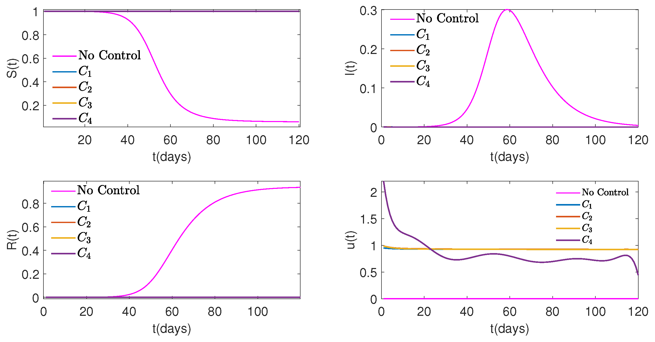
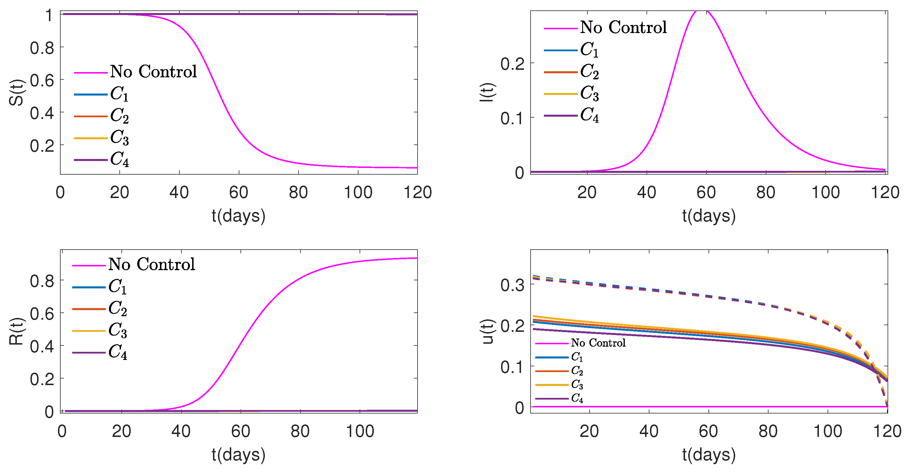
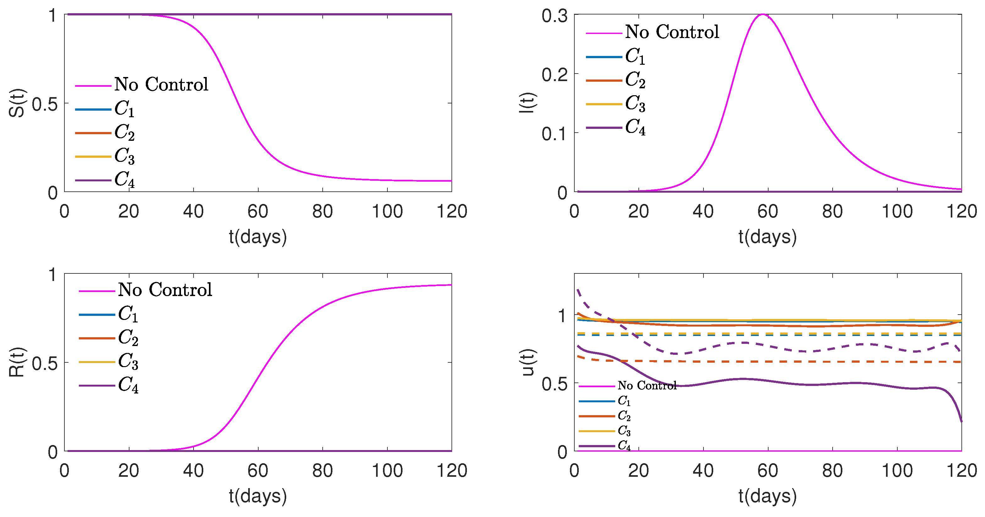
The cost of control, C i , 1 ( u ) , C i , 2 ( u ) , and C i , 3 ( u ) , is infinite as u approaches its ultimate value, 1. For comparison, we also use the cost function C i , 4 ( u ) = u 2 , for which (5) does not hold. The cost function C i , 4 ( u ) = u 2 is popular in applications of control theory in epidemiology and other fields, since for this function the first order optimality condition is linear with respect to u. This is a useful property that simplifies numerical algorithms. However, the cost of control, C i , 4 ( u ) , is finite at u = 1 , which is not realistic in real-world scenarios. Figure 4 and Figure 7 show that the global minimum, u ( t ) , of the Hamiltonian, H ( x ( t ) , u ( t ) , p ( t ) ) , does not stay in the range of [ 0 , 1 ] if the cost is given by C i , 4 ( u ) = u 2 , especially for small values of λ i , i = 1 , 2 . Thus, an explicit constraint u i ( t ) 1 must be imposed in the case of C i , 4 ( u ) . Even with the constraint u i ( t ) 1 , the optimal control function, u ( t ) , often reaches the ultimate level [15], u i ( t ) = 1 , which is not practical.
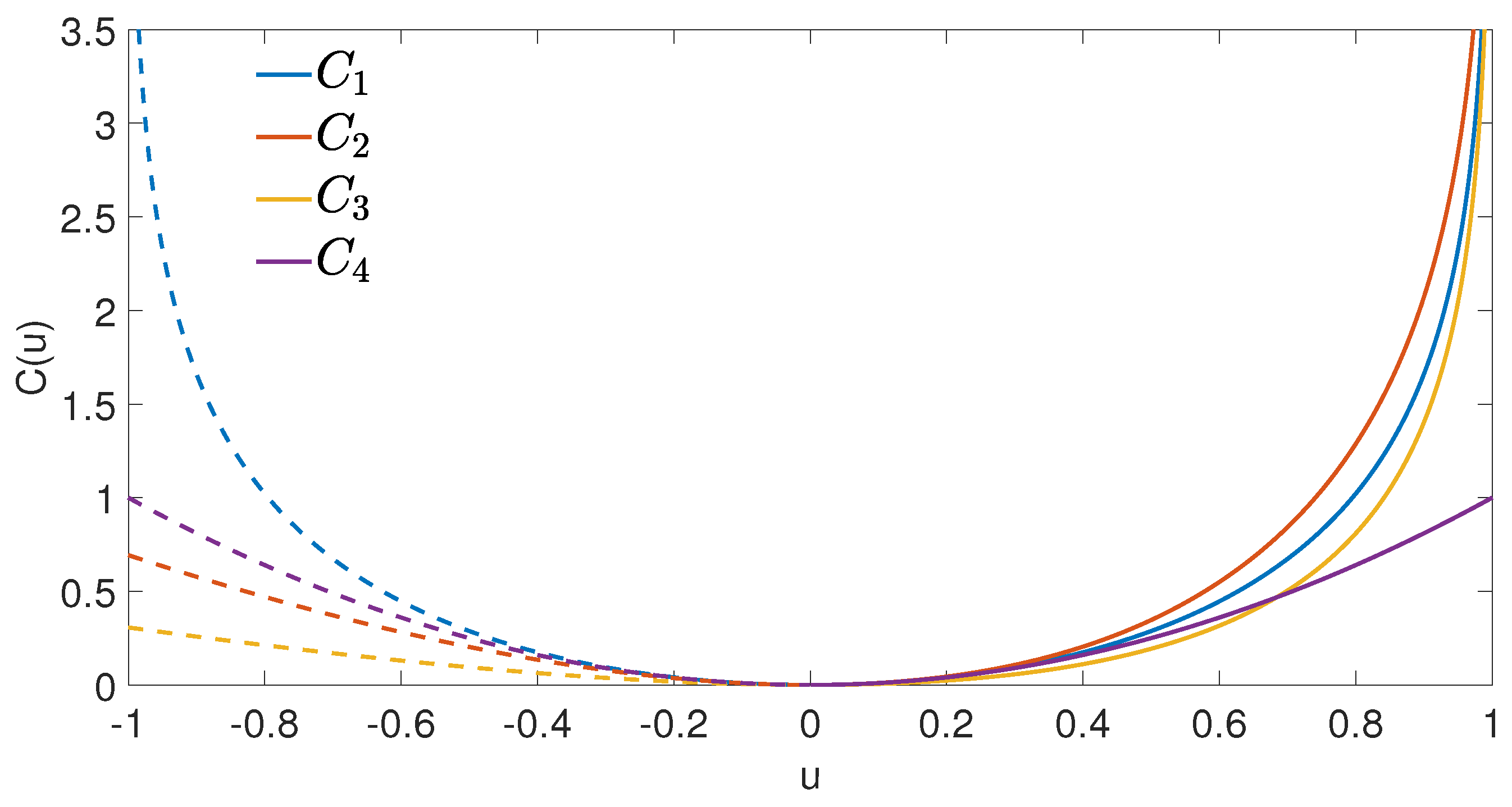
In all numerical experiments presented in this section, C 1 , j ( u ) = C 2 , j ( u ) , j = 1 , 2 , 3 , 4 . Therefore, moving forward, we omit the first index and set C i , j ( u ) : = C j ( u ) . Comparison of the four cost functions in the interval [ 1 , 1 ] is illustrated in Figure 1.
In this study, numerical simulations are conducted for λ 1 and λ 2 equal to 0.1 , 0.05 , 0.01 , 0.001 and 10 7 . Three different scenarios are explored. First, there is only non-medical control, u 1 ( t ) , (social distancing, behavioral changes, hand washing, etc.) in the system and treatment with antiviral medications, u 2 ( t ) , is not available. Second, only control u 2 ( t ) , treatment with antiviral medications, is applied; no social distancing. And third, controls u 1 ( t ) and u 2 ( t ) , medical and non-medical, are used in combination. In our experiments, the population of the region, N, is assumed to be 10 7 . The initial number of infected individuals on day 1 is 200, and the duration of the study period is 120 days. Transmission rate, β , and recovery rate, γ , are assumed to be 0.3 , and 0.1 , respectively, leading to the basic reproduction number r = 3 . The efficacy of antiviral medication, ε , is assumed to be 0.5 when applicable.

4.1. Scenario 1: Social Distancing Control Only

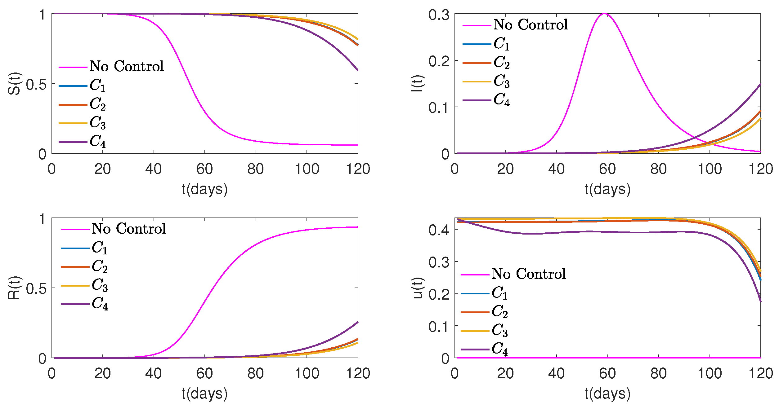
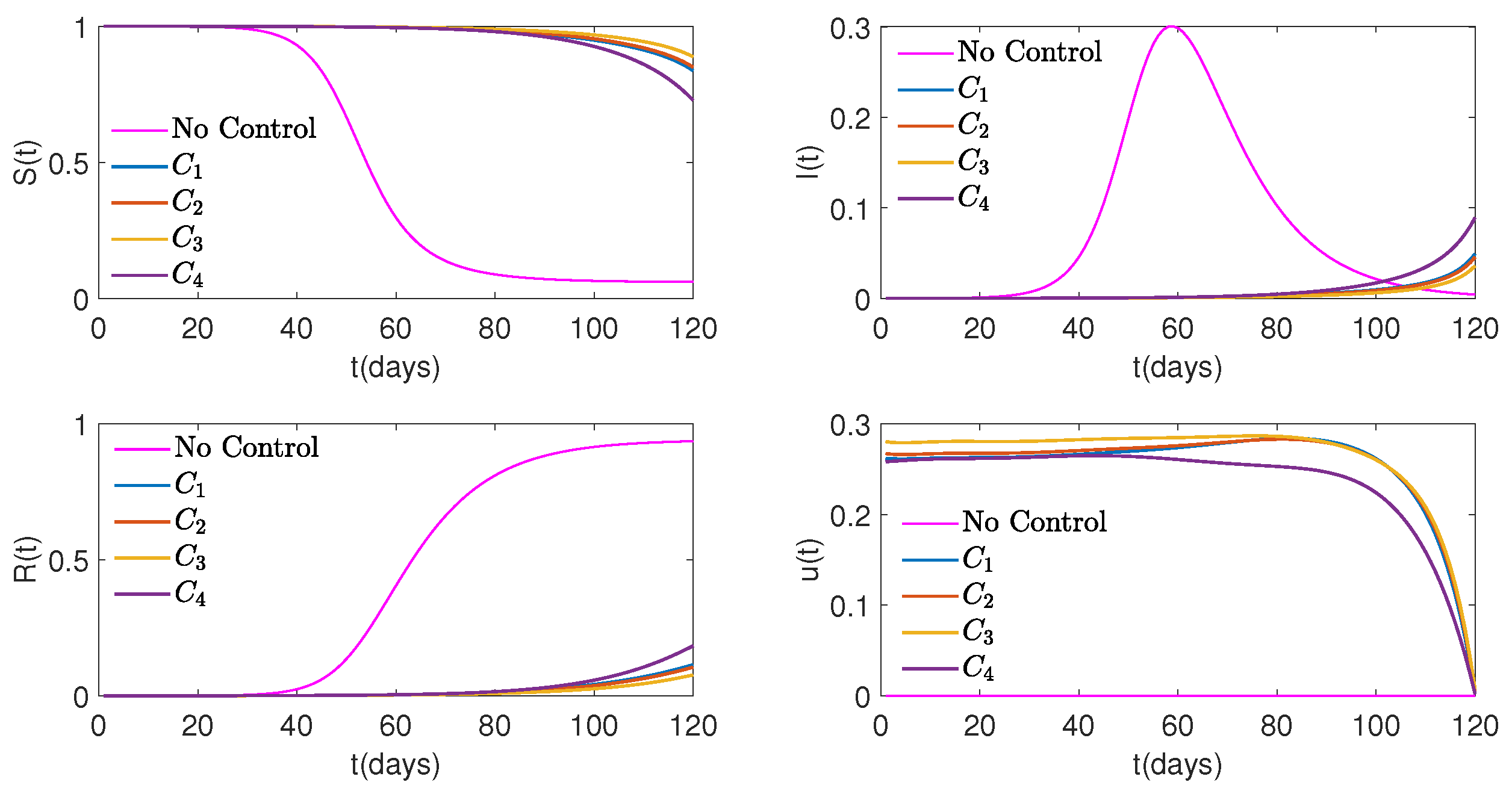
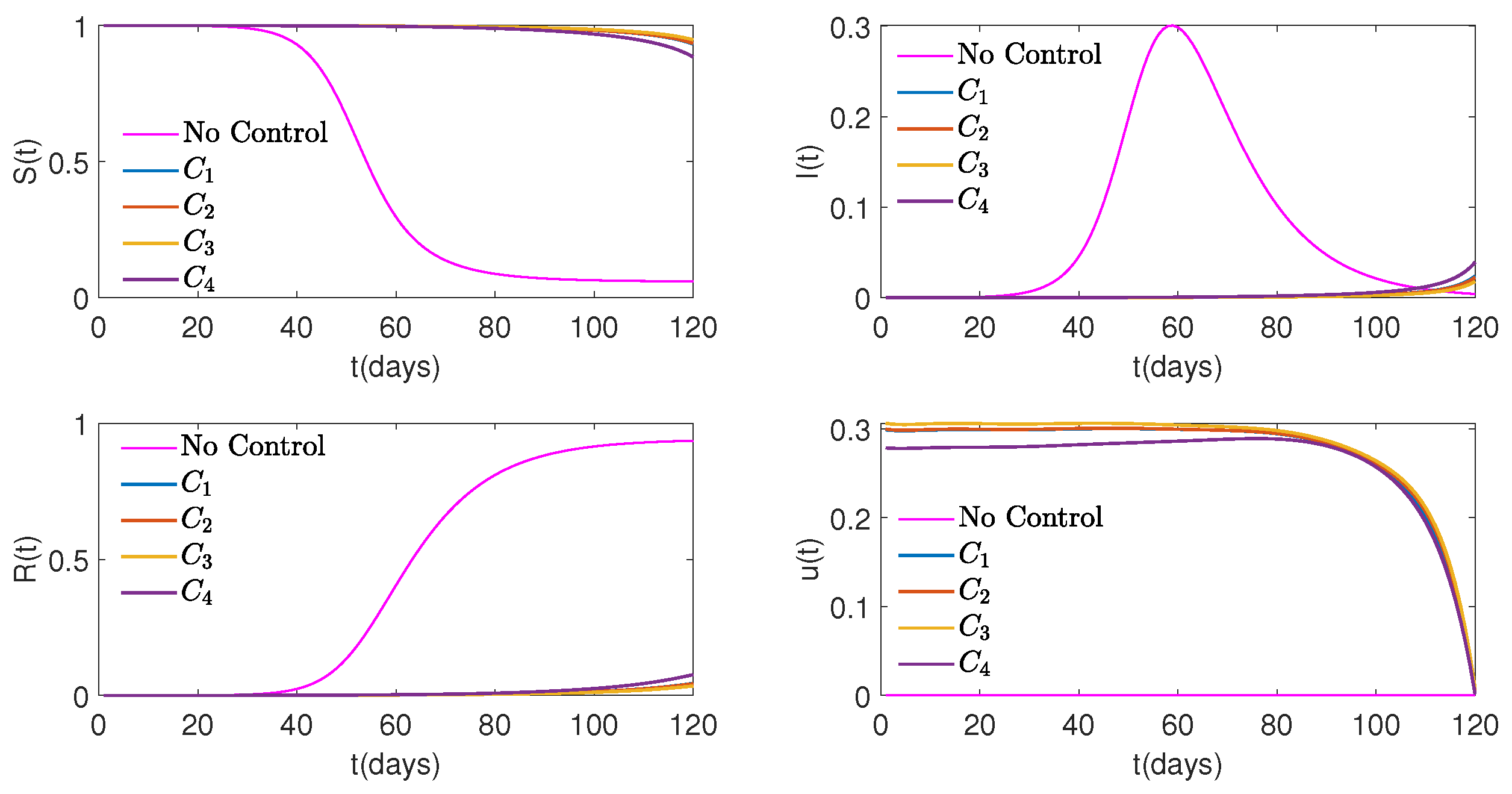
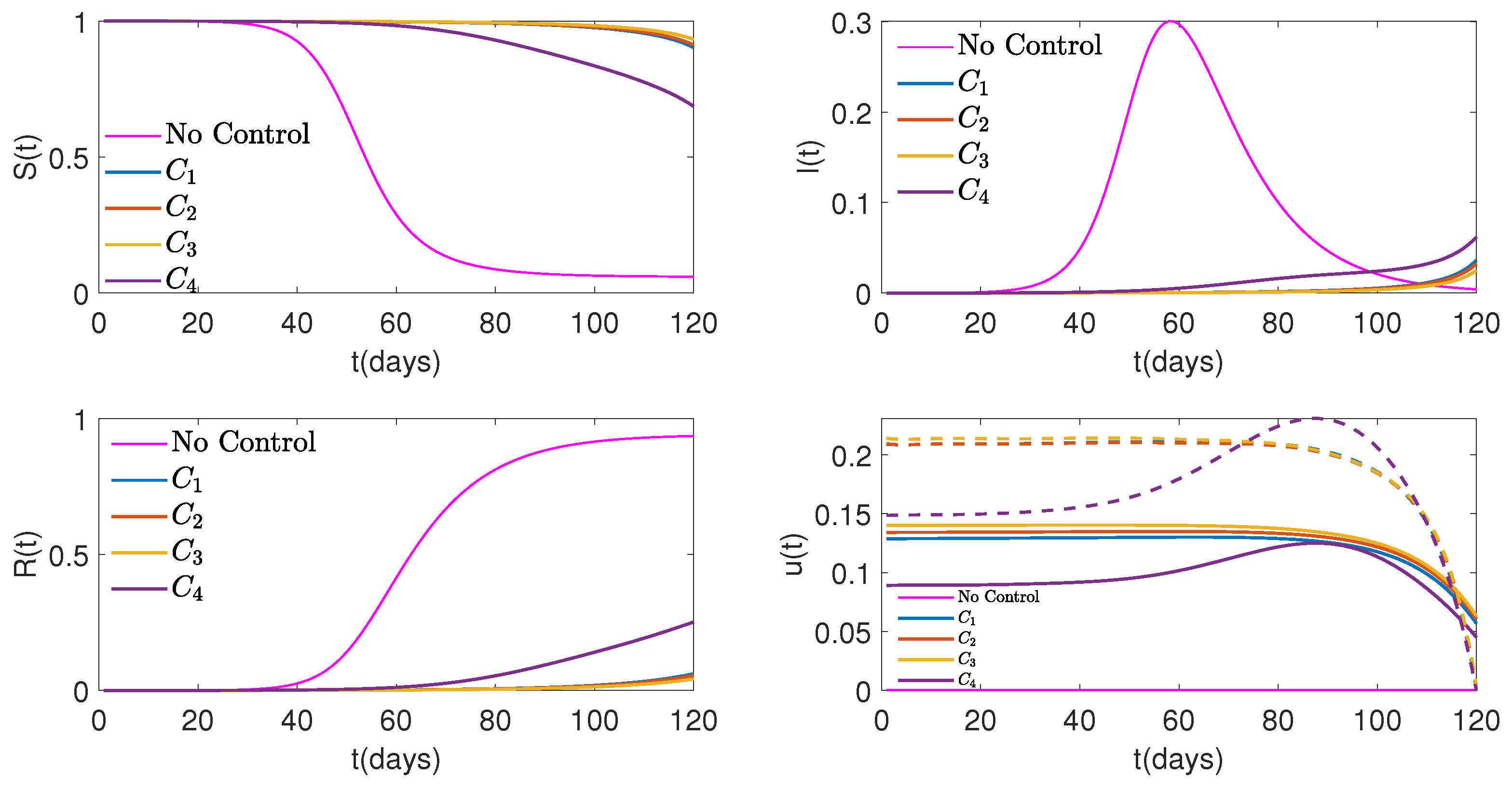
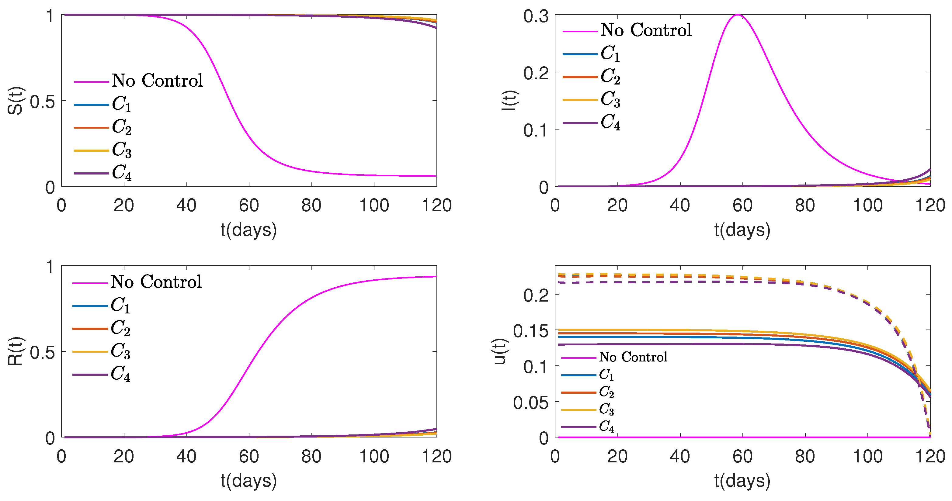
In the first scenario, only one (non-medical) control, u 1 ( t ) , is applied (Figure 2, Figure 3, and Figure 4). As one can see in the figures, when the weight of control, λ 1 , increases, the effectiveness of control goes down; see also Table 1 that illustrates how I ( t ) changes over time for the cost C 1 ( u ) with different values of λ 1 (find similar Tables for C 2 , C 3 , and C 4 in the Appendix). One can conclude from Figure 2 that control u 1 ( t ) works by eliminating some cases but also by delaying some of them. Therefore, even though the cumulative number of infections in the controlled environment is significantly less than in the environment with no control, towards the end of the study period the daily number of infected individuals in the controlled environment may be higher.
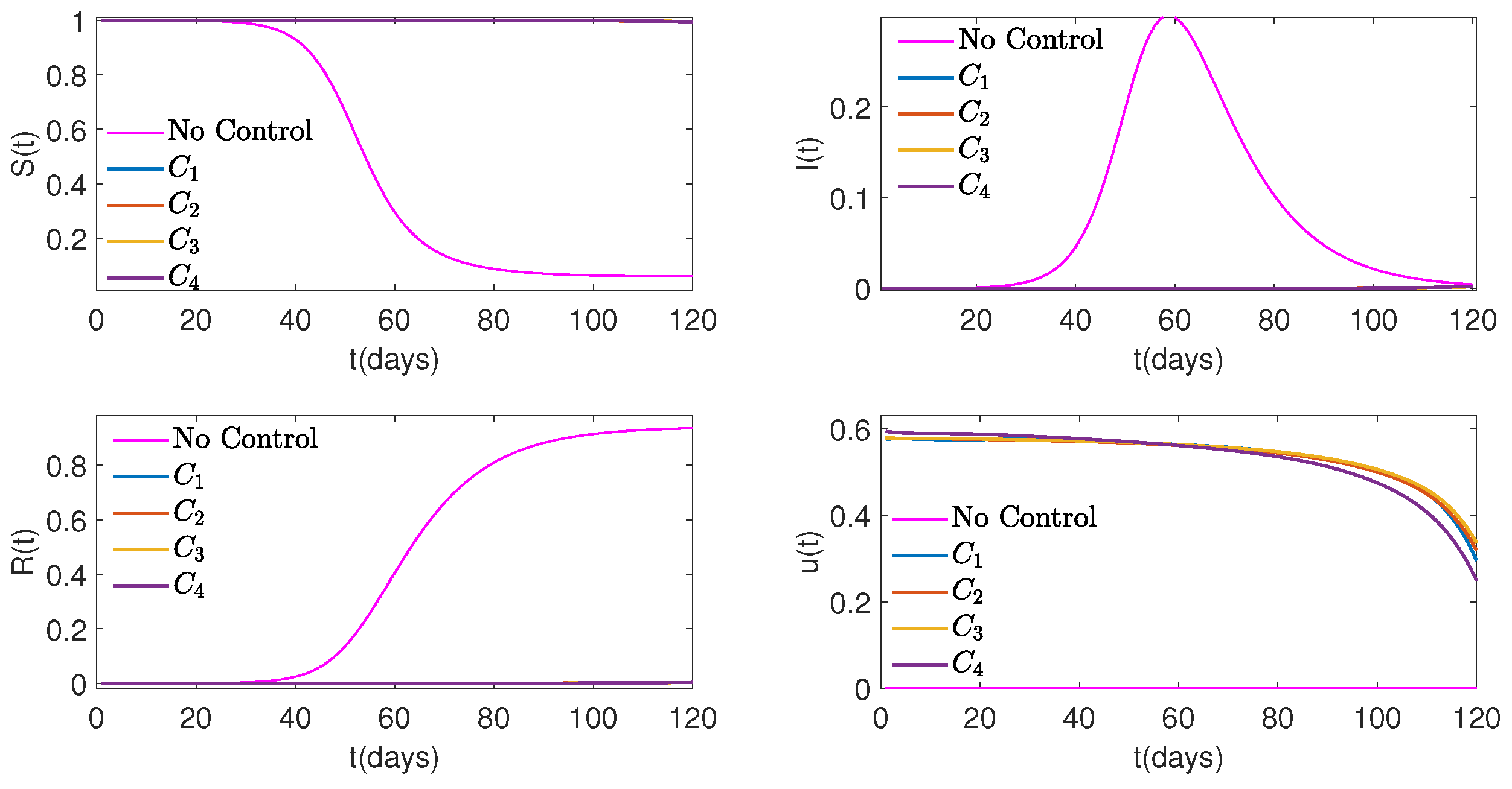
Figure 2, Figure 3, and Figure 4 with λ 1 equal to 0.05 , 0.001 , and 10 7 , respectively, show the pattern of I ( t ) decreasing as the values of λ 1 go down. Based on these figures and Table 1, the "flattening of the curve" is evident.

4.2. Scenario 2: Control with Antiviral Medication Only

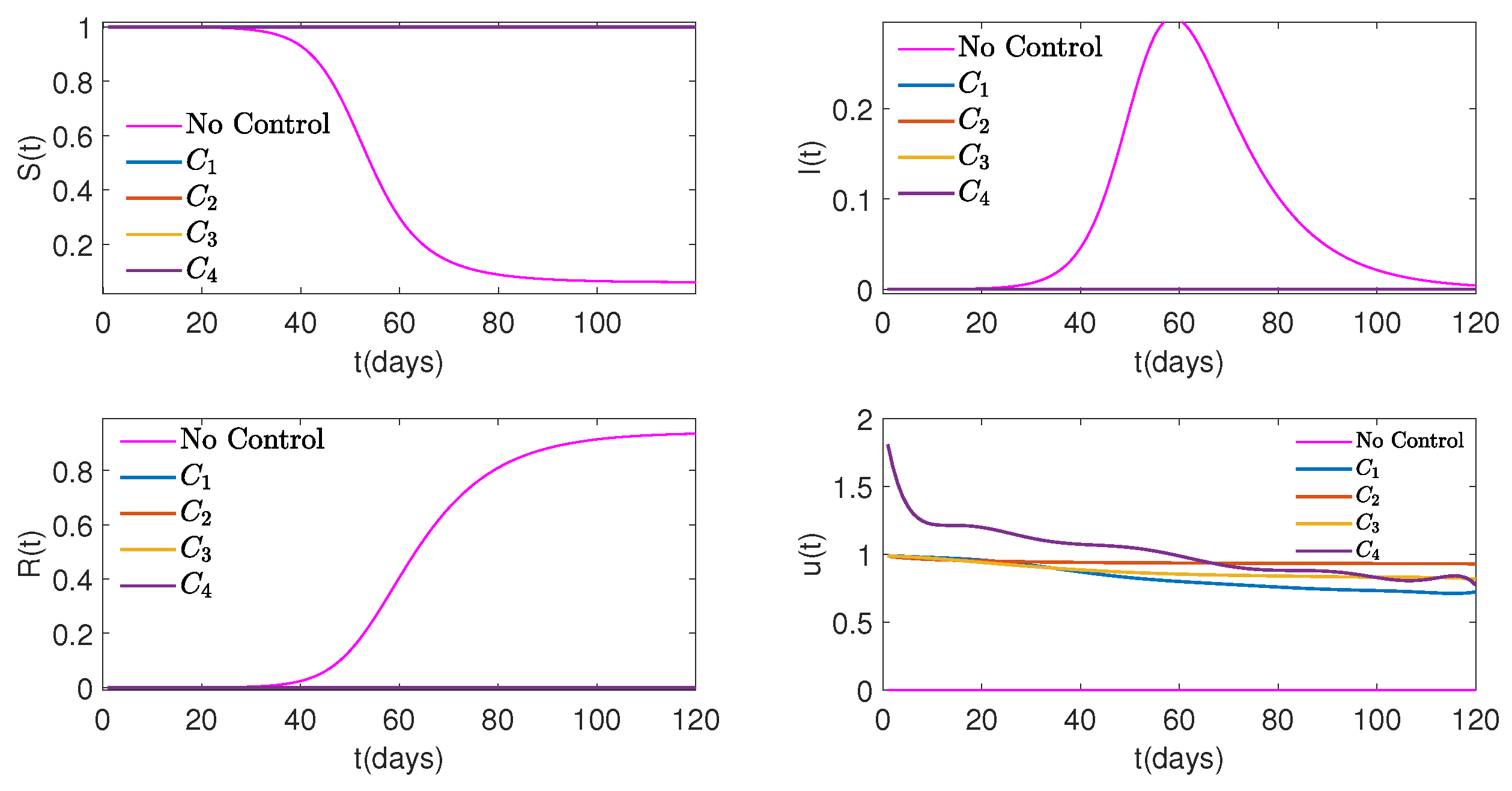
For the next set of experiments, it was assumed that there is only control u 2 ( t ) in the system. In Figure 5, Figure 6, Figure 7, one can see the effect of the weight, λ 2 , on different cost functions and, as the result, on state variables S ( t ) , I ( t ) , and R ( t ) over time. Again, as the weight, λ 2 , decreases the control plays a more effective role in reducing the number of infected people (See Table 2, Table A16, Table A17, and Table A18 for more details).
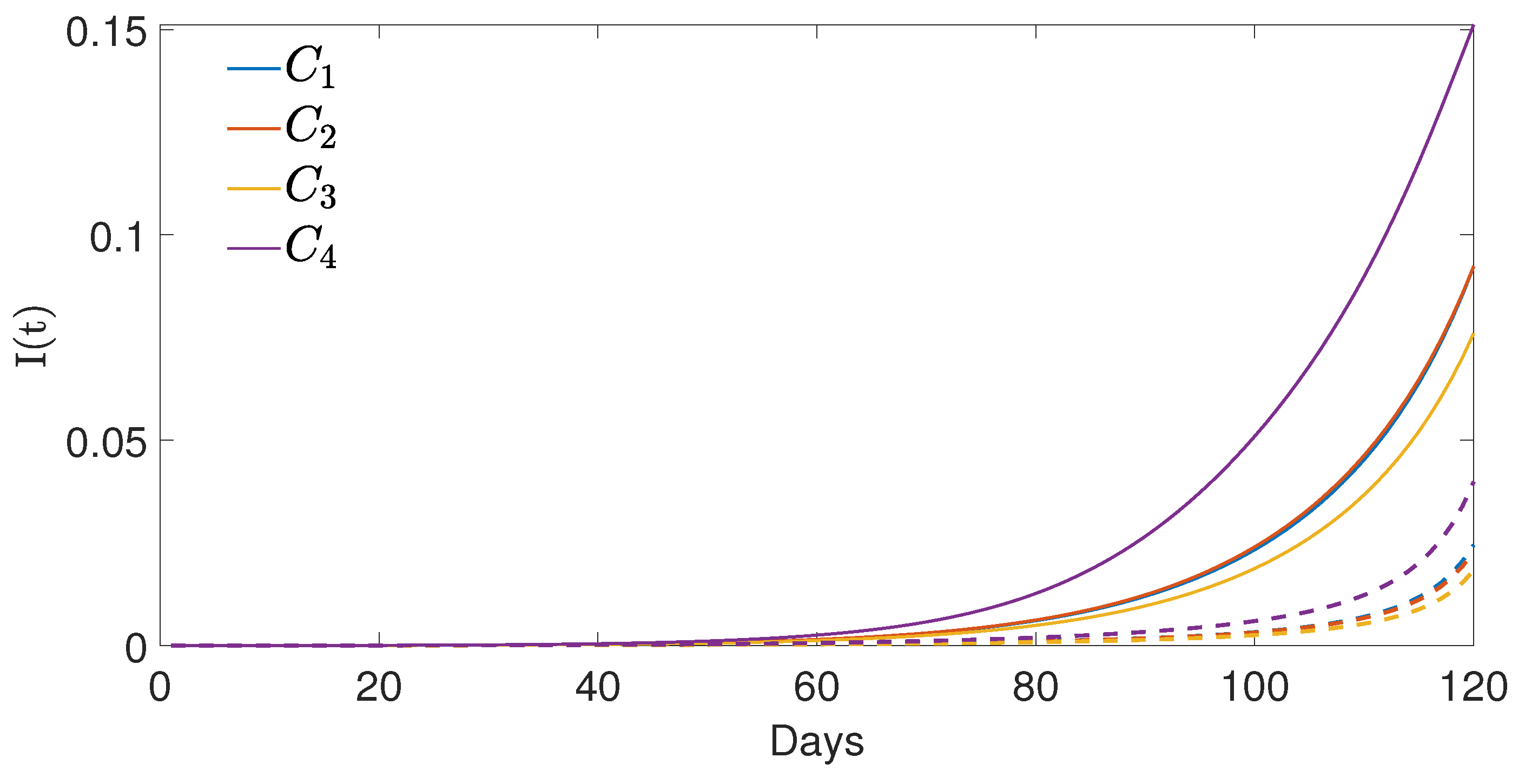
Overall, the effects of controls u 1 ( t ) and u 2 ( t ) on the system, when only one control is applied, are similar. However, as one can clearly see from Table 3, for the same cost and over the same time interval, control u 2 ( t ) suppresses infections more aggressively than u 1 ( t ) . Also, there is a significant difference between the results for cost function C 4 ( u ) and the rest of the cost functions. While for C 1 ( u ) , C 2 ( u ) , and C 3 ( u ) the maximum number of infected people on any given day in the case of "first control only" is 923 , 332 , this number is 1 , 511 , 537 for C 4 ( u ) . Additionally, in the case of "second control only", the maximum daily number of infected individuals for C 4 ( u ) exceeds the maximum daily number for other cost functions by 154 , 151 cases. The best performance among all cost functions can be attributed to C 3 ( u ) in both cases where only control u 1 ( t ) or only control u 2 ( t ) is applied. For details, one can see Table 3 and Figure 8.

4.3. Scenario 3: Non-Medical and Medical Controls in Combination

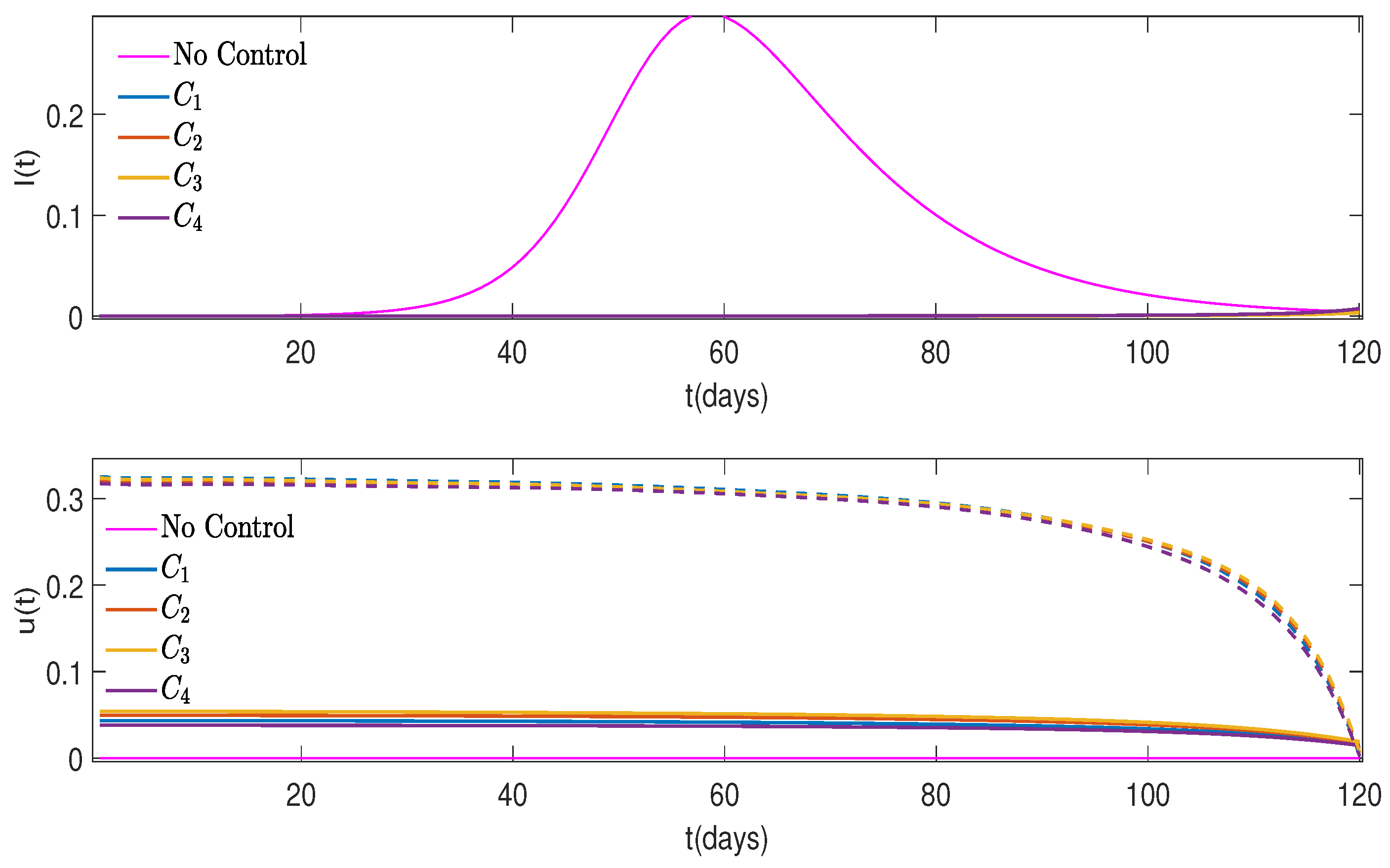
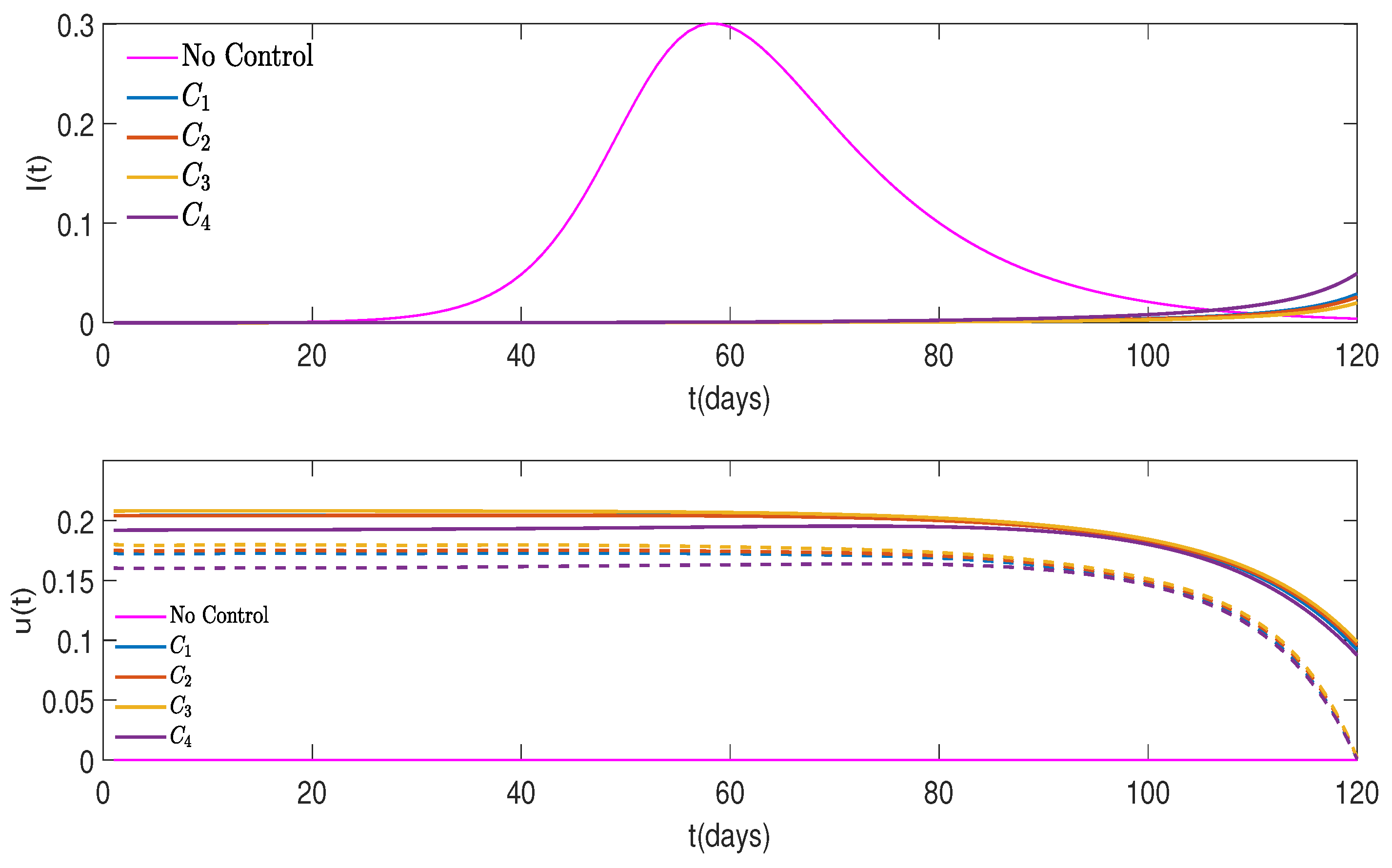
For the next step, we apply two controls to the S I R system, u 1 ( t ) and u 2 ( t ) , together with the same weights, λ 1 = λ 2 = λ , in order to evaluate their effect on the outbreak (See Figure 9, Figure 10, and Figure 11). As expected, in terms of its dependence on λ , the combination of two controls, u 1 ( t ) and u 2 ( t ) , behaves pretty similar to the case of one control in a sense that when the weight, λ , decreases, the controls become more effective, and the daily number of infected humans goes down.
Table 4 and Table 5 show the daily number of infected individuals, I ( t ) , and the cumulative number of infected individuals up to day t, N S ( t ) , for different control scenarios. This gives an insight into how the two controls, u 1 ( t ) and u 2 ( t ) , compare individually and in combination subject to the same cost, C 1 ( u ) , and the same weight, λ 1 = λ 2 = λ = 0.05 .
Table 5 illustrates that the cumulative number of infections after applying both controls for 120 days is 454 , 205 , while the "no control" counterpart is 9 , 397 , 865 . And in the case of control with antiviral medication, u 2 ( t ) , after 120 days there are more than 3 times fewer cases as compared to the case of social distancing control, u 1 ( t ) ( 692 , 160 vs. 2 , 256 , 854 ). Similar tables related to the cost functions C 2 ( u ) , C 3 ( u ) , and C 4 ( u ) can be found in Appendix (Table A1 - Table A6).
In the next series of experiments, controls u 1 ( t ) and u 2 ( t ) have different weights, λ 1 and λ 2 , applied to their respective cost functions. We consider two cases. First, for the cost function C 1 ( u ) , the weight of control u 1 ( t ) is less than the weight of control u 2 ( t ) ( λ 1 < λ 2 ). Table 6 shows changes in daily numbers of infected people, I ( t ) , for the cost function C 1 ( u ) , in the case of fixed weight ( λ 1 = 0.05 ) for control u 1 ( t ) and different weights for control u 2 ( t ) (Table A7 - Table A9 for cost functions C 2 ( u ) , C 3 ( u ) , and C 4 ( u ) can be found in Appendix). As it follows from Table 6, adding the second control, u 2 ( t ) , with any weight, λ 2 , helps to better contain the outbreak and to decrease the daily number of infected people and the cumulative number of cases. Even for high effort case of λ 2 = 0.1 , the number of daily infections is 624 , 040 cases less than the daily number of infected individuals in case when there is no control u 2 ( t ) . However, when the weight of the second control, λ 2 , increases, the effort required to implement that measure also rises, making it increasingly challenging to execute.
If the roles are reversed, that is, for the cost function C 1 ( u ) , the weight, λ 2 = 0.05 , of the second control, u 2 ( t ) , is fixed and the sensitivity of the system to the first control, u 1 ( t ) , is observed, the pattern is similar. Namely, adding a non-medical control, u 1 ( t ) , reduces the daily number of infected people. Even though it is not as consequential as in the case when control u 2 ( t ) is added, still there are fewer infected people in all cases with two controls as opposed to the case of u 2 ( t ) only. At the same time, it is evident that the second control, u 2 ( t ) , is more efficient. Indeed, for the high effort case of λ 1 = 0.1 , the number of daily infections is only 44 , 983 cases less than the daily number of infected individuals in case when there is no control u 1 ( t ) (as opposed to 624 , 040 reduction when u 2 ( t ) was added with the same effort, 0.1 ). The difference in the daily number of infected individuals between the case of no u 1 ( t ) (i.e., u 2 ( t ) only with weight λ 1 = 0.05 ) and the case of u 2 ( t ) with λ 1 = 0.05 and u 1 ( t ) with varying weights ranges from 244 , 998 to 16 , 608 . See Table 7, Table A10, Table A11, and Table A12 for more details.
Figure 13 and Figure 14 show the behavior of controls and their effect on the graphs of I ( t ) for different cost functions and different weights. As it is evident from the graphs, when λ 1 = 0.05 and λ 2 = 0.01 , the second control, u 2 ( t ) , is dominant and very efficient. At the same time, when λ 1 = 0.05 and λ 2 = 0.1 , the two controls, u 1 ( t ) and u 2 ( t ) , are about the same, and there are more infected people towards the end of the study period, that is, the control strategy in Figure 14 is less efficient as compared to the case of Figure 13. The two figures, once again, underline the significance of the second control, u 2 ( t ) .

5. Conclusion

To summarize, in this study, we investigated different control scenarios through theoretical analysis and numerical simulations. To account for two important types of control, social distancing and treatment with antiviral medications, the S I R (Susceptible-Infectious-Removed) model [17] for an early ascending stage of an outbreak has been considered with the first control, u 1 ( t ) , aimed to lower the disease transmission rate and the second control, u 2 ( t ) , aimed to lower the period of infectiousness. In all experiments, the implementation of control strategies reduced the daily cumulative number of cases, N S ( t ) , and successfully "flattened the curve", I ( t ) . The reduction in the cumulative cases was achieved by eliminating or delaying new cases. This delay is incredibly valuable as it provides public health organizations and researchers with more time to advance antiviral treatments and devise alternative preventive measures.
The main theoretical result of this paper, Theorem 3.1, concludes that the optimal control functions, u i ( t ) , i = 1 , 2 , may be increasing until some moment τ [ 0 , T ) . However, for all t [ τ , T ] , the derivatives, d u i d t , become negative and u i ( t ) decline as t approaches T (possibly causing the number of newly infected people to grow). Numerical simulations presented in Section 4 confirm our theoretical findings. So, ideally, around the time t = τ , the control strategy has to be upgraded and a vaccination campaign needs to start to ensure the epidemic wave does not rebound.

Appendix A. Appendix

Appendix A.1. Properties of SIR Model with Time-Dependent Coefficients

In Section 3, it has been pointed out that even though for system (2), the effective reproduction number, r ( t ) = β ( 1 u 1 ( t ) ) / ( γ + ε u 2 ( t ) ) , goes down with more control, it does not guarantee that r ( t ) r ¯ ( t ) yields S ( t ) S ¯ ( t ) for every value of t. One can, however, show that if r ( t ) r ¯ ( t ) and r ( t ) is non-increasing, then S ( t ) S ¯ ( t ) . The proof of this result is given below.
Theorem A.1 Assume that d x d t = f ( x , β , γ ) , x ( 0 ) = x 0 , where x ( t ) = [ S ( t ) , I ( t ) , R ( t ) ] ,
f 1 ( x , β , γ ) : = β ( t ) S ( t ) I ( t ) f 2 ( x , β , γ ) : = β ( t ) S ( t ) I ( t ) γ ( t ) I ( t ) f 3 ( x , β , γ ) : = γ ( t ) I ( t ) ,
a n d x 0 Δ 2 : = { ( z 1 , z 2 , z 3 ) R 3 : z 1 + z 2 + z 3 = 1 , z 1 , z 2 , z 3 0 } .
Let x ( t ) and x ^ ( t ) satisfy d x d t = f ( x , β , γ ) and d x ^ d t = f ( x ^ , β ^ , γ ^ ) , respectively, with the same initial condition x 0 = x ^ 0 = [ S 0 , I 0 , R 0 ] , R 0 0 , S 0 , I 0 > 0 , β ( t ) , γ ( t ) , β ^ ( t ) , γ ^ ( t ) > 0 for any t [ 0 , T ] , and β ( 0 ) > β ^ ( 0 ) > 0 . Suppose r ( t ) : = β ( t ) / γ ( t ) , r ^ ( t ) : = β ^ ( t ) / γ ^ ( t ) , and r ( t ) r ^ ( t ) for all t [ 0 , T ] . If r ( t ) L 1 [ 0 , T ] and r ( t ) is non-increasing, then S ( t ) S ^ ( t ) for any t [ 0 , T ] .
Proof. Since x 0 = x ^ 0 , S 0 , I 0 > 0 and β ( 0 ) > β ^ ( 0 ) , one concludes that S 0 = S ^ 0 > 0 , I 0 = I ^ 0 > 0 , and β ( 0 ) S 0 I 0 > β ^ ( 0 ) S ^ 0 I ^ 0 . Therefore by (A1), S ( 0 ) < S ^ ( 0 ) and there exists ϵ > 0 such that S ( t ) < S ^ ( t ) for any t ( 0 , ϵ ] . If the claim does not hold, then there is μ > ϵ such that S ( μ ) > S ^ ( μ ) . By intermediate value theorem, there exists τ ( ϵ , μ ) such that
S ( t ) < S ^ ( t ) for   any t ( 0 , τ ) S ( τ ) = S ^ ( τ ) and S ( τ ) S ^ ( τ ) .
From (A3), one obtains
S ( τ ) = β ( τ ) S ( τ ) I ( τ ) > β ^ ( τ ) S ^ ( τ ) I ^ ( τ ) = S ( τ ) ,
that is,
I ( τ ) I ^ ( τ ) .
On the other hand, according to (A2)
I ( τ ) I ^ ( τ ) = 1 S ( τ ) R ( τ ) ( 1 S ^ ( τ ) R ^ ( τ ) ) = R ^ ( τ ) R ( τ ) .
As it follows from (A1),
( ln S ( t ) ) = β ( t ) I ( t ) = β ( t ) γ ( t ) R ( t ) = r ( t ) R ( t ) .
This yields,
R ( τ ) = R 0 + 0 τ R ( t ) d t = R 0 0 τ ( ln S ( t ) ) r ( t ) d t .
Identities (A7) and (A8) imply,
I ( τ ) I ^ ( τ ) = 0 τ ( ln S ( t ) ) r ( t ) ( ln S ^ ( t ) ) r ^ ( t ) d t = 0 τ ( ln S ( t ) ) ( ln S ^ ( t ) ) r ( t ) d t = 0 τ 1 r ( t ) 1 r ^ ( t ) ( ln S ^ ( t ) ) d t : = T 1 + T 2 .
Since r ( t ) L 1 [ 0 , T ] is non-increasing, S ( t ) < S ^ ( t ) for any t ( 0 , τ ) , S ( 0 ) = S ^ ( 0 ) , and S ( τ ) = S ^ ( τ ) , by intermediate value theorem for the first term in (A9), one has
T 1 = 0 τ ( ln S ( t ) ) ( ln S ^ ( t ) ) r ( t ) d t = ln S ( t ) ln S ^ ( t ) r ( t ) 0 τ + 0 τ ln S ( t ) ln S ^ ( t ) r ( t ) r 2 ( t ) d t = r ( ν ) r 2 ( ν ) 0 τ ln S ^ ( t ) ln S ( t ) d t 0 ,
where ν [ 0 , τ ] . Furthermore, by Lemma 2.1, S ( t ) , I ( t ) > 0 and ( ln S ( t ) ) < 0 for any t [ 0 , T ] . Hence from r ( t ) r ^ ( t ) it follows that
T 2 = 0 τ 1 r ( t ) 1 r ^ ( t ) ( ln S ^ ( t ) ) d t = 1 r ( σ ) 1 r ^ ( σ ) 0 τ ( ln S ^ ( t ) ) d t = 1 r ^ ( σ ) 1 r ( σ ) S ^ ( 0 ) S ^ ( τ ) > 0 .
Combining (A10) and (A11), one concludes that I ( τ ) > I ^ ( τ ) , which contradicts (A5). This completes the proof. □

Appendix A.2. Additional Tables

Table A1. Comparison of I ( t ) for cost function C 2 when there is only u 1 , only u 2 , and both u 1 , u 2 applied versus No Control case over time when λ = 0.05 .
Day No Control λ 1 = 0.05             No 2nd Control No 1st Control     λ 2 = 0.05 λ 1 = 0.05 λ 2 = 0.05
1 200 200 200 200
10 1,237 388 317 298
20 9,228 816 527 464
30 67,606 1,706 872 725
40 456,639 3,557 1,439 1,132
50 1,985,292 7,379 2,362 1,765
60 2,987,989 15,209 3,879 2,772
70 2,015,872 31,076 6,381 4,403
80 1,023,788 62,623 10,561 7,122
90 474,813 123,913 17,880 11,975
100 213,085 240,619 32,336 21,814
110 94,393 463,527 67,697 46,675
120 41,578 923,332 229,683 156,190
Table A2. Comparison of I ( t ) for cost function C 3 when there is only u 1 , only u 2 , and both u 1 , u 2 applied versus No Control case over time when λ = 0.05 .
Day No Control λ 1 = 0.05             No 2nd Control No 1st Control     λ 2 = 0.05 λ 1 = 0.05 λ 2 = 0.05
1 200 200 200 200
10 1,237 377 308 289
20 9,228 766 495 437
30 67,606 1,552 795 662
40 456,639 3,134 1,273 1,003
50 1,985,292 6,302 2,034 1,524
60 2,987,989 12,618 3,258 2,333
70 2,015,872 25,120 5,256 3,624
80 1,023,788 49,586 8,558 5,751
90 474,813 96,926 14,338 9,523
100 213,085 188,180 25,768 17,140
110 94,393 367,745 53,756 36,352
120 41,578 760,101 183,048 121,390
Table A3. Comparison of I ( t ) for cost function C 4 when there is only u 1 , only u 2 , and both u 1 , u 2 applied versus No Control case over time when λ = 0.05 .
Day No Control λ 1 = 0.05             No 2nd Control No 1st Control     λ 2 = 0.05 λ 1 = 0.05 λ 2 = 0.05
1 200 200 200 200
10 1,237 417 349 323
20 9,228 942 644 550
30 67,606 2,150 1,178 935
40 456,639 4,890 2,133 1,581
50 1,985,292 11,061 3,816 2,663
60 2,987,989 24,982 6,733 4,478
70 2,015,872 55,154 11,672 7,537
80 1,023,788 113,747 19,877 12,760
90 474,813 214,937 33,825 22,145
100 213,085 393,864 60,100 41,039
110 94,393 765,135 123,379 88,776
120 41,578 1,493,486 399,149 292,220
Table A4. Cumulative number of infections up to day t, N S ( t ) for cost function C 2 when there is only u 1 , only u 2 , and both u 1 , u 2 versus No Control case over time when weight λ 1 = λ 2 = λ = 0.05 .
Day No Control λ 1 = 0.05         No 2nd Control No 1st Control    λ 2 = 0.05 λ 1 = 0.05 λ 2 = 0.05
1 200 200 200 200
10 1,756 644 897 767
20 13,747 1,657 2,149 1,738
30 101,568 3,762 4,215 3,249
40 697,572 8,148 7,626 5,604
50 3,338,392 17,229 13,223 9,267
60 7,032,920 35,913 22,418 15,000
70 8,627,485 74,051 37,492 24,055
80 9,121,747 150,774 62,328 38,584
90 9,292,217 302,212 103,637 62,591
100 9,358,556 595,429 175,436 104,787
110 9,386,082 1,158,900 313,167 188,825
120 9,397,865 2,283,654 665,799 416,713
Table A5. Cumulative number of infections up to day t, N S ( t ) for cost function C 3 when there is only u 1 , only u 2 , and both u 1 , u 2 versus No Control case over time when weight λ 1 = λ 2 = λ = 0.05 .
Day No Control λ 1 = 0.05         No 2nd Control No 1st Control    λ 2 = 0.05 λ 1 = 0.05 λ 2 = 0.05
1 200 200 200 200
10 1,756 629 885 754
20 13,747 1,575 2,078 1,677
30 101,568 3,482 3,988 3,067
40 697,572 7,331 7,047 5,170
50 3,338,392 15,051 11,930 8,358
60 7,032,920 30,487 19,736 13,210
70 8,627,485 61,195 32,284 20,701
80 9,121,747 121,742 52,562 32,483
90 9,292,217 239,921 85,884 51,635
100 9,358,556 469,095 143,369 84,866
110 9,386,082 916,823 253,443 150,547
120 9,397,865 1,846,297 536,094 328,156
Table A6. Cumulative number of infections up to day t, N S ( t ) for cost function C 4 when there is only u 1 , only u 2 , and both u 1 , u 2 versus No Control case over time when weight λ 1 = λ 2 = λ = 0.05 .
Day No Control λ 1 = 0.05         No 2nd Control No 1st Control    λ 2 = 0.05 λ 1 = 0.05 λ 2 = 0.05
1 200 200 200 200
10 1,756 685 937 803
20 13,747 1,863 2,398 1,927
30 101,568 4,545 5,068 3,835
40 697,572 10,636 9,909 7,055
50 3,338,392 24,388 18,614 12,483
60 7,032,920 55,445 34,055 21,602
70 8,627,485 123,916 60,931 36,924
80 9,121,747 264,191 106,859 62,740
90 9,292,217 525,613 184,436 106,949
100 9,358,556 1,000,085 317,429 186,138
110 9,386,082 1,928,590 565,198 344,961
120 9,397,865 3,757,435 1,169,728 768,757
Table A7. Comparison of the daily number of infected people, I ( t ) , for the cost function C 2 with the weight λ 1 = 0.05 for u 1 ( t ) . The weights for the control u 2 ( t ) are λ 2 = 0.001 , 0.01 , 0.05 , and 0.1 for the second, third, and fourth columns, respectively, and the fifth column shows the case of No Control u 2 ( t ) over time.
Day λ 1 = 0.05 λ 2 = 0.001 λ 1 = 0.05 λ 2 = 0.01 λ 1 = 0.05 λ 2 = 0.05 λ 1 = 0.05 λ 2 = 0.1 λ 1 = 0.05        No 2nd Control
1 200 200 200 200 200
10 183 251 298 317 388
20 171 324 464 532 816
30 168 422 725 892 1,706
40 171 556 1,132 1,490 3,557
50 182 740 1,765 2,483 7,379
60 203 1,006 2,772 4,143 15,209
70 240 1,408 4,403 6,949 31,076
80 302 2,046 7,122 11,770 62,623
90 415 3,162 11,975 20,464 123,913
100 656 5,454 21,814 37,902 240,619
110 1,290 11,440 46,675 80,593 463,527
120 4,634 41,179 156,190 251,157 923,332
Table A8. Comparison of the daily number of infected people, I ( t ) , for the cost function C 3 with the weight λ 1 = 0.05 for u 1 ( t ) . The weights for the control u 2 ( t ) are λ 2 = 0.001 , 0.01 , 0.05 , and 0.1 for the second, third, and fourth columns, respectively, and the fifth column shows the case of No Control u 2 ( t ) over time.
Day λ 1 = 0.05 λ 2 = 0.001 λ 1 = 0.05 λ 2 = 0.01 λ 1 = 0.05 λ 2 = 0.05 λ 1 = 0.05 λ 2 = 0.1 λ 1 = 0.05        No 2nd Control
1 200 200 200 200 200
10 179 245 289 308 377
20 165 309 437 498 766
30 160 394 662 807 1,552
40 161 508 1,003 1,305 3,134
50 168 662 1,524 2,107 6,302
60 185 884 2,333 3,416 12,618
70 216 1,217 3,624 5,586 25,120
80 267 1,739 5,751 9,264 49,586
90 361 2,647 9,523 15,856 96,926
100 560 4,497 17,140 29,108 188,180
110 1,074 9,247 36,352 61,700 367,745
120 3,747 32,698 121,390 194,169 760,101
Table A9. Comparison of the daily number of infected people, I ( t ) , for the cost function C 4 with the weight λ 1 = 0.05 for u 1 ( t ) . The weights for the control u 2 ( t ) are λ 2 = 0.001 , 0.01 , 0.05 , and 0.1 for the second, third, and fourth columns, respectively, and the fifth column shows the case of No Control u 2 ( t ) over time.
Day λ 1 = 0.05 λ 2 = 0.001 λ 1 = 0.05 λ 2 = 0.01 λ 1 = 0.05 λ 2 = 0.05 λ 1 = 0.05 λ 2 = 0.1 λ 1 = 0.05        No 2nd Control
1 200 200 200 200 200
10 185 263 323 351 401
20 177 357 550 658 918
30 177 490 935 1,227 2,133
40 185 675 1,581 2,274 4,939
50 202 937 2,663 4,178 11,366
60 232 1,326 4,478 7,610 25,851
70 284 1,929 7,537 13,717 57,953
80 373 2,911 12,760 24,464 127,302
90 540 4,681 22,145 43,673 266,304
100 907 8,432 41,039 80,621 509,874
110 1,955 18,778 88,776 166,824 899,275
120 7,639 71,495 292,220 482,565 1,511,537
Table A10. Comparison of the daily number of infected people, I ( t ) , for the cost function C 2 with the weight λ 2 = 0.05 for u 2 ( t ) . The weights for the control u 1 ( t ) are λ 1 = 0.001 , 0.01 , 0.05 , and 0.1 for the second, third, and fourth columns, respectively, and the fifth column shows the case of No Control u 1 ( t ) over time.
Day λ 1 = 0.001 λ 2 = 0.05 λ 1 = 0.01 λ 2 = 0.05 λ 1 = 0.05 λ 2 = 0.05 λ 1 = 0.1 λ 2 = 0.05 No 1st Control λ 2 = 0.05
1 200 200 200 200 200
10 244 279 298 304 317
20 308 406 464 485 527
30 391 593 725 773 872
40 501 869 1,132 1,232 1,439
50 650 1,280 1,765 1,957 2,362
60 859 1,908 2,772 3,124 3,879
70 1,163 2,896 4,403 5,028 6,381
80 1,628 4,517 7,122 8,203 10,561
90 2,393 7,382 11,975 13,833 17,880
100 3,793 13,124 21,814 25,193 32,336
110 6,858 27,281 46,675 53,697 67,697
120 16,447 82,599 156,190 181,647 229,683
Table A11. Comparison of the daily number of infected people, I ( t ) , for the cost function C 3 with the weight λ 2 = 0.05 for u 2 ( t ) . The weights for the control u 1 ( t ) are λ 1 = 0.001 , 0.01 , 0.05 , and 0.1 for the second, third, and fourth columns, respectively, and the fifth column shows the case of No Control u 1 ( t ) over time.
Day λ 1 = 0.001 λ 2 = 0.05 λ 1 = 0.01 λ 2 = 0.05 λ 1 = 0.05 λ 2 = 0.05 λ 1 = 0.1 λ 2 = 0.05 No 1st Control λ 2 = 0.05
1 200 200 200 200 200
10 241 274 289 295 308
20 299 388 437 456 495
30 375 546 662 705 795
40 475 772 1,003 1,090 1,273
50 609 1,116 1,524 1,682 2,034
60 795 1,636 2,333 2,617 3,258
70 1,065 2,421 3,624 4,119 5,256
80 1,473 3,676 5,751 6,596 8,558
90 2,138 5,900 9,523 10,976 14,338
100 3,349 10,387 17,140 19,806 25,768
110 5,944 21,561 36,352 41,897 53,756
120 13,985 65,461 121,390 141,870 183,048
Table A12. Comparison of the daily number of infected people, I ( t ) , for the cost function C 4 with the weight λ 2 = 0.05 for u 2 ( t ) . The weights for the control u 1 ( t ) are λ 1 = 0.001 , 0.01 , 0.05 , and 0.1 for the second, third, and fourth columns, respectively, and the fifth column shows the case of No Control u 1 ( t ) over time.
Day λ 1 = 0.001 λ 2 = 0.05 λ 1 = 0.01 λ 2 = 0.05 λ 1 = 0.05 λ 2 = 0.05 λ 1 = 0.1 λ 2 = 0.05 No 1st Control λ 2 = 0.05
1 200 200 200 200 200
10 243 295 323 331 349
20 305 458 550 581 644
30 386 711 935 1,016 1,178
40 493 1,105 1,581 1,765 2,133
50 642 1,723 2,663 3,040 3,816
60 857 2,705 4,478 5,206 6,733
70 1,181 4,303 7,537 8,876 11,672
80 1,688 7,008 12,760 15,100 19,877
90 2,559 11,918 22,145 26,079 33,825
100 4,271 21,947 41,039 47,785 60,100
110 8,353 47,241 88,776 101,665 123,379
120 22,600 146,614 292,220 334,465 399,149
Table A13. Comparison of I ( t ) for cost function C 2 in case when only control u 1 is applied and λ 1 varies. As λ 1 increases, the number of infected individuals, I ( t ) , gets higher on most days.
Day λ 1 = 10 7      No 2nd Control λ 1 = 0.001 No 2nd Control λ 1 = 0.01 No 2nd Control λ 1 = 0.05 No 2nd Control No Control
1 200 200 200 200 200
10 88 255 317 388 1,237
20 36 334 533 816 9,228
30 15 441 894 1,706 67,606
40 6 586 1,498 3,557 456,639
50 3 786 2,512 7,379 1,985,292
60 1 1,068 4,219 15,209 2,987,989
70 0 1,479 7,126 31,076 2,015,872
80 0 2,101 12,151 62,623 1,023,788
90 0 3,105 21,130 123,913 474,813
100 0 4,883 38,221 240,619 213,085
110 0 8,576 74,708 463,527 94,393
120 0 19,158 177,113 923,332 41,578
Table A14. Comparison of I ( t ) for cost function C 3 in case when only control u 1 is applied and λ 1 varies. As λ 1 increases, the number of infected individuals, I ( t ) , gets higher on most days.
Day λ 1 = 10 7      No 2nd Control λ 1 = 0.001 No 2nd Control λ 1 = 0.01 No 2nd Control λ 1 = 0.05 No 2nd Control No Control
1 200 200 200 200 200
10 86 254 314 377 1,237
20 35 332 522 766 9,228
30 15 437 867 1,552 67,606
40 8 579 1,438 3,134 456,639
50 4 773 2,388 6,302 1,985,292
60 2 1,044 3,972 12,618 2,987,989
70 1 1,437 6,644 25,120 2,015,872
80 1 2,025 11,220 49,586 1,023,788
90 0 2,963 19,303 96,926 474,813
100 0 4,592 34,478 188,180 213,085
110 0 7,879 66,265 367,745 94,393
120 0 16,955 153,051 760,101 41,578
Table A15. Comparison of I ( t ) for cost function C 4 in case when only control u 1 is applied and λ 1 varies. As λ 1 increases, the number of infected individuals, I ( t ) , gets higher on most days.
Day λ 1 = 10 7      No 2nd Control λ 1 = 0.001 No 2nd Control λ 1 = 0.01 No 2nd Control λ 1 = 0.05 No 2nd Control No Control
1 200 200 200 200 200
10 28 248 319 401 1,237
20 4 315 542 918 9,228
30 1 405 917 2,133 67,606
40 0 527 1,550 4,939 456,639
50 0 696 2,623 11,366 1,985,292
60 0 936 4,447 25,851 2,987,989
70 0 1,296 7,593 57,953 2,015,872
80 0 1,865 13,135 127,302 1,023,788
90 0 2,840 23,348 266,304 474,813
100 0 4,726 43,733 509,874 213,085
110 0 9,137 91,108 899,275 94,393
120 0 24,025 240,585 1,511,537 41,578
Table A16. Comparison of I ( t ) for cost function C 2 in case when only control u 2 is applied and λ 2 varies. As λ 2 increases, the number of infected individuals, I ( t ) , gets higher on most days.
Day λ 2 = 10 7        No 1st Control λ 2 = 0.001   No 1st Control λ 2 = 0.01   No 1st Control λ 2 = 0.05   No 1st Control λ 2 = 0.1   No 1st Control No Control
1 200 200 200 200 200 200
10 17 183 255 317 369 1,237
20 1 172 335 527 722 9,228
30 0 169 444 872 1,404 67,606
40 0 173 592 1,439 2,701 456,639
50 0 185 797 2,362 5,115 1,985,292
60 0 207 1,095 3,879 9,510 2,987,989
70 0 245 1,546 6,381 17,215 2,015,872
80 0 311 2,267 10,561 30,078 1,023,788
90 0 437 3,527 17,880 51,136 474,813
100 0 695 6,103 32,336 87,648 213,085
110 0 1,398 12,821 67,697 164,273 94,393
120 0 5,103 46,967 229,683 464,307 41,578
Table A17. Comparison of I ( t ) for cost function C 3 in case when only control u 2 is applied and λ 2 varies. As λ 2 increases, the number of infected individuals, I ( t ) , gets higher on most days.
Day λ 2 = 10 7        No 1st Control λ 2 = 0.001   No 1st Control λ 2 = 0.01   No 1st Control λ 2 = 0.05   No 1st Control λ 2 = 0.1   No 1st Control No Control
1 200 200 200 200 200 200
10 17 180 250 308 347 1,237
20 1 166 321 495 636 9,228
30 0 161 417 795 1,159 67,606
40 0 163 546 1,273 2,096 456,639
50 0 171 723 2,034 3,752 1,985,292
60 0 189 978 3,258 6,656 2,987,989
70 0 219 1,359 5,256 11,661 2,015,872
80 0 274 1,962 8,558 20,100 1,023,788
90 0 377 3,014 14,338 34,531 474,813
100 0 587 5,134 25,768 61,227 213,085
110 0 1,147 10,559 53,756 120,600 94,393
120 0 4,067 37,929 183,048 365,469 41,578
Table A18. Comparison of I ( t ) for cost function C 4 in case when only control u 2 is applied and λ 2 varies. As λ 2 increases, the number of infected individuals, I ( t ) , gets higher on most days.
Day λ 2 = 10 7        No 1st Control λ 2 = 0.001   No 1st Control λ 2 = 0.01   No 1st Control λ 2 = 0.05   No 1st Control λ 2 = 0.1   No 1st Control No Control
1 200 200 200 200 200 200
10 2 185 265 349 381 1,237
20 0 177 364 644 767 9,228
30 0 177 501 1,178 1,531 67,606
40 0 186 695 2,133 3,019 456,639
50 0 204 972 3,816 5,908 1,985,292
60 0 235 1,384 6,733 11,591 2,987,989
70 0 288 2,021 11,672 22,889 2,015,872
80 0 382 3,067 19,877 45,018 1,023,788
90 1 559 4,960 33,825 86,814 474,813
100 1 949 8,995 60,100 165,937 213,085
110 0 2,069 20,200 123,379 338,415 94,393
120 0 8,174 78,701 399,149 878,072 41,578

References

  1. Cai, L.; Li, X.; Tuncer, N.; Martcheva, M.; Lashari, A.A. Optimal control of a malaria model with asymptomatic class and superinfection. Mathematical Biosciences 2017, 288, 94–108. [Google Scholar] [CrossRef] [PubMed]
  2. Panovska-Griffiths, J.; Kerr, C.C.; Stuart, R.M.; Mistry, D.; Klein, D.J.; Viner, R.M.; Bonell, C. Determining the optimal strategy for reopening schools, the impact of test and trace interventions, and the risk of occurrence of a second COVID-19 epidemic wave in the UK: a modelling study. The Lancet Child & Adolescent Health 2020, 4, 817–827. [Google Scholar]
  3. Paltiel, A.D.; Zheng, A.; Walensky, R.P. Assessment of SARS-CoV-2 screening strategies to permit the safe reopening of college campuses in the United States. JAMA network open 2020, 3, e2016818–e2016818. [Google Scholar] [CrossRef] [PubMed]
  4. Aaby, P.; Samb, B.; Simondon, F.; Seck, A.M.C.; Knudsen, K.; Whittle, H. Non-specific beneficial effect of measles immunisation: analysis of mortality studies from developing countries. Bmj 1995, 311, 481–485. [Google Scholar] [CrossRef] [PubMed]
  5. Ahmed, F.; Lindley, M.C.; Allred, N.; Weinbaum, C.M.; Grohskopf, L. Effect of influenza vaccination of healthcare personnel on morbidity and mortality among patients: systematic review and grading of evidence. Clinical infectious diseases 2014, 58, 50–57. [Google Scholar] [CrossRef] [PubMed]
  6. Sivaraman, K.; Dhawan, S.; Chopra, A.; Bhat, S.G. How Effective Were Isolation and Quarantine Strategies during the COVID-19 Pandemic: Challenges and Lessons Learned So Far? Preprints.org 2024. [Google Scholar]
  7. Strassburg, M.A. The global eradication of smallpox. American journal of infection control 1982, 10, 53–59. [Google Scholar] [CrossRef] [PubMed]
  8. D’Ortenzio, E.; Do, C.; Renault, P.; Weber, F.; Filleul, L. Enhanced influenza surveillance on Réunion Island (southern hemisphere) in the context of the emergence of influenza A(H1N1)v. Eurosurveillance 2009, 14, 19239. [Google Scholar] [CrossRef] [PubMed]
  9. Barlow M., M. N.; R., T. Optimal shutdown strategies for COVID-19 with economic and mortality costs: British Columbia as a case study. Royal Society Open Science 2021, 8, 1–18. [Google Scholar] [CrossRef] [PubMed]
  10. Saha, S.; Samanta, G. Modelling the role of optimal social distancing on disease prevalence of COVID-19 epidemic. International Journal of Dynamics and Control 2021, 9, 1053–1077. [Google Scholar] [CrossRef] [PubMed]
  11. Saha, S.; Samanta, G.; Nieto, J. Impact of optimal vaccination and social distancing on COVID-19 pandemic. Mathematics and Computers in Simulation 2022, 200, 285–314. [Google Scholar] [CrossRef] [PubMed]
  12. Firth, J.A.; Hellewell, J.; Klepac, P.; Kissler, S.; Kucharski, A.J.; Spurgin, L.G. Using a real-world network to model localized COVID-19 control strategies. Nature medicine 2020, 26, 1616–1622. [Google Scholar] [CrossRef] [PubMed]
  13. Köhler, J.; Schwenkel, L.; Koch, A.; Berberich, J.; Pauli, P.; Allgöwer, F. Robust and optimal predictive control of the COVID-19 outbreak. Annual Reviews in Control 2021, 51, 525–539. [Google Scholar] [CrossRef] [PubMed]
  14. Lü, X.; Hui, H.w.; Liu, F.f.; Bai, Y.l. Stability and optimal control strategies for a novel epidemic model of COVID-19. Nonlinear Dynamics 2021, 106, 1491–1507. [Google Scholar] [CrossRef] [PubMed]
  15. Tuncer, N.; Timsina, A.; Nuno, M.; Chowell, G.; Martcheva, M. Parameter identifiability and optimal control of an SARS-CoV-2 model early in the pandemic. Journal of Biological Dynamics 2022, 16, 412–438. [Google Scholar] [CrossRef] [PubMed]
  16. Ghosh, J.K.; Ghosh, U.; Biswas, M.; Sarkar, S. Qualitative analysis and optimal control strategy of an SIR model with saturated incidence and treatment. Differential Equations and Dynamical Systems. [CrossRef]
  17. Kermack, W.O.; McKendrick, A.G. A contribution to the mathematical theory of epidemics. Proceedings of the royal society of london. Series A, Containing papers of a mathematical and physical character 1927, 115, 700–721. [Google Scholar]
  18. Hethcote, H.W.; Yorke, J.A. Gonorrhea transmission dynamics and control; Vol. 56, Springer, 2014.
  19. Lee, S.; Chowell, G.; Castillo-Chávez, C. Optimal control for pandemic influenza: The role of limited antiviral treatment and isolation. Journal of Theoretical Biology 2010, 265, 136–150. [Google Scholar] [CrossRef] [PubMed]
  20. Smirnova, A.; Ye, X. On Optimal Control at the Onset of a New Viral Outbreak. Infectious Disease Modelling 2024. [Google Scholar] [CrossRef] [PubMed]
  21. Lenhart, S. ; J.T.Workman. Optimal control applied to biological models. Chapman and Hall/CRC. [CrossRef]
  22. Pontryagin, L.S. Mathematical Theory of Optimal Processes; Routledge, 2018.
Figure 1. Comparison of the four control cost functions used in numerical experiments below: C 1 ( u ) = 0.830071 ln ( 1 u 2 ) , C 2 ( u ) = 0.672850 u ln ( 1 u ) , C 3 ( u ) = z ln ( 1 u ) , C 4 ( u ) = 1.424546 u 2 .
Preprints 116455 g001
Figure 2. Graphs of Susceptible S ( t ) (top on the left), Infected I ( t ) (top on the right), Recovered R ( t ) (bottom on the left) people, and control u 1 ( t ) (bottom on the right) over time for four different cost functions C 1 , C 2 , C 3 , C 4 versus No Control when weight is λ 1 = 0.05 .
Preprints 116455 g002
Figure 3. Graphs of Susceptible S ( t ) (top on the left), Infected I ( t ) (top on the right), Recovered R ( t ) (bottom on the left) people, and control u 1 ( t ) (bottom on the right) over time for four different cost functions C 1 , C 2 , C 3 , C 4 versus No Control when weight is λ 1 = 0.001 .
Preprints 116455 g003
Figure 4. Graphs of Susceptible S ( t ) (top on the left), Infected I ( t ) (top on the right), Recovered R ( t ) (bottom on the left) people, and control u 1 ( t ) (bottom on the right) over time for four different cost functions C 1 , C 2 , C 3 , C 4 versus No Control when weight is λ 1 = 10 7 . For the cost function C 4 , u 1 ( t ) stays above the ultimate value, u 1 ( t ) = 1 , for more than half of the study period, which is not practical.
Preprints 116455 g004
Figure 5. Graphs of Susceptible S ( t ) (top on the left), Infected I ( t ) (top on the right), Recovered R ( t ) (bottom on the left) people, and control u 2 ( t ) (bottom on the right) over time for four different cost functions C 1 , C 2 , C 3 , C 4 versus No Control when weight is λ = 0.1 .
Preprints 116455 g005
Figure 6. Graphs of Susceptible S ( t ) (top on the left), Infected I ( t ) (top on the right), Recovered R ( t ) (bottom on the left) people, and control u 2 ( t ) (bottom on the right) over time for four different cost functions C 1 , C 2 , C 3 , C 4 versus No Control when weight is λ 2 = 0.05 .
Preprints 116455 g006
Figure 7. Graphs of Susceptible S ( t ) (top on the left), Infected I ( t ) (top on the right), Recovered R ( t ) (bottom on the left) people, and control u 2 ( t ) (bottom on the right) over time for four different cost functions C 1 , C 2 , C 3 , C 4 versus No Control when weight is λ 2 = 10 7 .
Preprints 116455 g007
Figure 8. Graphs of I ( t ) for different cost functions C 1 , C 2 , C 3 , C 4 when only u 1 is applied and λ 1 = 0.05 (shown with solid lines), and when only u 2 is applied and λ 2 = 0.05 (shown with dashed line).
Preprints 116455 g008
Figure 9. Graphs of Susceptible S ( t ) (top on the left), Infected I ( t ) (top on the right), Recovered R ( t ) (bottom on the left) people, and controls u 1 ( t ) shown with solid lines, and u 2 ( t ) with dashed lines (bottom on the right) over time for four different cost functions C 1 , C 2 , C 3 , C 4 versus No Control when weights, λ 1 , and λ 2 , for both controls are 0.1 .
Preprints 116455 g009
Figure 10. Graphs of Susceptible S ( t ) (top on the left), Infected I ( t ) (top on the right), Recovered R ( t ) (bottom on the left) people, and control u 1 shown with solid lines, and u 2 with dashed lines (bottom on the right) over time for four different cost functions C 1 , C 2 , C 3 , C 4 versus No Control when weight, λ , for both controls is λ 1 = λ 2 = λ = 0.05 .
Preprints 116455 g010
Figure 11. Graphs of Susceptible S ( t ) (top on the left), Infected I ( t ) (top on the right), Recovered R ( t ) (bottom on the left) people, and controls u 1 ( t ) shown with solid lines, and u 2 ( t ) with dashed lines (bottom on the right) over time for four different cost functions C 1 , C 2 , C 3 , C 4 versus No Control when weight, λ , for both controls is λ 1 = λ 2 = λ = 0.001 .
Preprints 116455 g011
Figure 12. Graphs of Susceptible S ( t ) (top on the left), Infected I ( t ) (top on the right), Recovered R ( t ) (bottom on the left) people, and controls u 1 ( t ) shown with solid lines and u 2 ( t ) with dashed lines (bottom on the right) for four different cost functions C 1 , C 2 , C 3 , C 4 versus No Control when weight, λ , for both controls is λ 1 = λ 2 = λ = 10 8 . Control u 2 for cost function C 4 takes unrealistic values above 1 at the early period of the study.
Preprints 116455 g012
Figure 13. The proportion of Infected people, I ( t ) , for different cost functions and No Control case when λ 1 = 0.05 , λ 2 = 0.01 (on the top ) and controls u 1 ( t ) shown with solid lines, and u 2 ( t ) with dashed lines (on the bottom).
Preprints 116455 g013
Figure 14. The proportion of Infected people, I ( t ) , for different cost functions and No Control case when λ 1 = 0.05 , λ 2 = 0.1 (on the top) and controls u 1 ( t ) shown with solid lines, and u 2 ( t ) with dashed lines (on the bottom).
Preprints 116455 g014
Table 1. Comparison of I ( t ) for cost function C 1 in case when only control u 1 is applied and λ 1 varies. As λ 1 increases, the number of infected individuals, I ( t ) , gets higher on most days.
Day λ 1 = 10 7      No 2nd Control λ 1 = 0.001 No 2nd Control λ 1 = 0.01 No 2nd Control λ 1 = 0.05 No 2nd Control No Control
1 200 200 200 200 200
10 85 253 315 387 1,237
20 34 329 527 812 9,228
30 15 432 880 1,691 67,606
40 7 571 1,466 3,514 456,639
50 4 761 2,447 7,267 1,985,292
60 3 1,028 4,089 14,927 2,987,989
70 2 1,416 6,873 30,388 2,015,872
80 1 2,003 11,678 61,024 1,023,788
90 1 2,953 20,264 120,429 474,813
100 1 4,643 36,661 233,756 213,085
110 1 8,190 72,008 453,110 94,393
120 1 18,714 174,758 922,708 41,578
Table 2. Comparison of I ( t ) for cost function C 1 in case when only control u 2 is applied and λ 2 varies. As λ 2 increases, the number of infected individuals, I ( t ) , gets higher on most days.
Day λ 2 = 10 7        No 1st Control λ 2 = 0.001   No 1st Control λ 2 = 0.01   No 1st Control λ 2 = 0.05   No 1st Control λ 2 = 0.1   No 1st Control No Control
1 200 200 200 200 200 200
10 18 181 254 318 377 1,237
20 1 168 332 530 756 9,228
30 0 164 437 880 1,503 67,606
40 0 166 581 1,456 2,949 456,639
50 0 177 782 2,395 5,693 1,985,292
60 0 198 1,073 3,938 10,735 2,987,989
70 0 234 1,515 6,481 19,547 2,015,872
80 0 299 2,226 10,735 34,005 1,023,788
90 0 420 3,485 18,210 56,943 474,813
100 0 676 6,092 33,048 95,559 213,085
110 0 1,391 13,102 70,339 177,085 94,393
120 0 5,265 49,724 244,998 499,616 41,578
Table 3. Comparison of I ( t ) for all cost functions in the case when only control u 1 is applied ( λ 1 = 0.05 ) or only control u 2 is applied ( λ 2 = 0.05 ) over time.
Day λ 1 = 0.05            No 2nd Control No 1st Control λ 2 = 0.05 λ 1 = 0.05 No 2nd Control No 1st Control λ 2 = 0.05 λ 1 = 0.05 No 2nd Control No 1st Control λ 2 = 0.05 λ 1 = 0.05 No 2nd Control No 1st Control λ 2 = 0.05
C 1 C 2 C 3 C 4
1 200 200 200 200 200 200 200 200
10 387 318 388 317 377 308 401 349
20 812 530 816 527 766 495 918 644
30 1,691 880 1,706 872 1,552 795 2,133 1,178
40 3,514 1,456 3,557 1,439 3,134 1,273 4,939 2,133
50 7,267 2,395 7,379 2,362 6,302 2,034 11,366 3,816
60 14,927 3,938 15,209 3,879 12,618 3,258 25,851 6,733
70 30,388 6,481 31,076 6,381 25,120 5,256 57,953 11,672
80 61,024 10,735 6,2623 10,561 49,586 8,558 127,302 19,877
90 120,429 18,210 123,913 17,880 96,926 14,338 266,304 33,825
100 233,756 33,048 240,619 32,336 188,180 25,768 509,874 60,100
110 453,110 70,339 463,527 67,697 367,745 53,756 899,275 123,379
120 922,708 244,998 923,332 229,683 760,101 183,048 1,511,537 399,149
Table 4. Comparison of I ( t ) for cost function C 1 when there is only u 1 , only u 2 , and both u 1 , u 2 applied versus No Control case over time when λ = 0.05 .
Day No Control λ 1 = 0.05             No 2nd Control No 1st Control     λ 2 = 0.05 λ 1 = 0.05 λ 2 = 0.05
1 200 200 200 200
10 1,237 387 318 300
20 9,228 812 530 472
30 67,606 1,691 880 743
40 456,639 3,514 1,456 1,167
50 1,985,292 7,267 2,395 1,834
60 2,987,989 14,927 3,938 2,897
70 2,015,872 30,388 6,481 4,625
80 1,023,788 61,024 10,735 7,522
90 474,813 120,429 18,210 12,727
100 213,085 233,756 33,048 23,355
110 94,393 453,110 70,339 50,792
120 41,578 922,708 244,998 173,543
Table 5. Cumulative number of infections up to day t, N S ( t ) for cost function C 1 when there is only u 1 , only u 2 , and both u 1 , u 2 versus No Control case over time when weight λ 1 = λ 2 = λ = 0.05 .
Day No Control λ 1 = 0.05         No 2nd Control No 1st Control    λ 2 = 0.05 λ 1 = 0.05 λ 2 = 0.05
1 200 200 200 200
10 1,756 643 898 772
20 13,747 1,649 2,156 1,761
30 101,568 3,735 4,239 3,312
40 697,572 8,067 7,686 5,748
50 3,338,392 17,006 13,356 9,562
60 7,032,920 35,334 22,686 15,568
70 8,627,485 72,609 37,993 25,108
80 9,121,747 147,335 63,222 40,496
90 9,292,217 294,458 105,246 66,067
100 9,358,556 579,209 178,417 111,270
110 9,386,082 1,130,270 320,258 202,389
120 9,397,865 2,256,854 692,160 454,205
Table 6. Comparison of the daily number of infected people, I ( t ) , for the cost function C 1 with the weight λ 1 = 0.05 for u 1 ( t ) . The weights for the control u 2 ( t ) are λ 2 = 0.001 , 0.01 , 0.05 , and 0.1 for the second, third, and fourth columns, respectively, and the fifth column shows the case of No Control u 2 ( t ) over time.
Day λ 1 = 0.05 λ 2 = 0.001 λ 1 = 0.05 λ 2 = 0.01 λ 1 = 0.05 λ 2 = 0.05 λ 1 = 0.05 λ 2 = 0.1 λ 1 = 0.05        No 2nd Control
1 200 200 200 200 200
10 180 251 300 321 387
20 167 323 472 545 812
30 163 421 743 925 1,691
40 165 554 1,167 1,561 3,514
50 175 737 1,834 2,629 7,267
60 195 1,002 2,897 4,428 14,927
70 231 1,404 4,625 7,481 30,388
80 291 2,049 7,522 12,748 61,024
90 403 3,188 12,727 22,274 120,429
100 646 5,554 23,355 41,465 233,756
110 1,306 11,909 50,792 89,010 453,110
120 4,879 44,363 173,543 280,668 922,708
Table 7. Comparison of the daily number of infected people, I ( t ) , for the cost function C 1 with the weight λ 2 = 0.05 for u 2 ( t ) . The weights for the control u 1 ( t ) are λ 1 = 0.001 , 0.01 , 0.05 , and 0.1 for the second, third, and fourth columns, respectively, and the fifth column shows the case of No Control u 1 ( t ) over time.
Day λ 1 = 0.001 λ 2 = 0.05 λ 1 = 0.01 λ 2 = 0.05 λ 1 = 0.05 λ 2 = 0.05 λ 1 = 0.1 λ 2 = 0.05 No 1st Control λ 2 = 0.05
1 200 200 200 200 200
10 245 281 300 306 318
20 308 411 472 492 530
30 390 604 743 791 880
40 500 890 1,167 1,268 1,456
50 649 1,318 1,834 2,028 2,395
60 857 1,976 2,897 3,253 3,938
70 1,159 3,016 4,625 5,258 6,481
80 1,621 4,732 7,522 8,613 10,735
90 2,383 7,788 12,727 14,602 18,210
100 3,777 13,962 23,355 26,759 33,048
110 6,844 29,381 50,792 57,816 70,339
120 16,608 90,271 173,543 200,015 244,998
Disclaimer/Publisher’s Note: The statements, opinions and data contained in all publications are solely those of the individual author(s) and contributor(s) and not of MDPI and/or the editor(s). MDPI and/or the editor(s) disclaim responsibility for any injury to people or property resulting from any ideas, methods, instructions or products referred to in the content.
Copyright: This open access article is published under a Creative Commons CC BY 4.0 license, which permit the free download, distribution, and reuse, provided that the author and preprint are cited in any reuse.
Prerpints.org logo

Preprints.org is a free preprint server supported by MDPI in Basel, Switzerland.

Subscribe

© 2024 MDPI (Basel, Switzerland) unless otherwise stated