Approximate Solutions for Horizontal Unconfined Aquifers during pure Drainage Phase

Preprint

Article

Approximate Solutions for Horizontal Unconfined Aquifers during pure Drainage Phase

Altmetrics

Downloads

Views

Comments

A peer-reviewed article of this preprint also exists.

Evangelos Akylas^*,Elias Gravanis

This version is not peer-reviewed

Submitted:

28 August 2024

Posted:

29 August 2024

You are already at the latest version

Alerts

Abstract

We introduce and analyze conceptual approximations of the Boussinesq equation for horizontal unconfined aquifers during the pure drainage phase, without any reharge and zero-inflow conditions. We employ a variety of methods, which include wave solution, variable separation and series expansion to constract a new model and explore its behavior and performance against the Boussinesq equation and its exact (non-closed form) solution, at early and later times. The modeled non-linear forms are finally linearized concluding with explicit analytical expressions that incorporate most of the basic characteristics regarding the evolution of the water table and the outflow from the exact Boussinesq equation under different initial conditions. The endeavors of this work might be useful for theoretical and modeling purposes related to this problem.

Keywords:

Subject: Environmental and Earth Sciences - Other

Introduction

Understanding groundwater dynamics is crucial in hydraulic engineering in order to describe and analyze fluid flow through aquifers, whether they are horizontal or inclined. The Boussinesq Equation [1,2] effectively models water flow in aquifers. The Equation is derived using the classical Dupuit—Forchheimer assumptions [3,4,5], considering a two-dimensional, horizontally infinite, homogeneous aquifer under fully saturated conditions. Such assumptions provide a simplified framework for analyzing groundwater flow under idealized conditions and facilitate the derivation of analytical solutions. The primary challenge in obtaining solutions is the Equation’s nonlinearity. It arises from dimensional considerations and the assumption that vertical flow can be treated as homogeneous, making the fluid flux proportional to the free-surface height times the hydraulic gradient.

Due to the dynamic nature of the Boussinesq Equation in various groundwater flow applications, extensive theoretical and experimental efforts have been made [6,7,8,9,10,11,12,13,14,15,16,17,18,19,20,21,22] to find both exact and approximate solutions tailored to specific scenarios, after defining the mathematical problem with appropriate boundary conditions. Finding solutions to the Boussinesq Equation is vital, and the pursuit of both analytical and approximate solutions remains an active research area. When feasible, approximate solutions offer the benefits of simplicity and ease of mathematical treatment, making them straightforward to implement. Furthermore they offer clear insight in the main mechanisms and the physics behind the problem. This is precisely the motivation driving this research.

Specifically, in this study, we employ naturally applicable approximations, to construct a new model for subsurface flow over a horizontal bed during the pure drainage phase of unconfined aquifers under steady hydraulic conditions. We derive both numerical and analytical solutions and show that they capture accuratelly main of the nonlinear Boussinesq Equation characteristics, while handling different initial conditions. In the problem at hand, we start with a full aquifer at a steady state created after uniform recharge at a constant rate [23,24,25]. Stop recharging, causes a sudden change in the water level and the pure drainage phase begins.

Similarly, drainage can be forced by applying a sudden drawdown, which is a well-studied case for the semi-infinite aquifer, modified to approximate the finite one [7,26,27,28,29,30,31], in a quite cumbersome way. In general, for the case of groundwater flowing in a horizontal finite aquifer at a zero-recharge rate, the solution of the Equation can be obtained by assuming separation of variables [2,7], which is actually an exact asymptotic solution of the horizontal aquifer recession phase for late times. Still, the intermedeate behaviour of the flow and its response to different initial conditions is not well known. This is where this work is trying to offer some insight.

The organization of this paper is as follows. In Section 2, we present the derivation of the Boussinesq Equation during drainage and proceed with dimensionless formulation and analysis of the late time behavior of the drainage phase linking the findings with the series expansion of the profile. In Section 3, we present a novel approximate model for solving drainage phase for several different initializations, using the methods of the wave approximation, and series expansion. The model encapsulates the main characteristics of Boussinesq and satisfies mass-balance, furthermore, after linearization, it allows for clear explicit and very accurate approximate. Finally, in Section 4, the major results of this work are summarized and emphasized.

2. Pure Drainage Flow in Horizontal Unconfined Aquifers

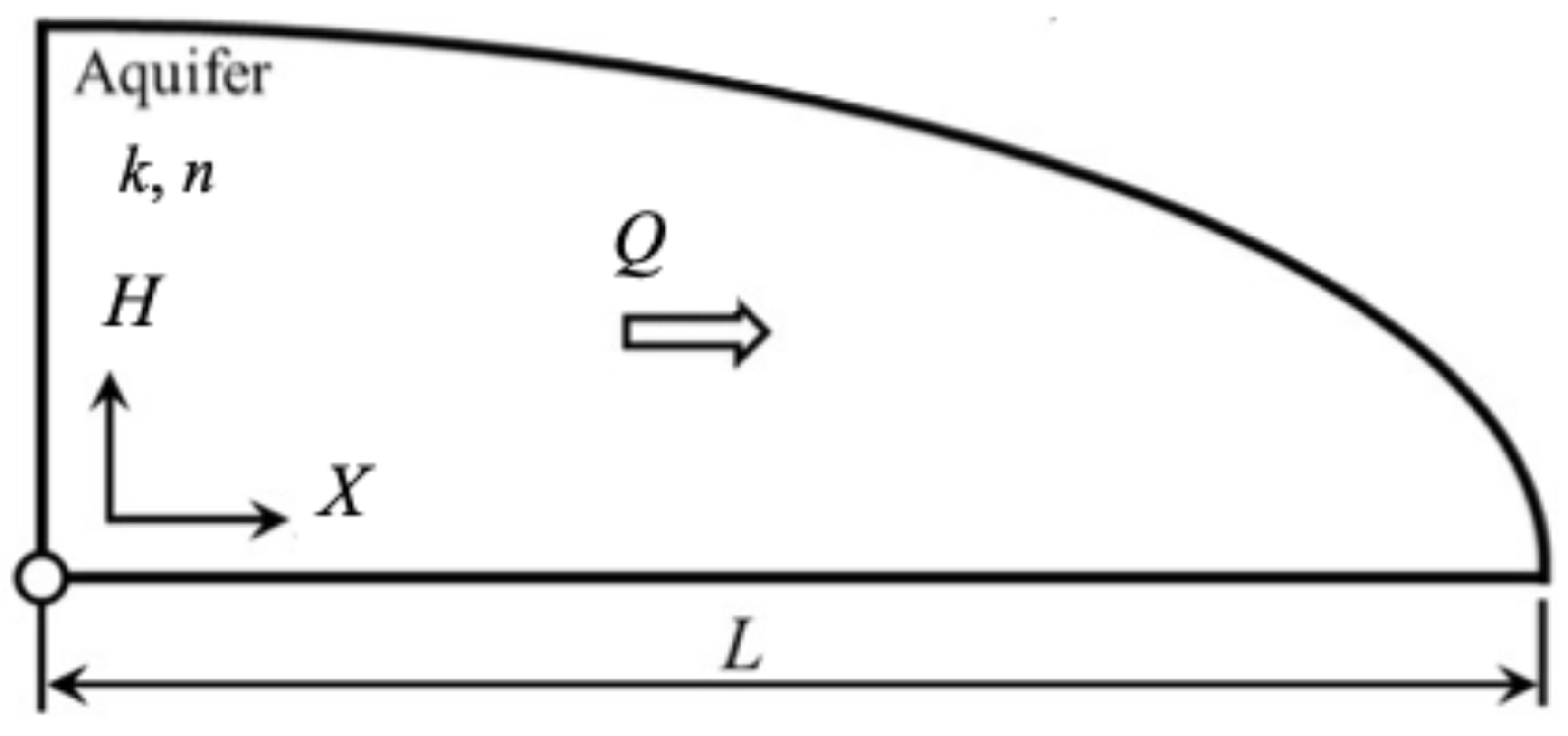
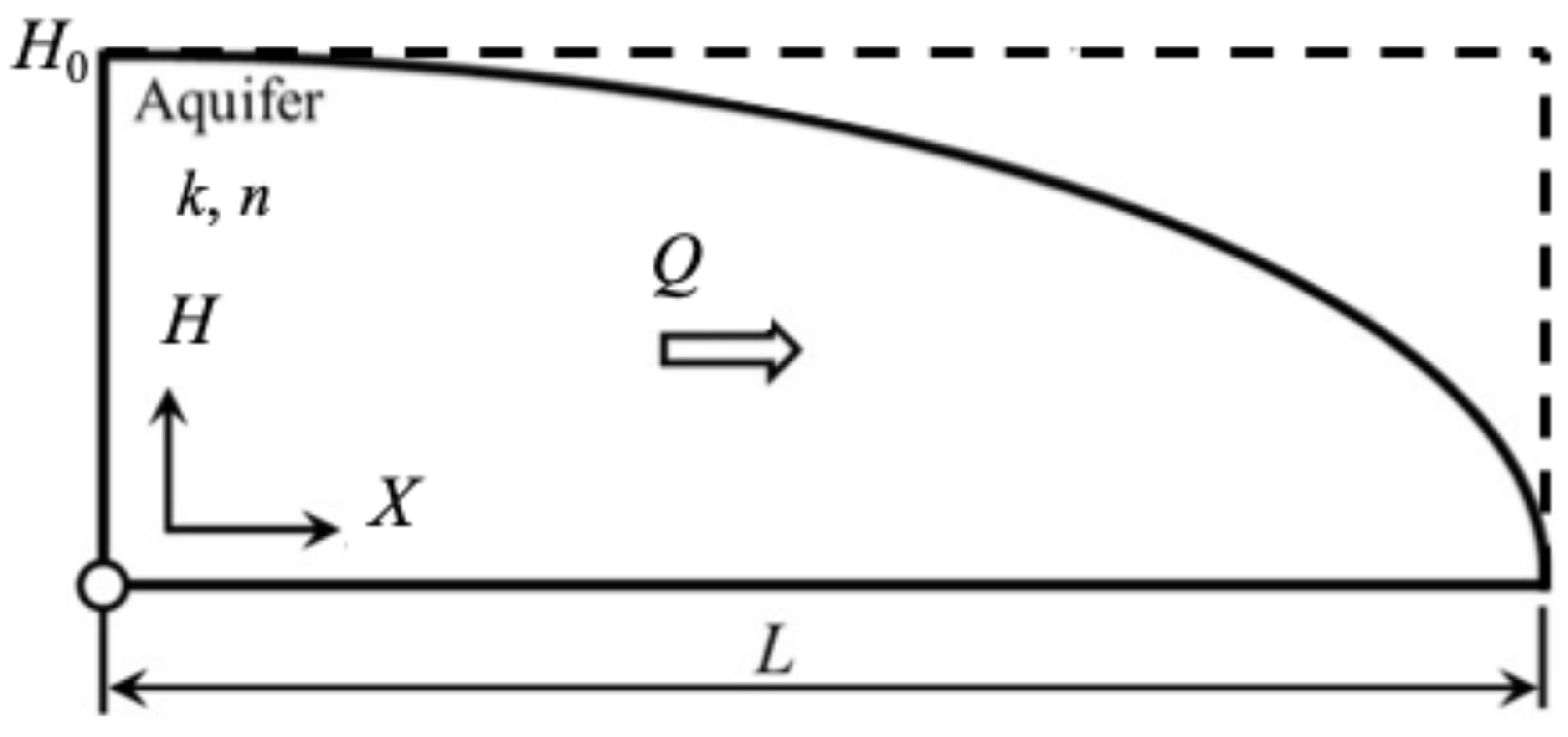
The formulation to be presented incorporates common assumptions in aquifer modeling, particularly addressing the drainage phase of a horizontal aquifer following the recharge period. The aquifer is assumed to be horizontal with a flat bed and uniform hydraulic properties both spatially and temporally. We will assume uniform and constant hydraulic conductivity (k) and drainable porosity (n) throughout the aquifer, with the resulting flow considered saturated and effectively one-dimensional. The impermeable bottom of the aquifer is also assumed to be flat and horizontal. A diagram of the aquifer with its main characteristics is provided in Figure 1.

This work’s findings can be applied to certain types of reservoirs, such as alluvial aquifers, which are primarily composed of unconsolidated sediments of various grain sizes, including gravel, sand, silt, and clay, deposited by rivers and streams. These aquifers often exhibit relatively homogeneous properties and flat horizontal beds over large areas, making them suitable for one-dimensional approximations. Another applicable reservoir type is found in deltaic environments, where sediments are deposited in deltas and can form flat horizontal beds, especially in regions further from the deltaic front. Coastal aquifers, which consist of sedimentary deposits laid down under uniform depositional conditions, also meet the assumptions necessary for applying the Boussinesq Equation. This section aims to summarize established results to ensure our presentation is comprehensive.

Dupuit–Forchheimer approximation, links the flow per unit of width for each time instant, T, and for each position, X, over the application area (0 < X < L), with the hydraulic parameters and the water profile depth [3,4,5] through

Q = - k H \frac{\partial H}{\partial X}

(1)

where H(X,T) is the water table’s depth at position X and at time T and k is the hydraulic conductivity. The continuity Equation (describing the mass conservation) expresses that the total amount of water flowing in any part of the aquifer locally (zero in the case of pure drainage) equals the sum of the amount of water flowing through it, ∂Q/∂X, plus the change in the storage capacity, n ∂H/∂T, which in the case of pure drainage without any recharging, is written as follows:

n \frac{\partial H}{\partial T} + \frac{\partial Q}{\partial X} = 0

(2)

where n is the drainable porosity. Combining Equations (1) and (2), we obtain the Boussinesq Equations (1)–(3) for the horizontal aquifer during pure drainage as follows

n \frac{\partial H (X, T)}{\partial T} = \frac{k}{2} \frac{\partial^{2} H^{2} (H, T)}{\partial X^{2}}

(3)

where, k (m s⁻¹) is the hydraulic conductivity, H (m) is the water profile depth as a function of time, T (s), and of the horizontal dimension 0 < X (m) < L, over the whole application area. The previous non-linear differential Equation may be subjected to various boundary conditions depending on the nature of the problem, with the most common approximations the imposing of a zero depth at the outer bound,

H (L, T) = 0

(4)

and a zero-flow, Q = 0, condition at the beginning implying a locally horizontal profile,

H' (0, T) = 0

Q (0, T) = {\frac{\partial H}{\partial X}|}_{X = 0} = 0

(5)

These boundary conditions (4 and 5) will be used in the analysis that follows. Integrating Equation (3) (local conservation of mass) along the entire aquifer and considering the zero-inflow boundary condition (4) we find that

\frac{d \tilde{S} (T)}{d T} + Q_{o u t} (T) = 0

(6)

where the total water storage

\tilde{S} (T)

\tilde{S} (T) = n \int_{0}^{L} H (X, T) d X

(7)

and the outflow is

Q_{o u t} (T) = Q (L, T) = - \frac{k}{2} {\frac{\partial H^{2} (H, T)}{\partial X}|}_{X = 1}

(8)

The total mass conservation (6) is a useful guide both in the construction of approximate solutions and models [23,24,25] as well as in phenomenological analyses with realistic applications in hydrology, e.g., as in [25]. It will serve as an important tool in our present work. In order to complete with the description of the problem in hand, an initial condition must be specified. The most interesting and clearly well separated initial conditions found in the literature for the pure drainage case, is either the steady state after infinite constant recharge analyzed in detail in [23,24]

H (X, 0) = H_{0} \sqrt{1 - \frac{X^{2}}{L^{2}}}

(9)

or a uniform initial water depth [7,26,27,28,29,30], i.e.,

H (X, 0) = H_{0}

(10)

In the following sections we will present a novel method for approximating the solution of Equation (3) using the boundary conditions (4,5) with initial conditions as (9) and (10), which are presented in Figure 2. The applicability of our solution to reasonable initial conditions between these two ones will be also discussed.

2.1. Dimensionless Form of the Boussinesq Equation during Pure Drainage

The dimensional hydraulic and geometrical parameters employed in the Boussinesq Equation (3) set-up are the horizontal aquifer’s length, L (m), the hydraulic conductivity, k (m s⁻¹), and the initial depth at X = 0, H₀ = H(0,0) (m). In a sense, the latter can be interpreted as a reminiscence of the recharging phase that led to each specific initial condition of the pure drainage to be studied. Making use of these basic scales we may rewrite Boussinesq Equation (3) during pure drainage in its dimensionless form

h (x, t) = \frac{1}{2} \frac{\partial^{2} h^{2} (x, t)}{\partial x^{2}}

(11)

where the main dimensional parameters H, X, T have been replaced by their dimensionless analogs

h = \frac{H}{H_{0}}, x = \frac{X}{L}, t = \frac{k H_{0} T}{n L^{2}}

(12)

In this dimensionless form the flow rate becomes

q = \frac{Q L}{k H_{0}^{2}} = - h \frac{\partial h}{\partial x}

(13)

The boundary conditions in the dimensionlees form read

h (1, t) = 0, q (0, t) = {\frac{\partial h}{\partial x}|}_{x = 0} = 0

(14)

and the initial conditions (9) and (10) that will be mainly studied become

h (x, 0) = \sqrt{1 - x^{2}}

(15)

for an initially steady state flow after recharging of infinite time, and

h (x, 0) = 1

(16)

for an initially uniform horizontal water table. Integrating Equation (11) along the entire aquifer and utilizing the zero-inflow boundary condition (14) we conclude with the dimenssionless form of the water balance Equation (6), that is

\frac{d S (t)}{d t} + q_{o} (t) = 0

(17)

where the dimensionless storage

S (t)

S (t) = \int_{0}^{1} h (x, t) d x

(18)

and the dimensionless outflow is

q_{o} (t) = q (1, t) = - \frac{1}{2} {\frac{\partial h^{2} (x, t)}{\partial x}|}_{x = 1}

(19)

2.2. Series Expansion and Late-Time Asymptotic Analysis of the Water Table during Pure Drainage

For the case of groundwater flowing in a horizontal finite aquifer at a zero-recharge rate, the solution of the Bussinesq Equation can be obtained by assuming the separation of variables [2,3,7]. This is actually an exact asymptotic solution of the horizontal aquifer recession phase for late times. Following a slightly modified, for the needs of the work that will follow, but equivalent analysis with Bussinesq [1,2], we will write the water profile in the form

h (x, t) = h_{o} (t) s (x, t)

(20)

where

h_{o} (t)

is the water depth at x = 0,

h_{o} (t) = h (0, t)

(21)

which reflects the evolution of the relative depth of the water table, which normally decreases during the pure drainage phase. On the other hand,

s (x, t)

incorporates any change in the shape of the water table during the drainage phase. Noting that

h (x, t)

and, correspondingly,

s (x, t)

and

s^{2} (x, t)

are even functions of x, we proceed with series expansion of

s (x, t)

as follows.

s^{2} (x, t) = 1 - a_{1} (t) x^{2} + a_{2} (t) x^{4} + a_{3} (t) x^{6} + \dots

(22)

where, in order to satisfy all the proper boundary conditions,

s (0, t) = 1, s (1, t) = 0, {\frac{\partial s}{\partial x}|}_{x = 0} = 0

(23)

the sum of the parameters

a_{i} (t)

, should equal

a_{1} (t) = 1 + \sum_{i = 2}^{\infty} a_{i} (t)

(24)

After substituting of

h (x, t)

given by Equation (20) in the Boussinesq Equation (11), we derive its equivalent form

{\dot{h}}_{o} (t) s (x, t) + h_{o} (t) \dot{s} (x, t) = \frac{h_{0}^{2} (t)}{2} \frac{\partial^{2} s^{2} (x, t)}{\partial x^{2}}

(25)

The reader should have noticed that in the previous Equations (25) we have used dot notation to refer to the time derivative d/dt, to facilitate the writing of the rather long Equations. This notation will be used for the rest of the work.

Taking the limit of Boussinesq Equation (25) at x = 0, and noting that

s (0, t) = 1

from (23), we conclude that the evolution of

h_{o} (t)

depends solely on

a_{1} (t)

through

\frac{\dot{h_{o}} (t)}{h_{o}^{2} (t)} = - \frac{d {h_{o}}^{- 1} (t)}{d t} = \frac{1}{2} {\frac{\partial^{2} s^{2} (x, t)}{\partial x^{2}}|}_{x = 0} = - a_{1} (t)

(26)

Calculating higher derivatives of even order, in terms of x, of Boussinesq Equation (25) and taking its limit at x = 0, we see that the evolution of the parameters

a_{i} (t)

, in ascending order, is also linked to the evolution of

a_{1} (t)

. For instance, by calculating the second derivative versus x of Equation (25), and taking the limit at x = 0 we derive

a_{2} (t)

as a function of

a_{1} (t)

{{12 a}_{2} (t) = {a_{1}}^{2} (t) - h}_{o}^{- 1} (t) {\dot{a}}_{1} (t)

(27)

By calculating the

f o r t h d e r i v a t i v e

we derive

a_{3} (t)

, as a function of

a_{1} (t)

and

a_{2} (t)

360 a_{3} (t) = 2 a_{1}^{3} (t) - 5 a_{1} (t) {\dot{a}}_{1} (t) h_{o}^{- 1} (t) + 12 {\dot{a}}_{2} (t) h_{o}^{- 1} (t)

(28)

and so on. In its general form, the evolution of the

a_{i} (t)

for i >1, is calculated through the following limit

\frac{1}{h_{o}^{2} (t)} \frac{d}{d t} (h_{o} (t) {\frac{\partial^{2 i - 2} s (x, t)}{\partial x^{2 i - 2}}|}_{x = 0}) = \frac{1}{2} {\frac{\partial^{2 i} s^{2} (x, t)}{\partial x^{2 i}}|}_{x = 0} = \frac{(2 i)!}{2} a_{i} (t)

(29)

This analysis reveals the central role of

a_{1} (t)

in controlling the evolution of the water table,

h (x, t) = h_{o} (t) s (x, t)

. In other words, knowing the exact behavior of

a_{1} (t)

means that we may determine the evolution of the shape in a desired accuracy, depending on the terms we keep in the series expansion of

s (x, t)

as it will be discussed and applied in the next section.

When all the time derivatives in the shape formation vanish (i.e., in Equations (27) and (28)), all

a_{i} (t)

reach their finite values resulting into a late time shape

s (x)

independent of time, which is a function of x only. All parameters are taken finite values that depend solely on the finite value,

α_{1 f},

of the controlling parameter

α_{1}

, and the shape function becomes

s (x) = \sqrt{1 - α_{1 f} x^{2} + \frac{{α_{1 f}}^{2}}{12} x^{4} + \frac{{α_{1 f}}^{3}}{180} x^{6} + \frac{{α_{1 f}}^{4}}{720} x^{8} + \frac{{α_{1 f}}^{5}}{2025} x^{10} \dots}

(30)

where we present terms up to the 5th order.

Unfortunately, Equation (30) cannot be written as an explicit infinite sum. Each term of order i should be calculated separately, using respectively the (2i-2)-order derivative versus x of Bousinesq Equation (25), through Equation (29), and all previous terms of lower order. Still, Equation (30) together with Equation (26) and the presented analysis offer an interesting interpretation focusing on the main mechanisms of profile deformation and may serve as a nice and effective modelling tool as it will be shown in the later.

The late time behavior of the water table and its constant shape can be explicitly described by the analysis given in [2,7] by applying separation of variables in Boussinesq Equation. Equivalently, in the direction of our interpretation so far, when the profile reaches a constant shape

s (x),

Boussinesq Equation (25) simplifies to

{\dot{h}}_{o} (t) s (x) = \frac{h_{0}^{2} (t)}{2} \frac{\partial^{2} s^{2} (x)}{\partial x^{2}}

(31)

where the separation of the variables is now clear and physically well justified. Recalling the result of Equation (26),

\frac{\dot{h_{o}} (t)}{h_{o}^{2} (t)} = - a_{1} (t)

, we realize that Equation (31) should satisfy

\frac{\dot{h_{o}} (t)}{h_{o}^{2} (t)} = \frac{1}{2} \frac{\partial^{2} s^{2} (x)}{\partial x^{2}} = c = - a_{1 f}

(32)

where

a_{1 f}

must be greater than zero,

a_{1 f} >

0. Equation (21) can be fed an arbitrary initial condition

h_{o} (0) = h_{0}

(33)

and boundary conditions as in Equation (23),

s (1) = 0, s (0) = 1, {s' (x)|}_{x = 0} = 0

(34)

The general solution of (32) for the profile, satisfying the first and the third of the boundary conditions (34), is expressed in the form of the inverse function

x = 1 - s^{2} (x) \frac{{\sqrt{3}}_{2} F_{1} (\frac{1}{2}, \frac{2}{3}, \frac{5}{3}, s^{3} (x))}{2 \sqrt{2 α_{1 f}}}

(35)

where ₂F₁ is the ordinary hypergeometric function. Furthermore, using the boundary condition at x = 0,

s (0) = 1

allows the calculation of the finite value of

α_{1}

, that equals

α_{1 f} = \frac{{\sqrt{3}}_{2} F_{1} (\frac{1}{2}, \frac{2}{3}, \frac{5}{3}, 1)}{\sqrt{8}} = \frac{3 π}{8} \frac{{Γ (\frac{5}{3})}^{2}}{{Γ (\frac{7}{6})}^{2}} \approx 1.11552

(36)

After that, the finite shape storage factor (i.e., the storage of the finite shape of the water table)

S_{o f} = S / h_{o} = \int_{0}^{1} s (x) d x = \int_{0}^{1} x d s

, can be calculated as

S_{ο f} = \frac{4 Γ (\frac{7}{6})}{3 \sqrt{π} Γ (\frac{5}{3})} \approx 0.773064

(37)

On the other direction, the solution of Equation (32) for the time dependent part,

h_{ο} (t)

, becomes

h_{ο} (t) = \frac{1}{h_{0}^{- 1} + a_{1 f} t}

(38)

and correspondingly the storage at late times evolves as

S (t) = S_{o} h_{ο} (t) = \frac{S_{o f}}{h_{0}^{- 1} + a_{1 f} t}

(39)

and the outflow,

q_{o} (t),

associated with the late time analysis reads

q_{o} (t) = - \dot{S} (t) = \frac{a_{1} S_{o f}}{{{(h}_{0}^{- 1} + a_{1 f} t)}^{2}}

(40)

Of course, the slope of the squared profile at the outer bound, x = 1, satisfies the mass conservation,

\frac{1}{2} {\frac{\partial h^{2} (x, t)}{\partial x}|}_{x = 1} = \frac{h_{o}^{2} (t)}{2} {\frac{d s^{2} (x)}{d x}|}_{x = 1} {= - q}_{o} (t)

(41)

concluding that the slope of the squared shape function,

s^{2} (x),

at x = 1 is

- \frac{1}{2} {\frac{d s^{2} (x)}{d x}|}_{x = 1} = a_{1 f} S_{o f} \approx 0.86237

(42)

The above analysis and the findings regarding the central role of

a_{1}

in the water profile formation and the late time asymptotic character of the solution will serve as the basis for constructing in the following an accurate model, that mimics the exact Boussinesq Equation in reproducing many features of the evolution of the water table during drainage.

3. A New Model for the Drainage Phase of Horizontal Unconfined Aquifer

Capitalizing on the previous Section 2.3, we constract in the following a model for the accurate derivation of the evolution of parameter

a_{1} (t)

. As we explained in detail, having

a_{1} (t)

means determining the evolution of both the water table head

h_{o} (t)

and the shape of the profile

s (x, t)

, in an accuracy that depends on how many terms

a_{i} (t)

are used. To our knowledge there is no other work emphasizing on the evolution of

a_{1} (t)

making our findings quite novel. The model offers new insight in describing and understanding the water table modifications during drainage and can serve as an efficient modelling tool.

In the direction of the previous analysis, we use the expansion presented in Equations (20)–(22) expressing the water profile as

h (x, t) = h_{o} (t) s (x, t)

(43)

keeping as many terms as we need, up to the desired order

x^{2 ν}

, thus approximating

s (x, t)

s^{2} (x, t) = 1 - a_{1} (t) x^{2} + \sum_{i = 2}^{ν - 1} a_{i} (t) x^{2 i} + (a_{1} - 1 - \sum_{i = 2}^{ν - 1} a_{i} (t)) x^{2 ν}

(44)

to conform all boundary conditions (23). To satisfy mass conservation, we introduce (43) into the mass balance Equation (17),

\frac{d S}{d t} = \frac{1}{2} {\frac{d h^{2} (x, t)}{d x}|}_{x = 1}

, deriving

\frac{d h_{o} (t) S_{o} (a_{1}, a_{2}, \dots)}{d t} = {\frac{1}{2} h}_{o}^{2} (t) {\frac{\partial s^{2} (x, t)}{\partial x}|}_{x = 1}

(45)

where

S_{o} (t)

, is the shape storage factor

S_{o} (t) = \int_{0}^{1} s (x, t) d x

(46)

and is a function of the model’s parameters

a_{i} (t)

. Noting also, that the slope of the squared shape function

s^{2} (x, t)

by Equation (44) at x = 1 is

{\frac{\partial s^{2} (x, t)}{2 \partial x}|}_{x = 1} = - ν + (ν - 1) a_{1} - \sum_{i = 2}^{ν - 1} (ν - i) a_{i}

(47)

and using the result of Equation (26)

\frac{\partial h_{o}^{- 1} (t)}{\partial t} = a_{1} (t)

(48)

the mass conservation Equation (45) yields

a_{1} S_{o} - h_{o}^{- 1} \sum_{i = 1}^{ν - 1} \frac{\partial S_{o}}{\partial a_{i}} {\dot{a}}_{i} = ν - (ν - 1) a_{1} + \sum_{i = 2}^{ν - 1} (ν - i) a_{i}

(49)

which is the core of the present model’s formulation. Note that although in (49) we omitted writing explicitly the time dependence, the reader should still consider that all parameters are functions of time,

a_{i} = a_{i} (t) .

The Equation (49) forms a close system together with the relations for the evolution of

a_{i} (t)

coming out by the (2i-2)-order derivative versus x of Boussinesq Equation (25) through Equation (29), as analyzed in the previous section. This system constitutes the main modelling idea of this work and will be used extensivelly in the following.

At late times, when all time derivatives of

a_{i}

vanish in the model’s Equation (49)

a_{1}

reaches a finite state

a_{1 f}

, and successively through Equation (29) all the rest of the parameters

a_{i}

are taken finte values depending on

a_{1 f}

a_{2 f} = \frac{{α_{1 f}}^{2}}{12}, a_{3 f} = \frac{{α_{1 f}}^{3}}{180}, a_{4 f} = \frac{{α_{1 f}}^{4}}{720}, a_{5 f} = \frac{{α_{1 f}}^{5}}{2025} \dots

(50)

Thus, the profile takes a constant shape, depends solely on

a_{1 f}

. The finite value of

a_{1}

, becomes then a function of the order ν of the model Equation (49). In other words, it depends on the number of the terms that are used in the expansion (44), by solving the steady form of the mass balance Equation (49) which is expressed through

a_{1 f} S_{o f} = ν - (ν - 1) a_{1 f} + \sum_{i = 2}^{ν - 1} (ν - i) a_{i f}

(51)

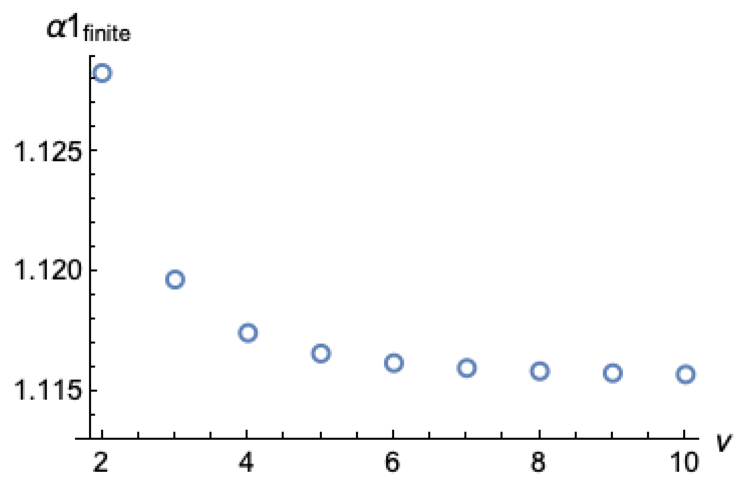
where, any time dependence has been removed. The gradual approach of

a_{1 f}

to its exact value given by eq. (36) as the order ν of the model (49) increases, is shown in Figure 3.

3.1. Analysis and Application of the New Model

Seeking for the best combination between accuracy and lack of complexity, we present a full analysis approximating the expansion (44) to the 6th order of x. In fact, the same analysis can be undertaken using an approximation of the 8th order (the upper end of the meaningful model’s choices, in our opinion) in a similar manner, but the difficulty which is added while improving accuracy obscures the clarity of the presentation.

Specifically, by setting ν = 3, in Equation (44), we select a 6th in terms of x, expansion of the profile shape of the form

s (x, t) = \sqrt{1 - a_{1} x^{2} + a_{2} x^{4} + {(a_{1} - 1 - a}_{2}) x^{6}}

(52)

Correspondingly, Equation (48) for the evolution of

a_{1} (t)

becomes

a_{1} S_{o} (a_{1}, a_{2}) - \frac{(S_{o, α_{1}} {\dot{a}}_{1} + S_{o, α_{2}} {\dot{a}}_{2})}{h_{o}} = (3 - 2 a_{1} + a_{2})

(53)

In Equation (53), the storage

S_{o} (a_{1}, a_{2})

must be calculated numerically through the integral

S_{o} (t) = \int_{0}^{1} \sqrt{1 - a_{1} x^{2} + a_{2} x^{4} + {(a_{1} - 1 - a}_{2}) x^{6}} d x

(54)

while the partial derivatives

S_{o, α_{1}}

and

S_{o, α_{2}}

are calculated respectively through

S_{o, α_{1}} = \frac{\partial S_{o}}{\partial a_{1}} = \frac{1}{2} \int_{0}^{1} \frac{- x^{2} + x^{6}}{\sqrt{1 - a_{1} x^{2} + a_{2} x^{4} + (a_{1} - 1 - a_{2}) x^{6}}} d x

(55)

and

S_{o, α_{2}} = \frac{\partial S_{o}}{\partial a_{2}} = \frac{1}{2} \int_{0}^{1} \frac{x^{4} - x^{6}}{\sqrt{1 - a_{1} x^{2} + a_{2} x^{4} + (a_{1} - 1 - a_{2}) x^{6}}} d x

(56)

Equation (53) forms a close system, in the context we presented, together with Equations (48) for

{\dot{h_{o}^{- 1}} = a}_{1}

, and (27) for

a_{2} = (a_{1}^{2} - h_{o}^{- 1} {\dot{a}}_{1}) / 12

Before proceeding with the numerical solution of the defined system of Equations, we will give a closer look at the late time behavior of this model. As the time derivatives vanish, the specific system of Equations drives

a_{1}

to a finite value (Figure 3), which can be found by solving Equation (49). With our setting ν = 3, this corresponds to solving

a_{1} S_{o} = 3 - 2 a_{1} + \frac{a_{1}^{2}}{12}

(57)

resulting to

a_{1 f} = 1.11966

. Then,

a_{2 f} = \frac{{1.11966}^{2}}{12} =

0.10447 and the finite shape function s(x) corresponds to a finite storage factor which is calculated (numerically) through (54) equal to

S_{o f} = 0.77269 .

Thus, the slope of the squared shape function (42) becomes

a_{1 f} S_{o f} = 0.86515

. These results are close but surely not identical to the exact asymptotic values given in Equations (35), (36) and (41) from the exact solution of the Boussinesq Equation.

We may refine the above values by slightly modifying the exact Equation (27) introducing a parameter

c_{1}

{12 a}_{2} = (c_{1} a_{1}^{2} - h_{o}^{- 1} {\dot{a}}_{1})

(58)

This modification drives

a_{2}

to a finite value of

a_{2 f} = c_{1} \frac{a_{1 f}^{2}}{12}

(59)

Although affecting the exact character of Equation (27), we should keep in mind that the whole procedure we describe is an approximate solution, which we try making as accurate as possible. Using (58) instead of (27) gives the advantage of tuning the finite behavior of the solution towards more accurate values. Furthermore, this modification does not affect seriously the observed accuracy of the model at early times, where other type of problems should be handled as it will be shown.

By using

c_{1}

as tuning parameter, we may seek the choice resulting to the most accurate finite state through Equation (57) which now reads

a_{1 f} S_{o} = 3 - 2 a_{1 f} + c_{1} \frac{a_{1 f}^{2}}{12}

(60)

More specifically we seek the value of

c_{1}

producing as accurate as possible finite values for

a_{1 f}

S_{o f}

, as well as for the slope of the squared profile. We have concluded that the best choice is

c_{1} = 0.9 .

Using this value, we calculate,

a_{1 f} = 1.1156,

S_{o f} = 0.7731

and the slope of the squared shape

a_{1 f} S_{o f} = 0.8622

showing agreement up to the 4th decimal, when compared to the respective exact results of the Boussinesq Equation.

At this point, we must note that in the case of an 8th order expansion model (ν = 4) the added degree of freedom will guarantee exact match of all three previous profile features,

a_{1 f}

S_{o f}

, and correspondingly

a_{1 f} S_{o f},

by modifying properly the extra Equation (28) for

a_{3}

, to close the model, with the inclusion of another one tuning parameter

c_{2}

through

360 a_{3} = 2 c_{2} a_{1}^{3} - 5 a_{1} {\dot{a}}_{1} (t) h_{o}^{- 1} + 12 {\dot{a}}_{2} h_{o}^{- 1} (t)

(61)

In that case the finite value of

a_{3 f}

is,

a_{3 f} = c_{2} \frac{a_{1}^{3}}{180}

, and the finite value for

a_{1 f}

comes through solving the analog of Equation (60) for the next higher order,

a_{1 f} S_{o} = 4 - 3 a_{1 f} + 2 c_{1} \frac{a_{1 f}^{2}}{12} + c_{2} \frac{a_{1 f}^{3}}{180}

(62)

finding the pair of (

c_{1}

c_{2}

) corresponding to the exact Boussinesq values for

a_{1 f}

and

S_{o f}

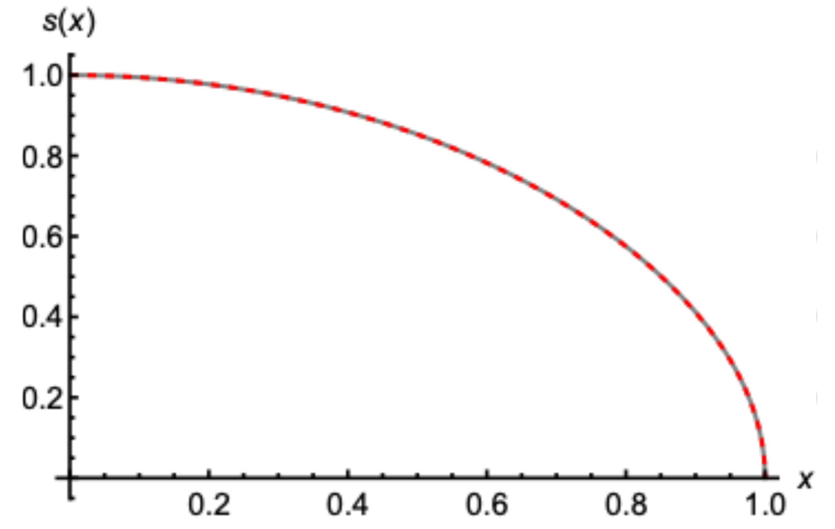
In Figure 4, we present the finite profile shape of the introduced 6th order model

s (x) = \sqrt{1 - 1.1156 x^{2} + 0.1037 x^{4} + 0.019 x^{6}}

(63)

and the late time exact Boussinesq solution by Equation (35). The coincidence between the two profiles is remarkable. In fact, their difference, at its most, does not exceed 1%₀. Also, in Figure 5, Figure 6 and Figure 7 we present the numerical solution of the full system of the model’s Equations (53,48,58) for the evolution of the profile during drainage, where three different initializations were used to test the model’s efficiency.

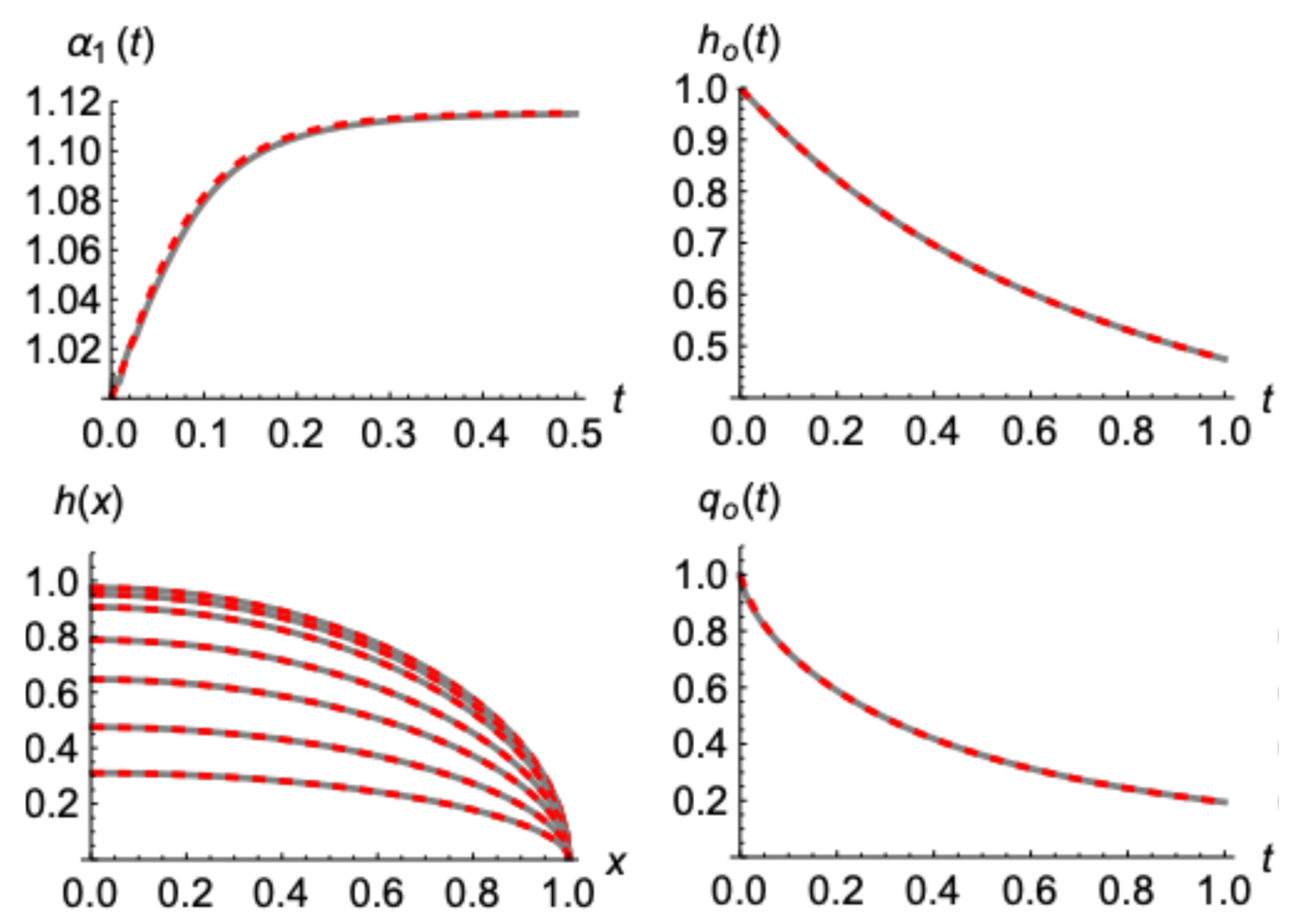
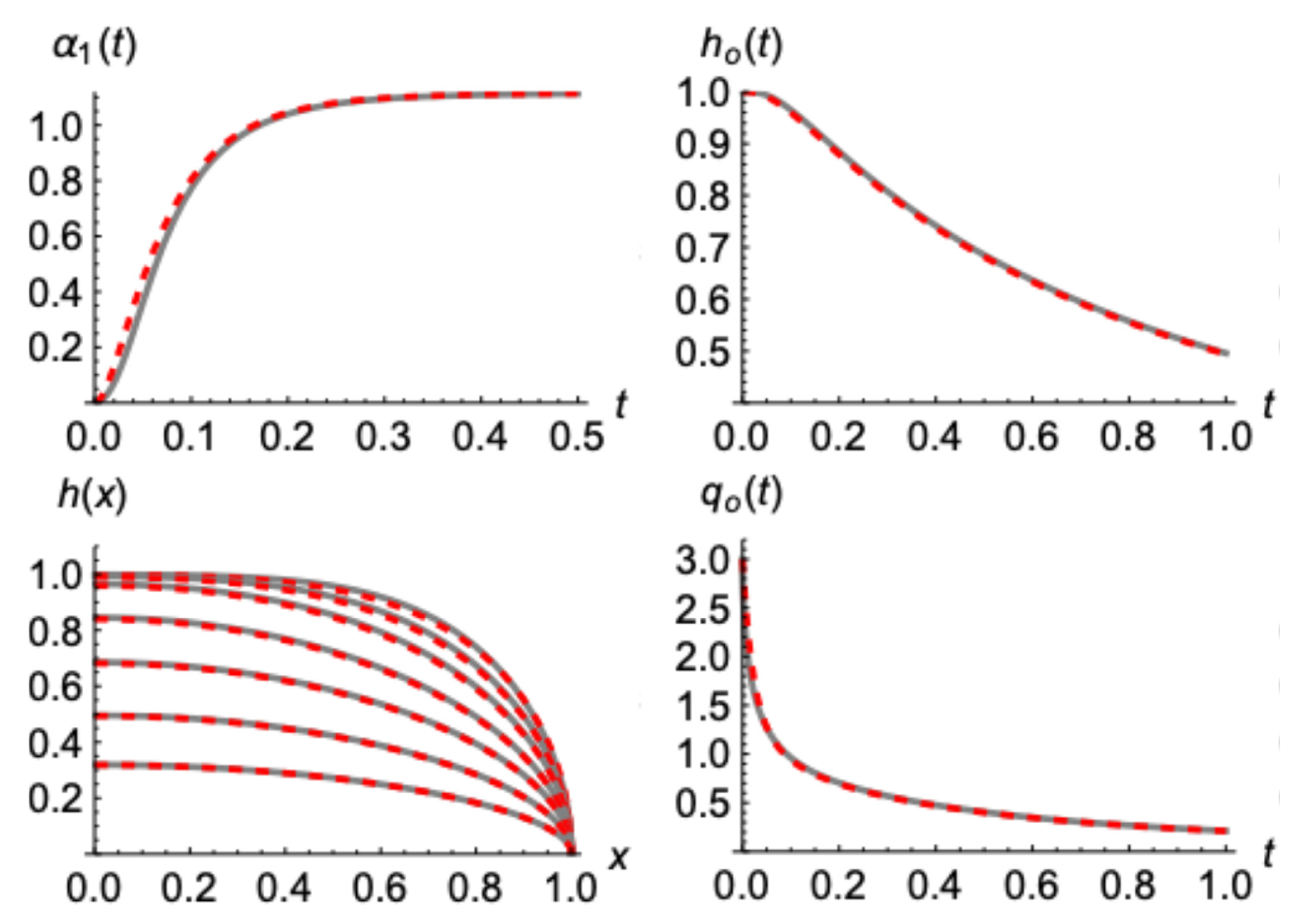
Specifically, in Figure 5 the case starts with steady state after uniform recharging; thus, the initial profile is

h (x, 0) = \sqrt{1 - x^{2}}

. The presented results refer to the evolutions of parameter

a_{1} (t)

, water table head,

h_{o} (t) = h (0, t)

, water table

h (x, t)

and outflow

q_{o} (t)

. As it is shown, the resemblance of the model’s solution to the exact numerical solution of the Boussinesq Equation (11) is quite impressive. Even regarding the outflow, the most difficult parameter to capture accurately, since it is affected by the whole water profile’s development, the coincidence is very good. Besides a relative difference at very early times that will be discussed next, the model performs very accurately.

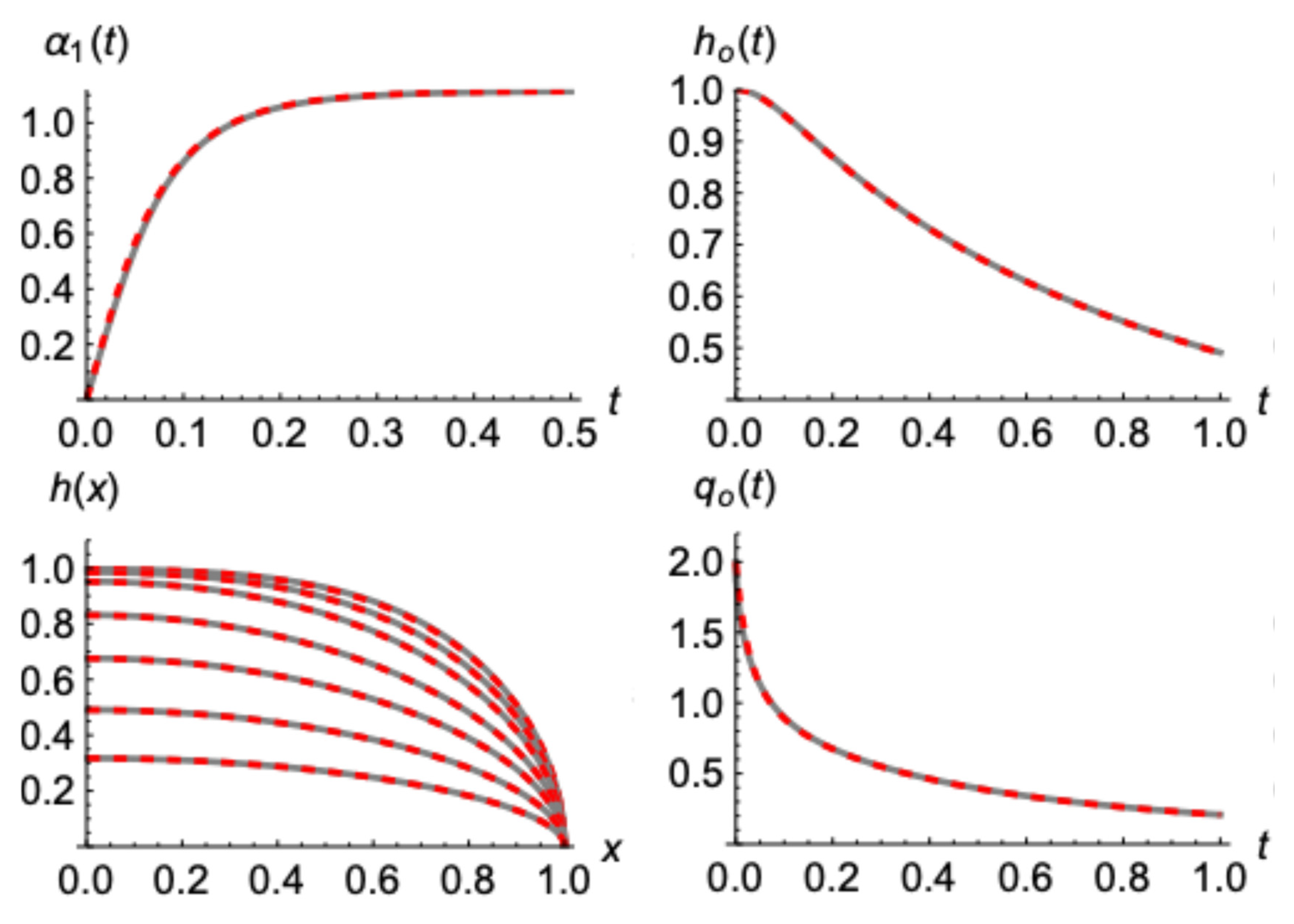
In Figure 6 and Figure 7, similar results are presented, for initial water tables of the forms

h (x, 0) = \sqrt{1 - x^{4}}

and

h (x, 0) = \sqrt{1 - x^{6}}

respectively. The comparison remains adequately good and in favor of the presented model (49).

Taking a closer look, however, at the behavior of the outflow at very early times (Figure 8), we realize that there is some discrepancy which increases as the initial outflow (thus the slope of the shape of the squared profile) becomes bigger.

This deviation can be attributed to the fact that the presented sharp initial water tables aiming to emulate the end of a recharging period, impose different physical

characteristics compared to drainage profiles since they are not a solution of the same Equation. Specifically, Boussinesq Equation (11) during pure drainage, with a zero-water depth (constant in the more general case) at the end of the aquifer, at x = 1, implies that the second derivative of the squared water profile versus x vanishes. This is not the case during recharge periods as well as in none of the previously presented examples. To conform then the imposed initial profile, Boussinesq concludes with a “violent” modification, resulting into a sudden change of outflow at an infinite rate as it will be shown. Multiplying Boussinesq Equation (11), during drainage, by h(x,t) and differentiating versus x, yields

\frac{\partial}{\partial x} (\frac{1}{2} \dot{h} (x, t)) = \frac{\partial}{\partial x} h (x, t) \frac{1}{2} \frac{\partial^{2} h^{2} (x, t)}{\partial x^{2}} + h (x, t) \frac{1}{2} \frac{\partial^{3} h^{2} (x, t)}{\partial x^{3}}

(64)

Taking the limit of Equation (64) at x = 1 and substituting

q_{o} (t)

by Equation (19), we see that the time derivative of the outflow

{\dot{q}}_{o} (t)

equals

{\dot{q}}_{o} (t) = - {\frac{\partial h (x, t)}{\partial x}|}_{x = 1} {\frac{1}{2} \frac{\partial^{2} h^{2} (x, t)}{\partial x^{2}}|}_{x = 1}

(65)

From Equation (65) becomes evident that, since the slope of the water profile at x = 1 is infinite, in order of

{\dot{q}}_{o} (t)

to be definite the second derivative of the squared profile must be zero. Otherwise

{\dot{q}}_{o} (t)

is also infinite. Such a behavior is, strictly speaking, over the capabilities of the presented model, and demands different approximations to evolve up to a point that the model can accurately handle. Such a case is presented in Figure 9, for an initial squared profile with zero second derivative at x=1, slightly different than the one presented in Figure 5. In this case the coincidence between the present model and the Boussinesq solution is almost perfect.

Modeling the very early time drainage and matching with the present model later on, is the subject of the following section.

3.2. The Case of a Sudden Drawdown from an Initially Horizontal Water Table

This is a case well studied in literature [7,26,27,28,29,30] resempling at the early stages the semi-infinite aquifer [26,27]. In a sense, it is an extreme example for applying modelling ideas starting with an infinitelly sharp step—change. Still it offers a great basis for analytic description and approximate solutions [36,37,38]. Our presented approximated solution cannot handle accurately directly such extreme profiles, as it was discussed earlier. However, intermediate modelling ideas can be used to confront such rough changes till the profile reaches a more smooth shape that can be fed to the newlly proposed model.

3.2.1. Early Time Approximation

We approximate the early behavior of the drainage through a “wave type” character, in a way relativelly similar to what [25] presented for the recharging built-up phase, of the form

h (x, t) = \{\begin{matrix} 1, x < 1 - Δ \\ Φ (\frac{x - 1 + Δ}{Δ}), 1 - Δ < x < 1 \end{matrix}

(66)

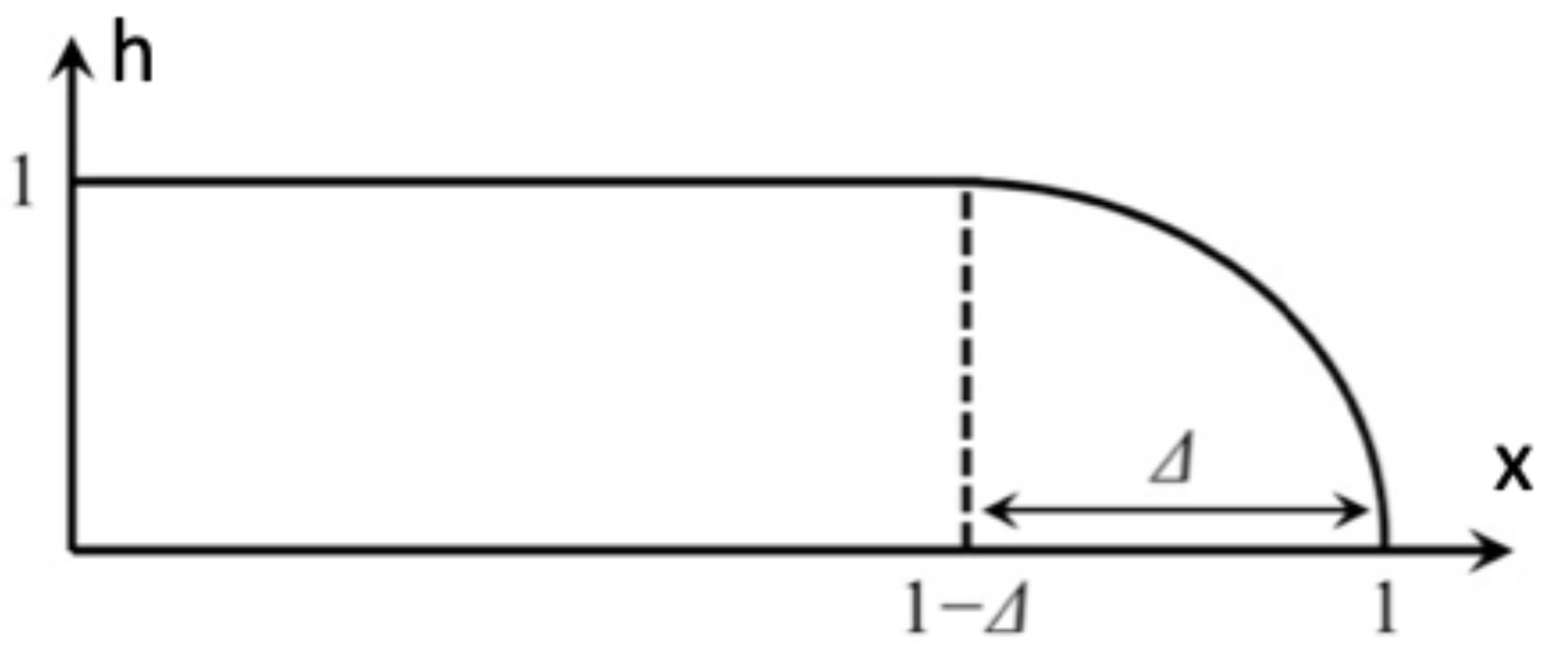
This means that the profile is uniform at the beginning and deforms gradually from the end point, x = 1, towards x = 0. The outflow affects the profile at a range Δ, starting from zero and increasing with time while keeping a constant shape

Φ (y)

in terms

y = \frac{x - 1 - Δ}{Δ}

resembling a wave in a sense, as shown in Figure 10.

The dimenssionless storage

S (t)

is calculated by integrating the profile given in (66) through

S (t) = \int_{0}^{1} h (x, t) d x = 1 - Δ (t) + Δ (t) \int_{0}^{1} Φ (y) d y

(67)

and by differentiation versus time, the outflow rate

q (t) = - \dot{S} (t)

reads

q (t) = - \dot{S} (t) = \dot{Δ} (t) (1 - \int_{0}^{1} Φ (y) d y)

(68)

Recalling the detailed analysis analysis given in [7,27] the actual outflow for this specific case of a sudden drawdown and drainage shows a behavior of the form

q (t) = s_{1} t^{- 1 / 2}

(69)

with

s_{1} \approx 0.33206

[7]. In order to reproduce this behavior by the modelled Equation (68), the velocity of the wave,

\dot{Δ} (t)

, must show a time dependence of the form

\dot{Δ} (t) = s_{1} {(1 - \int_{0}^{1} Φ (y) d y)}^{- 1} t^{- 1 / 2}

(70)

which, obviously, becomes infinite at the beginning of the drainage, in agreement with the initially infinite outflow rate at this specific case. Integrating Equation (70) over time results then into the model’s gradual displacement

Δ (t) = 2 s_{1} {(1 - \int_{0}^{1} Φ (y) d y)}^{- 1} t^{1 / 2}

(71)

What is remaining, is to specify a proper form for

Φ (y)

. In the same line with the analysis followed in the previous section, we assume that

Φ (y)

can be described by a polynomial of the form

Φ (y) = \sqrt{1 + a_{2} y^{4} + a_{3} y^{6} \dots + a_{ν} y^{2 ν}}

(72)

with

a_{ν} = - 1 - a_{2} - a_{3} - \dots - a_{ν - 1}

. The specific form satisfies the proper boundary conditions

Φ (0) = 1

and

Φ (1) = 0

and the absence of the

y^{2}

term guarantees the vanishing of the three first derivatives at y = 0, giving smooth transition between the two branches of the model (66). Furthermore, after the end of the functionality of the model (66), at the time when

Δ (t)

= 1 and the “wave” reaches the upper end at x = 0, the evolution of the water profile can be continued using the analysis presented at the previous section.

Making use of the mass-balance integrated Boussinesq Equation, the outflow should match the dimensionless slope of the squared profile at x = 1, through

q (t) = - \frac{1}{2} \lim_{x \to 1} \frac{\partial h^{2} (x, t)}{\partial x} = - {\frac{1}{2 Δ (t)} \frac{\partial Φ^{2} (y)}{\partial y}|}_{y = 1}

(73)

After calculating the dimensionless slope of the modeled

Φ^{2} (y)

at y=1

- \frac{Φ^{2}' (1)}{2} = ν + (ν - 2) a_{2} + (ν - 3) a_{3} \dots + 2 a_{ν - 2} + a_{ν - 1}

(74)

and introducing into Equation (73) the mass balance yields

{2 (1 - \int_{0}^{1} Φ (y) d y)}^{- 1} = \frac{ν + (ν - 2) a_{2} \dots + 2 a_{ν - 2} + a_{ν - 1}}{s_{1}^{2}}

(75)

which offers a closure of the “wave” model (66), linking the dimensionless storage

\int_{0}^{1} Φ (y) d y

with the parameters of the model,

a_{2}, a_{3} \dots

and so on. Actually, Equation (75) offers many degrees of freedom, thus, giving the opportumity to investigate and impose several specific features in the assumed “wave shape”. However, for the sake of simplicity and in the context of the previous section we will present the simplest meeningfull model with ν = 3, that is expressed as

Φ (y) = \sqrt{1 + a_{2} y^{4} + (- 1 - a_{2}) y^{6}}

(76)

By this choice, Equation (75) reduces to

{(1 - \int_{0}^{1} \sqrt{1 + {a_{2} y}^{4} - (1 + a_{2}) y^{6}} d y)}^{- 1} = \frac{3 + a_{2}}{2 s_{1}^{2}}

(77)

allowing for the direct numerical estimation of the proper value of

a_{2} = - 1.4818945

. With this value of

a_{2}

, the dimensionnless storage equals,

S_{o} = \int_{0}^{1} Φ (y) d y = 0.854735

. The model is valid up to the limiting time, t_max, when the “wave” reaches the upper end, at x = 0, which is calculated through Equation (71) and equals t_max = 0.0478442, for

Δ (t) = 1

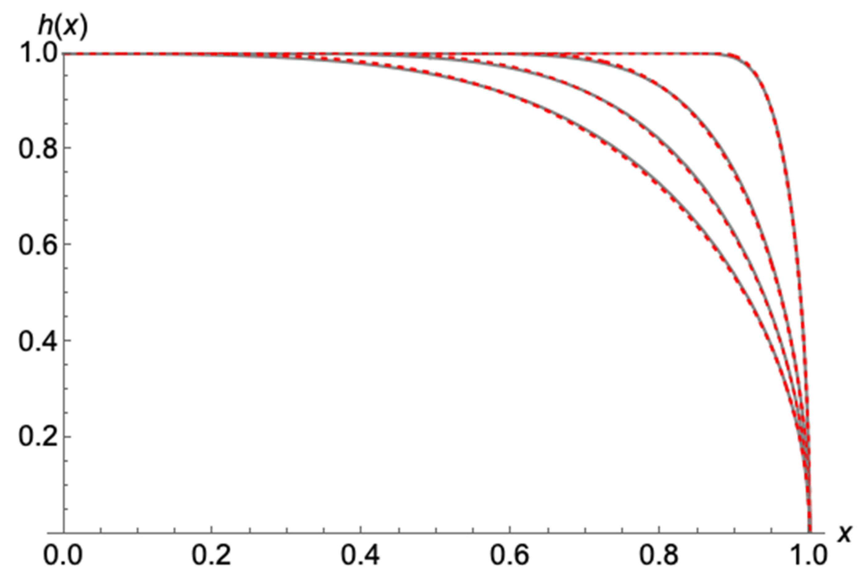
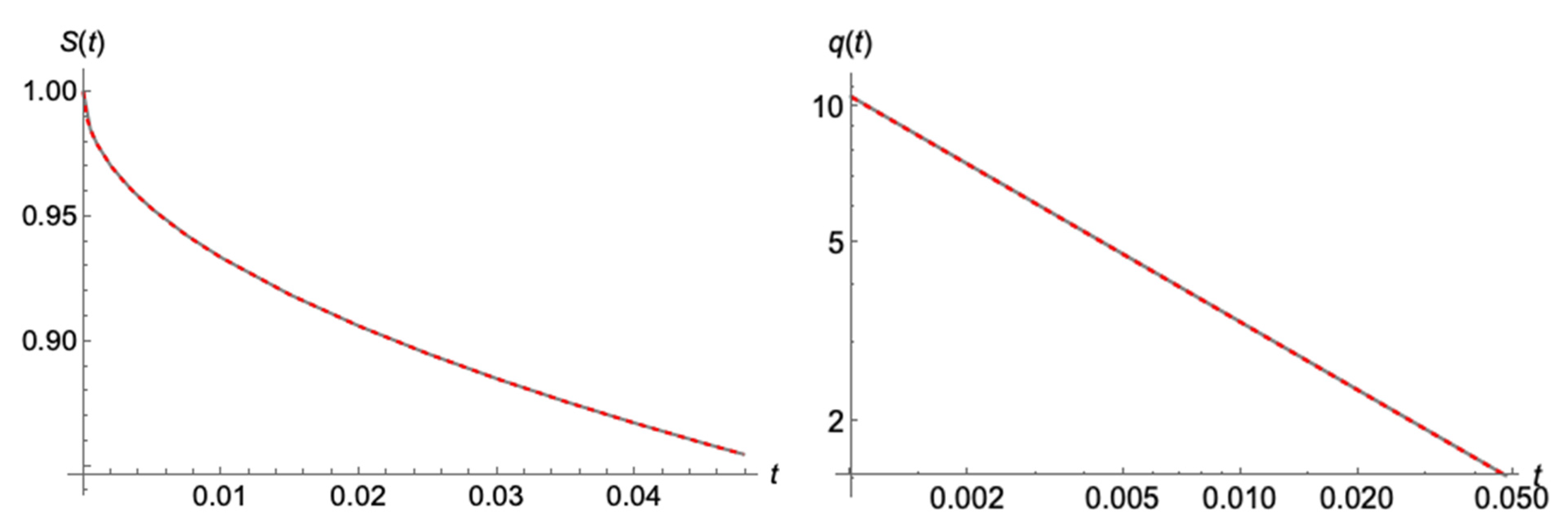
Applying the above, we present the evolution of the water depth (Figure 11) and the water storage and outflow (Figure 12) from the present “wave” model and the exact numerical solution of Boussinesq (3), starting from a horizontal initial profile and continuing up to time t = 0.0478442. The coincidence between the “wave” approximation (66) and the the Boussinesq Equation (3) is remarkable regarding the profile evolution (Figure 10), and becomes exact in the case of the mass balance and the outflow (Figure 12).

3.2.2. Later times

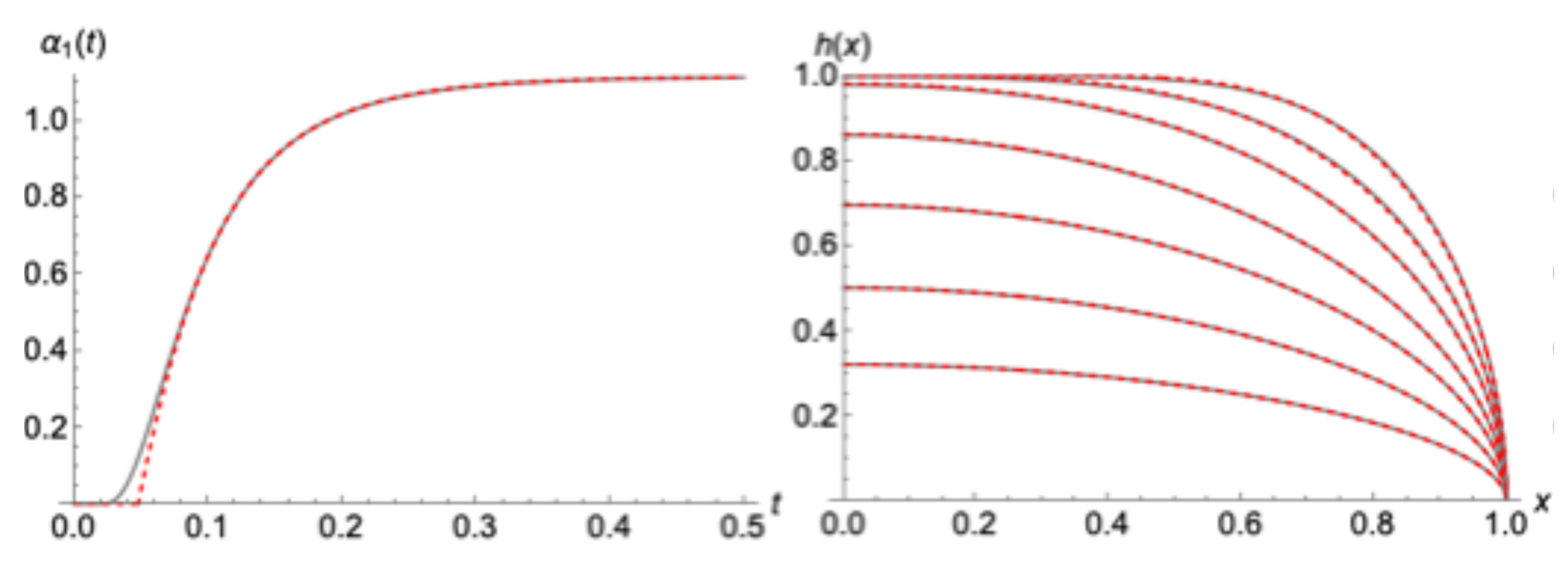
At the limitting time t_max = 0.0478442 when the wave reaches the upper end at x = 0, we make use of the new model (54) starting with the profile

s (x) = Φ (x)

from Equation (76) and continuing by solving numerically the system of Equations as analyzed in Section 3.1. As shown in Figure 13, even though parameter

a_{1} (t)

starts from a zero value in the modeled solution while the exact Boussinesq has proceeded (meaning that the head of the water table has already started decreasing slightly from 1, at t_max), both solutions match very fast. This matching drives also correctly the general pattern of the water table evolution, which is impressively captured.

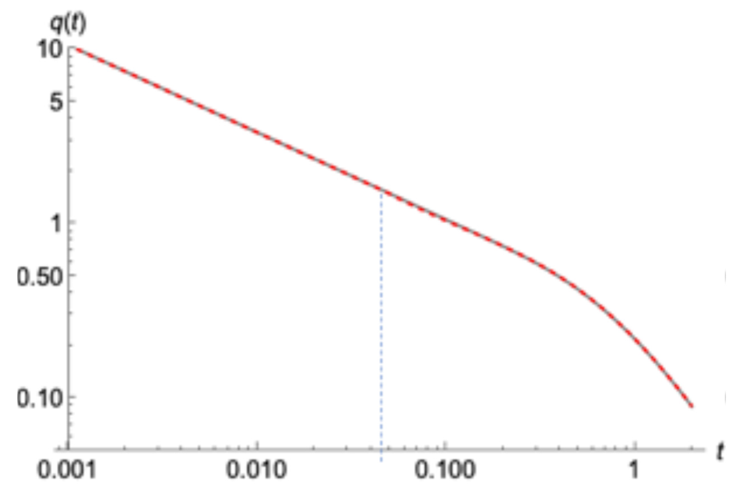
The outflow

q_{o} (t)

shows also a nice passage from the “wave” period of the solution to the new model (53) which matches almost perfectly the exact Boussinesq (Figure 14). Unlike the cases presented in Section 3.1, Boussinesq has now entered a more “mature” state satisfying the condition (65), thus the behavior of

\dot{q} (t)

is much smoother at the increment of time t = t_max. Such behavior is exactly what the new model can capture very accurately.

The above analysis together with the findings of the previous section regarding the initial “irregularity”, when recharging stops and pure drainage begins, paves the way of exploring the very early time of departing from any recharging period to drainage. Intuitively, one could guess departures of the form

q_{o} (t) = q_{o} (0) - k t^{z}

, 0 < z < 1, into the behavior of the outflow, but this is a matter of future research.

3.3. An Analytic Explicit Linear Approximation for the Solution of the New Model

In this last section, we approximate the non-linear system of Equations (53), (58) and (48) of the previously introduced and analyzed model with a linear form alowing for an analytical explicit solution for

a_{1} (t)

and the rest of the parameters, which proves to be accurate and well understandable.

Substituting into the mass balance main Equation (53)

- a_{1} S_{o} + h_{o}^{- 1} (S_{o, α_{1}} {\dot{a}}_{1} + S_{o, α_{2}} {\dot{a}}_{2}) = - (3 - 2 a_{1} + a_{2})

, of the model that was presented,

a_{2} = (0.9 a_{1}^{2} - h_{o}^{- 1} {\dot{a}}_{1})

/12 by Equation (58) and its first derivative

{\dot{a}}_{2}

, by

{\dot{a}}_{2} = \frac{(0.8 a_{1}^{} {\dot{a}}_{1} - h_{o}^{- 1} {\ddot{a}}_{1}^{})}{12}

(78)

we conclude with

a_{1} (S_{o} + 2 - \frac{0.9 a_{1}^{}}{12}) + {\dot{a}}_{1} h_{o}^{- 1} (\frac{1}{12} - S_{o, α_{1}} - S_{o, α_{2}} \frac{0.8 a_{1}^{}}{12}) + {\ddot{a}}_{1}^{} \frac{h_{o}^{- 2} S_{o, α_{2}}}{12} = 3

(79)

Then, dividing (79) with the multiplier of the term

a_{1}

(S_{o} + 2 - \frac{0.9 a_{1}^{}}{12})

, the mass balance Equation equivalently reads

a_{1} + {\dot{a}}_{1} \frac{h_{o}^{- 1} (\frac{1}{12} - S_{o, α_{1}} - S_{o, α_{2}} \frac{0.8 a_{1}^{}}{12})}{(S_{o} + 2 - \frac{0.9 a_{1}^{}}{12})} + {\ddot{a}}_{1}^{} \frac{\frac{h_{o}^{- 2} S_{o, α_{2}}}{12}}{(S_{o} + 2 - \frac{0.9 a_{1}^{}}{12})} = \frac{3}{(S_{o} + 2 - \frac{0.9 a_{1}^{}}{12})}

(80)

which obviously is a second order non-linear differential Equation of

a_{1} (t)

of the form

A {(a_{1}) \ddot{a}}_{1} + B (a_{1}) {\dot{a}}_{1} + a_{1} = C (a_{1})

(81)

When time derivatives vanish, Equations (79-81) yield

a_{1} = C (a_{1}) = \frac{3}{(S_{o} (a_{1}) + 2 - \frac{0.9 a_{1}^{}}{12})}

(82)

which is exactly the late time solution by Equation (60), defining the finite value of parameter

a_{1}

a_{1 f}

. Noting that in Equation (81) the function

C (a_{1})

does not vary strongly (i.e., the denominator typically varies in a range between 2.6 and 2.9 for most cases) we may nicely approximate

C (a_{1})

in Equation (81) with its finite value

C (a_{1}) = a_{1 f}

A {(a_{1}) \ddot{a}}_{1} + B (a_{1}) {\dot{a}}_{1} + a_{1} = a_{1 f}

(83)

assuring that

a_{1}

reaches the correct finite state

a_{1 f} .

In a rather crude way then, we simplify (83) even more, to the linear form

A {\ddot{a}}_{1} + B {\dot{a}}_{1} + a_{1} = a_{1 f}

(84)

where the time dependent non-linear terms

A (a_{1})

and

B (a_{1})

have been approximated with the constants A, B. Equation (84) is the linear approxiamtion of the exact Equation (80).

We saw, quite intuitevelly, that the best choice for the linerization constant values comes through demanding Equation (84) to satisfy the exact initial values of

a_{1} (0)

a_{10}

, and its derivatives at time zero,

{\overset{⃛}{a}}_{10}, {\ddot{a}}_{10}, {\dot{a}}_{10}

, as they are defined by the exact setting up. That way, Equation (84) incorporates correctly the initial and the finite behavior of the original non-linear system. Specifically, we demand A and B to satsisfy the system

A {\ddot{a}}_{10} + B {\dot{a}}_{10} + a_{10} = a_{1 f} A {\overset{⃛}{a}}_{10} + B {\ddot{a}}_{10} + {\dot{a}}_{10} = 0

(85)

and by solving, we conclude with the desirable values

A = \frac{a_{1 f} {\ddot{a}}_{10} - a_{10} {\ddot{a}}_{10} + {\dot{a}}_{10} {\dot{a}}_{10}}{{\ddot{a}}_{10}^{2} - {\overset{⃛}{a}}_{10} {\dot{a}}_{10}}, B = \frac{- {\dot{a}}_{10} - A {\overset{⃛}{a}}_{10}}{{\ddot{a}}_{10}}

(86)

Noting that

A

and

B

are possitive and that they differ by two orders of magnitude, the solution of (84) is always meaningful and can be straight forward expressed into the form

a_{1} (t) = a_{1 f} (1 - d_{1} e^{- w_{1} t} - d_{2} e^{- w_{2} t})

(87)

with

w_{1}

and

w_{2}

to be given by

w_{1} = \frac{B + \sqrt{B^{2} - 4 A}}{2 A}, w_{2} = \frac{B - \sqrt{B^{2} - 4 A}}{2 A}

(88)

and

d_{1}

d_{2}

d_{1} = \frac{B + \sqrt{B^{2} - 4 A}}{2 A}, d_{2} = 1 - d_{1} + \frac{a_{10}}{a_{1 f}}

(89)

After that The integration of Equation (87) over time gives through Equation (23) the evolution of the water table head at x = 0,

h_{o} (t)

, in the form

{h_{o}}^{- 1} (t) = 1 + a_{1 f} t + \frac{a_{1 f} d_{1}}{w_{1}} (e^{- w_{1} t} - 1) + \frac{a_{1 f} d_{2}}{w_{2}} (e^{- w_{2} t} - 1)

(90)

The remaining parameter

a_{2}

is calculated also by Equation (58) as

a_{2} = (0.9 a_{1}^{2} - h_{o}^{- 1} {\dot{a}}_{1})

/12. With these parameters we have completed the analytic approximation for the solution of the model and we may procced with the testing of its performance.

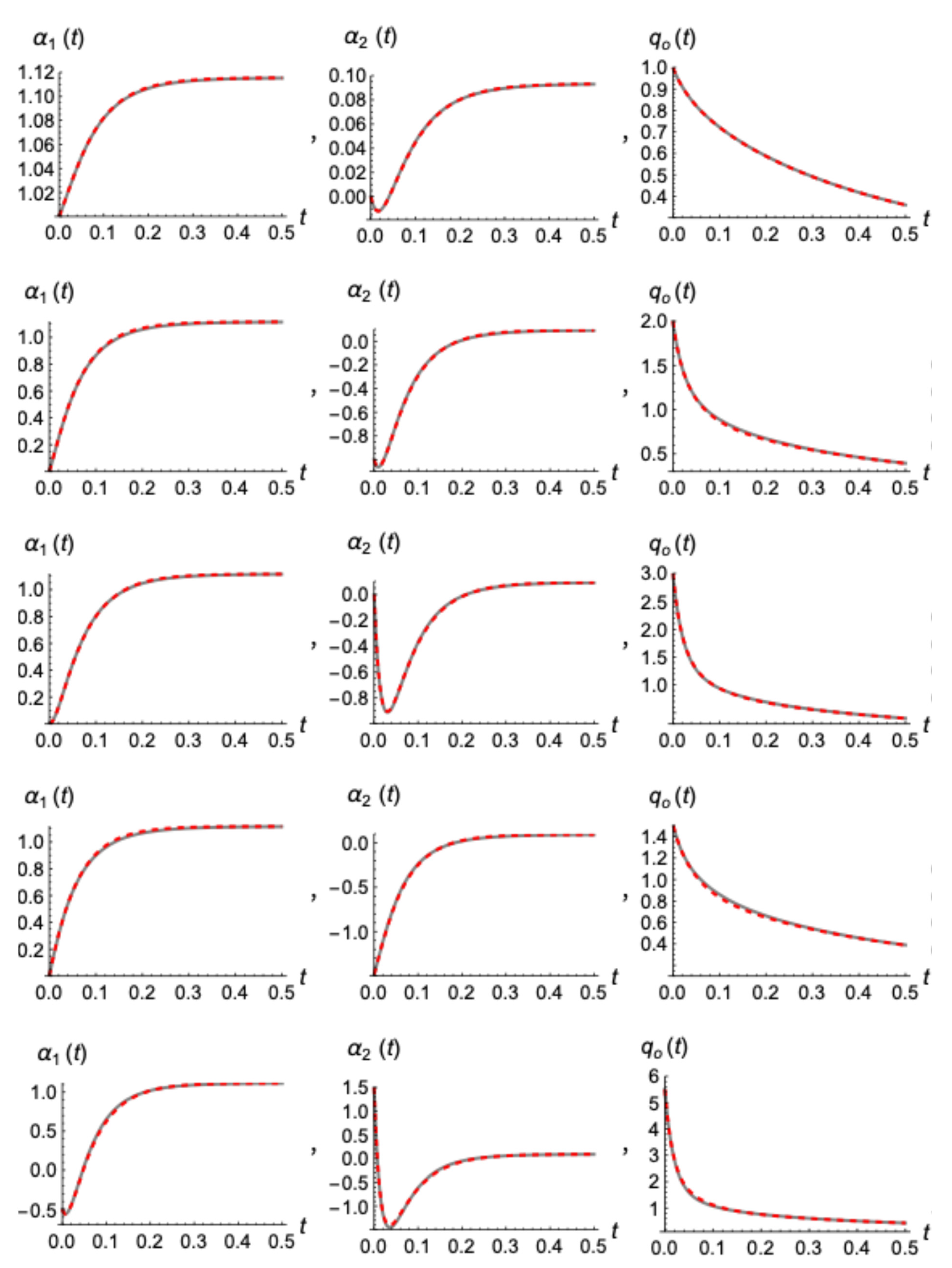
In the last Figure 15, we present the comparison between the evolutions of

a_{1} (t)

a_{2} (t)

and outflow,

q_{o} (t) = {h_{o}}^{2} (t) (3 - 2 a_{1} (t) + a_{2} (t))

as they are calculated numerically from the exact presented model in section 3.1, and analtically by its explicit linear approximation (89-90). We used all the previous initializations they have been discussed so far, corresponding to an initial

s (x, 0)

equal to,

\sqrt{1 - x^{2}}

\sqrt{1 - x^{4}}

\sqrt{1 - x^{6}}

and

\sqrt{1 - 1.5 x^{4} + 0.5 x^{6}}

. We have also added a more “exotic”, non-monotonous initial profile equal to

\sqrt{1 + 0.5 x^{2} + 1.5 x^{4} - 3 x^{6}}

. As it is shown, the performnce of the analytical expression (89) in estimating

a_{1} (t)

is overall very good with an accuracy of the order of 5 %₀ at its worst. This leads also to the accurate calculation of the rest of the parameters and especially the outflow, the most dificult one, to an accuracy of the order of ±1% at the worst case. That way, expressions (89) and (90) may serve as an easy and accurate representation both for the investigation and understanding of the drainage flow, as well as a modelling basis for handling more real cases.

Concluding, we should note that the same linearization idea can be applied in the case of a more accurate and detailed model of 8th order, by calculating three linearization parameters in that case

A {\overset{⃛}{a}}_{1} + B {\ddot{a}}_{1} + {C \dot{a}}_{1} + a_{1} = a_{1 f}

(91)

which yields a solution for

a_{1} (t)

of the form

a_{1} (t) = a_{1 f} (1 - d_{1} e^{- w_{1} t} - d_{2} e^{- w_{2} t} - d_{3} e^{- w_{3} t})

(92)

However, finding the proper linerization values for the constants A, B, C is much more complicated and needs special attention for satisfying stricter criteria for the solution to be well behaved.

4. Conclusions

We introduced and analyzed conceptual approximations of the Boussinesq Equation for horizontal unconfined aquifers during the pure drainage phase, without any reharge and zero-inflow conditions. We used a variety of methods, which include wave solution, variable separation and series expansion to constract a new model and explore its behavior and performance against the Boussinesq Equation and its exact (non-closed form) solution, at early and later times. The new model is based on the relations between the parameters defining the water table shape as they are implied by the Boussinesq Equation. To close the system of Equations the mass conservation pronciple were employed. The model proved to perform quite accuratelly for several initial water tables, becoming almost exact at the later times.

At the very early times there are some affordable deviations, from the exact Boussinesq, which were physically attributed to the different nature of recharging phase compared to the pure drainage period. As it was proven, in order to conform the imposed initial profile after recharge, Boussinesq concludes with a “violent” modification, resulting into a sudden change of outflow at an infinite rate. Modelling ideas in the form of a “wave” were discussed and applied to describe such rough changes, till the profile reaches a smoother shape that can be fed to the newlly proposed model, resulting in best accuracy.

The modeled non-linear forms were finally linearized concluding with explicit analytical expressions incorporating most of the basic characteristics regarding the evolution of the water table and the outflow from the exact Boussinesq Equation under different initial conditions.

The results from this research can be used as benchmarks for numerical modeling and serve as the basis for further theoretical development in groundwater hydrology with practical importance. Plausibly, these ideas could be further exploited to build simple, but effective, models for the very early behaviour of the drainage flow after any initial water table which was formed during the recharging period. Furthermore, they can be extended to describe the built-up phase during recharge as well, resulting into a complete tool. That will be the subject of future work of the authors.

References

Boussinesq, J. Essai sur la theorie des eaux courantes du mouvement nonpermanent des eaux souterraines. Acad. Sci. Inst. Fr. 1877, 23, 252–260. [Google Scholar]
Boussinesq, J. Recherches theoriques sur l’ecoulement des nappes d’eau infiltrees dans le sol et sur debit de sources. J. Math. Pures Appl. 1904, 10, 5–78. [Google Scholar]
Dupuit, J. Etudes Theoriques et Practiques sur le Mouvement des Eaux dans les Canaux Decouverts et a Travers les Terrains Permeables, 2nd ed.; Dunod: Paris, France, 1863. [Google Scholar]
Forchheimer, P. Über die Ergiebigkeit von Brunnen-Anlagen und Sickerschlitzen. Z. Architekt. Ing.-Ver. Hann. 1886, 32, 539–563. [Google Scholar]
Wooding, R.A.; Chapman, T.G. Groundwater flow over a sloping impermeable layer: 1. Application of the Dupuit-Forchheimer assumption. J. Geophys. Res. 1966, 71, 2895–2902. [Google Scholar] [CrossRef]
Barenblatt, G.I. On some unsteady fluid and gas motions in a porous medium. J. Appl. Math. Mech. 1952, 16, 67–78. [Google Scholar]
Polubarinova-Kochina, P.Y. Theory of Ground Water Movement; Princeton University Press: Princeton, NJ, USA, 1962. [Google Scholar]
Barenblatt, G.I.; Entov, V.M.; Ryzhik, V.M. Theory of Fluid Flows through Natural Rocks; Kluwer Academic Publishers: Dordrecht, The Netherlands, 1990. [Google Scholar]
Chen, Z.X.; Bodvarsson, G.S.; Witherspoon, P.A.; Yortsos, Y.C. An integral Equation formulation for the unconfined flow of groundwater with variable inlet conditions. Trans. Porous Media 1995, 18, 15–36. [Google Scholar] [CrossRef]
Lockington, D.A.; Parlange, J.Y.; Parlange, M.B.; Selker, J. Similarity solution of the Boussinesq Equation. Adv. Water Resour. 2000, 23, 725–729. [Google Scholar] [CrossRef]
Parlange, J.Y.; Hogarth, W.L.; Govindaraju, R.S.; Parlange, M.B.; Lockington, D. On an exact analytical solution of the Boussinesq Equation. Trans. Porous Media 2000, 39, 339–345. [Google Scholar] [CrossRef]
Telyakovskiy, A.S.; Braga, G.A.; Furtado, F. Approximate similarity solutions to the Boussinesq Equation. Adv. Water Resour. 2002, 25, 191–194. [Google Scholar] [CrossRef]
Pistiner, A. Similarity solution to unconfined flow in an aquifer. Trans. Porous Media 2008, 71, 265–272. [Google Scholar] [CrossRef]
Moutsopoulos, N. Solutions of the Boussinesq Equation subject to a nonlinear Robin boundary condition. Water Resour. Res. 2013, 49, 7–18. [Google Scholar] [CrossRef]
Basha, H.A. Traveling wave solution of the Boussinesq Equation for groundwater flow in horizontal aquifers. Water Resour. Res. 2013, 49, 1668–1679. [Google Scholar] [CrossRef]
Basha, H.A. Perturbation solutions of the Boussinesq Equation for horizontal flow in finite and semi-infinite aquifers. Adv. Water Resour. 2021, 155, 104016. [Google Scholar] [CrossRef]
Chor, T.; Ruiz de Zarate, A.; Dias, N.L. A generalized series solution for the Boussinesq Equation with constant boundary conditions. Water Resour. Res. 2019, 55, 3567–3575. [Google Scholar] [CrossRef]
Chor, T.; Dias, N.L.; Ruiz de Zárate, A. An exact series and improved numerical and approximate solutions for the Boussinesq Equation. Water Resour. Res. 2013, 49, 7380–7387. [Google Scholar] [CrossRef]
Tzimopoulos, C.; Papadopoulos, K.; Papadopoulos, B.; Samarinas, N.; Evangelides, C. Fuzzy solution of nonlinear Boussinesq Equation. J. Hydroinformatics 2022, 24, 1127–1147. [Google Scholar] [CrossRef]
Hayek, M. A simple and accurate closed-form analytical solution to the Boussinesq Equation for horizontal flow. Adv. Water Resour. 2024, 185, 104628. [Google Scholar] [CrossRef]
Tzimopoulos, C.; Samarinas, N.; Papadopoulos, K.; Evangelides, C. Fuzzy Analytical Solution for the Case of a semi-Infinite Unconfined Aquifer. Environ. Sci. Proc. 2023, 25, 70. [Google Scholar] [CrossRef]
Ceretani, A.; Falcini, F.; Garra, R. Exact solutions for the fractional nonlinear Boussinesq Equation. In Proceedings of the INdAM Workshop on Fractional Differential Equations: Modeling, Discretization, and Numerical Solvers, Singapore, 8 March 2023; Springer Nature: Singapore, 2023. [Google Scholar]
Akylas, E.; Gravanis, E.; Koussis, A.D. Quasi-steady flow in sloping aquifers. Water Resour. Res. 2015, 51, 9165–9181. [Google Scholar] [CrossRef]
Gravanis, E.; Akylas, E.; Sarris, E. 2024.
Gravanis, E.; Akylas, E. Early-time solution of the horizontal unconfined aquifer in the buildup phase. Water Resour. Res. 2017, 53, 8310–8326. [Google Scholar] [CrossRef]
Lockington, D.A. Response of unconfined aquifer to sudden change in boundary head. J. Irrig. Drain. Eng. 1997, 123, 24–27. [Google Scholar] [CrossRef]
Parlange, J. Y.; Stagnitti, F.; Heilig, A.; Szilagyi, J.; Parlange, M. B.; Steenhuis, T. S.; Hogarth, W. L.; Barry, D. A.; Li, L. Sudden drawdown and drainage of a horizontal aquifer. Water Resour. Res. 2001, 37, 2097–2101. [Google Scholar] [CrossRef]
Akylas, E.; Koussis, A.D. Response of sloping unconfined aquifer to stage changes in adjacent stream I. Theoretical analysis and derivation of system response functions. J. Hydrol. 2007, 338, 85–95. [Google Scholar] [CrossRef]
Koussis, A.D.; Akylas, E.; Mazi, K. Response of sloping unconfined aquifer to stage changes in adjacent stream II. Applications. J. Hydrol. 2007, 338, 73–84. [Google Scholar] [CrossRef]
Moutsopoulos, K.N. The analytical solution of the Boussinesq Equation for flow induced by a step change of the water table elevation revisited. Trans. Porous Med. 2010, 85, 919–940. [Google Scholar] [CrossRef]
Jiang, Q.; Tang, Y. A general approximate method for the groundwater response problem caused by water level variation. J. Hydrol. 2015, 529, 398–409. [Google Scholar] [CrossRef]

Figure 1. Cross-sectional schematic diagram of a horizontal soil layer, with constant and uniform hydraulic conditions during pure drainage period.

Figure 2. Cross-sectional schematic diagram of a horizontal soil layer, with constant and uniform hydraulic conditions during pure drainage period, with two well separated initial conditions. The steady state (9) after constant recharge of an infinite period (continuous line) and a uniform horizontal water table (10) (dashed line).

Figure 3. The gradual approach of

a_{1 f}

to its exact value given by Equation (36) as the order ν of the model (49) increases.

Figure 3. The gradual approach of

a_{1 f}

to its exact value given by Equation (36) as the order ν of the model (49) increases.

Figure 4. The perfect coincidence between the finite late time state calculated by the new model (red dashed line) through Equation (63) and the exact solution of the Boussinesq (gray line) Equation (34).

Figure 5. The nice coincidence between the present model’s (eq. 53) numerical application (red dashed lines), and the numerical solution of the exact Boussinesq Equation (gray lines), for drainage phase after an initial

h (x, 0) = \sqrt{1 - x^{2}}

, profile. The evolution histories for (from the upper left corner and continuing clockwise) the parameter

a_{1} (t)

, the water table head

h_{o} (t) = h (0, t)

, the outflow

q_{o} (t)

, and the water table

h (x, t)

(at times 0.025,0.05, 0.1, 0.25, 0.5, 1, 2).

h (x, 0) = \sqrt{1 - x^{2}}

, profile. The evolution histories for (from the upper left corner and continuing clockwise) the parameter

a_{1} (t)

, the water table head

h_{o} (t) = h (0, t)

, the outflow

q_{o} (t)

, and the water table

h (x, t)

(at times 0.025,0.05, 0.1, 0.25, 0.5, 1, 2).

Figure 6. As in Figure 5, for

h (x, 0) = \sqrt{1 - x^{4}}

, initially.

Figure 6. As in Figure 5, for

h (x, 0) = \sqrt{1 - x^{4}}

, initially.

Figure 7. As in Figure 5, for

h (x, 0) = \sqrt{1 - x^{6}}

, initially.

Figure 7. As in Figure 5, for

h (x, 0) = \sqrt{1 - x^{6}}

, initially.

Figure 8. Evolution of outflow

q_{o} (t)

at very early times from the present model’s (eq. 54) numerical application (red dashed lines), and the numerical solution of the exact Boussinesq Equation (gray lines), for drainage phase after initial profiles

h (x, 0) = \sqrt{1 - x^{2}}

\sqrt{1 - x^{4}}

and

\sqrt{1 - x^{6}}

(left to right).

Figure 8. Evolution of outflow

q_{o} (t)

h (x, 0) = \sqrt{1 - x^{2}}

\sqrt{1 - x^{4}}

and

\sqrt{1 - x^{6}}

(left to right).

Figure 9. Evolution of outflow

q_{o} (t)

h^{2} (x, 0) = 1 - x^{2} - \frac{1}{9} x^{4} + \frac{1}{9} x^{6} .

Figure 9. Evolution of outflow

q_{o} (t)

h^{2} (x, 0) = 1 - x^{2} - \frac{1}{9} x^{4} + \frac{1}{9} x^{6} .

Figure 10. Schematic representation of the water profile during the early drainage phase of the horizontal aquifer.

Figure 11. The agreement during the evolution of the water depth

h (x, t)

at early times between the full numerical solution (gray lines) and the present “wave” model (red dashed lines) at times 0.001, 0.01, 0.025, 0.0478442 (time increases downwards), starting from an initially horizontal profile.

Figure 11. The agreement during the evolution of the water depth

h (x, t)

Figure 12. The exact agreement of the evolution of the water storage

S (t) = \int_{0}^{1} h (x, t) d x

, and the outflow

q_{0} (t),

at early times between the exact numerical solution of Boussinesq (gray lines) and the present “wave” model, with

S (t) = 1 - 2 s_{1} \sqrt{t}

and

q (t) = s_{1} t^{- 1 / 2}

(red dashed lines), starting from an initially horizontal profile.

Figure 12. The exact agreement of the evolution of the water storage

S (t) = \int_{0}^{1} h (x, t) d x

, and the outflow

q_{0} (t),

at early times between the exact numerical solution of Boussinesq (gray lines) and the present “wave” model, with

S (t) = 1 - 2 s_{1} \sqrt{t}

and

q (t) = s_{1} t^{- 1 / 2}

(red dashed lines), starting from an initially horizontal profile.

Figure 13. The evolution histories of the parameter

a_{1} (t)

(left), and the water table

h (x, t)

(at times 0.025,0.05, 0.1, 0.25, 0.5, 1, 2), by the numerical solution of the exact Boussinesq Equation 3 (gray lines) and from the present wave approximation which is continued by the new model’s (eq. 53) numerical application (red dashed lines).

Figure 13. The evolution histories of the parameter

a_{1} (t)

(left), and the water table

h (x, t)

Figure 14. Evolution of the outflow from the full numerical solution (gray lines) and the combination of the “wave” model at early times and the 6th order model later on (red dashed lines). t_max is also shown, for better interpretation.

Figure 15. Comparison of the evolution of

a_{1} (t)

a_{2} (t)

and outflow,

q_{o} (t),

(right to left) by the numerical solution of the presented model (gray lines) and its analytic linear approximation (red dashed lines). Different initializations (up to down) correspond to

s (x, 0)

equal to:

\sqrt{1 - x^{2}}

\sqrt{1 - x^{4}}

\sqrt{1 - x^{6}}

\sqrt{1 - 1.5 x^{4} + 0.5 x^{6}}

and

\sqrt{1 + 0.5 x^{2} + 1.5 x^{4} - 3 x^{6}}

Figure 15. Comparison of the evolution of

a_{1} (t)

a_{2} (t)

and outflow,

q_{o} (t),

(right to left) by the numerical solution of the presented model (gray lines) and its analytic linear approximation (red dashed lines). Different initializations (up to down) correspond to

s (x, 0)

equal to:

\sqrt{1 - x^{2}}

\sqrt{1 - x^{4}}

\sqrt{1 - x^{6}}

\sqrt{1 - 1.5 x^{4} + 0.5 x^{6}}

and

\sqrt{1 + 0.5 x^{2} + 1.5 x^{4} - 3 x^{6}}

Disclaimer/Publisher’s Note: The statements, opinions and data contained in all publications are solely those of the individual author(s) and contributor(s) and not of MDPI and/or the editor(s). MDPI and/or the editor(s) disclaim responsibility for any injury to people or property resulting from any ideas, methods, instructions or products referred to in the content.

© 2024 by the authors. Licensee MDPI, Basel, Switzerland. This article is an open access article distributed under the terms and conditions of the Creative Commons Attribution (CC BY) license (http://creativecommons.org/licenses/by/4.0/).

Copyright: This open access article is published under a Creative Commons CC BY 4.0 license, which permit the free download, distribution, and reuse, provided that the author and preprint are cited in any reuse.

MDPI Initiatives

Important Links

Choose an area of interest and we will send you notifications of new preprints at your preferred frequency.

Disclaimer

Approximate Solutions for Horizontal Unconfined Aquifers during pure Drainage Phase

Abstract

Introduction

2. Pure Drainage Flow in Horizontal Unconfined Aquifers

2.1. Dimensionless Form of the Boussinesq Equation during Pure Drainage

2.2. Series Expansion and Late-Time Asymptotic Analysis of the Water Table during Pure Drainage

3. A New Model for the Drainage Phase of Horizontal Unconfined Aquifer

3.1. Analysis and Application of the New Model

3.2. The Case of a Sudden Drawdown from an Initially Horizontal Water Table

3.2.1. Early Time Approximation

3.2.2. Later times

3.3. An Analytic Explicit Linear Approximation for the Solution of the New Model

4. Conclusions

References

MDPI Initiatives

Important Links

Subscribe