Preprint
Article

The Impact of Restrictive Macroprudential Policies through Borrower-Targeted Instruments on Income Inequality: Evidence from a Bayesian Approach

Altmetrics

Downloads

57

Views

30

Comments

0

A peer-reviewed article of this preprint also exists.

This version is not peer-reviewed

Submitted:

28 August 2024

Posted:

12 September 2024

You are already at the latest version

Alerts
Abstract
The study used the data from emerging markets to examine the impact of restrictive macroprudential policies on income inequality from 2000–2019 using Bayesian panel vector autoregression and Bayesian panel dynamics generalized method of moments models. The chosen models are suitable for addressing multiple entity dynamics, accommodating a wide range of variables, handling dense parameterization, and optimizing formativeness and heterogeneous individualspecific factors. The empirical analysis utilized various macroprudential policy proxies and income inequality measures. The results show that when the central banks tighten systems using macroprudential policy instruments to sticker debt-to-income and financial instruments for lower-income borrowers (the bottom 40% of the income distribution) promote income inequality in these countries while reducing income inequality for high-income borrowers (the high 1 per-cent of the income distribution). The impact loan-to-value ratios were found to be insignificant in these countries. Fiscal policy through government expenditure and economic development reduces income inequality, while money supply and oil price shocks exacerbate it. The study suggests implementing a progressive debt-to-income (DTI) ratio system in emerging markets to ad-dress income inequality among lower-income borrowers. This would adjust DTI thresholds based on income brackets, allowing lenient credit access for lower-income borrowers while stricter limits for higher-income borrowers. This would improve financial stability and reduce income disparities. Additionally, targeted financial literacy programs and a petroleum-linked basic income program could be implemented to distribute oil revenue to lower-income households. Monetary Supply Stabilization Fund could also be established to maintain financial stability and prevent excessive inflation.
Keywords: 
Subject: Business, Economics and Management  -   Economics

1. Introduction

The Global Financial Crisis (GFC), triggered by U.S. housing bubbles, highlighted the need to manage housing and credit cycles for financial and macroeconomic stability. Conventional monetary policy during the financial crises become insufficient to address financial crises’ macroeconomic spillovers (Duca et al., 2020). Since the GFC, numerous countries have implemented macroprudential policies, particularly borrower-based tools like Loan-to-Value and Debt-to-Income regulations, to curb excessive credit expansion and increase borrowers’ resilience to house price shocks (FSB-IMF-BIS, 2011; IMF, 2014). The GFC significantly impacted many emerging economies, leading to a lack of recovery. Unemployment increased in some countries before improving, exacerbated income and wealth inequality, which has been rising since the 1980s, as noted by Piketty (2014), Atkinson (2014) and Sarfati (2015) among others.
Given that it has been noted in the literature, as found in the study by Duca et al. (2020), numerous countries have adopted macroprudential policies, and Piketty (2014), among others, noted that income inequality has been on the rise, which is claimed to be contributed by the GFC. Therefore, the current study seeks to examine whether the borrower-based toolkit is more severe in contributing to income inequality in the adopted countries. This is supported by the findings published by Bernanke (2015) and others, who contend that more research is necessary to fully understand and quantify the effects of monetary policy on income and wealth inequality. They also stress the importance of identifying the channels through which monetary policies may have distributive effects.
A growing literature explores the impact of macroprudential policy on credit growth, particularly household credit growth, and its linkages to housing boom-bust cycles. These studies finds that macroprudential instruments effectively decreases credit growth notable household credit growth (Alpanda and Zubiary, 2017; Cerutti et al., 2017). While some studies suggest that macroprudential instruments effectively reduce credit growth, mixed evidence exists for their effects on curbing house price inflation (Jacome and Mitra, 2015; Kuttner and Shim, 2016; Akinci and Olmstead-Rumsey, 2018; Alam et al., 2019). While other the other side the literature on the impact of macroprudential and income inequality sims to be contradictory as some find the evidence of the re-distributional effects of macroprudential policy (Zinman, 2010; Carpantier et al., 2017; Frost & van Stralen, 2018; Georgescu & Martin, 2022).
Tzur-Ilan (2016), analysing the impact in Israel and Acharya et al. (2017) in Ireland, argue that borrower-related macroprudential instruments increase wealth inequality by making poorer borrowers more vulnerable. Carpantier et al. (2018) argue that macroprudential policies can increase wealth inequality through the LTV cap. Kostantinou et al. (2021) also documented that these policies create income inequality. Andries and Melnic (2019) argue that macroprudential policies affect income and wealth inequality through the level of economic development.
The distributional effects of macroprudential policies have not been extensively studied in empirical literature, with limited evidence and a focus on advanced economies. Furthermore, the research faces limitations due, firstly, to the heterogeneity of policies, their financial implications, and varying economics, making it challenging to provide conclusive answers. Second, the time period for the implementation of these instruments is short, since this policy became intensively used during and after the 2007 financial crisis and further, their recent origin. Third, it might be difficult to unravel the effects of macroprudential policies on the effects of other policies (monetary and fiscal), as well as any policy-driven changes in the financial sector. Therefore, much research is required in order to shed more light on the impact of macroprudential policies on macroeconomic indicators. This research aims to clarify the subject meter in emerging countries’ perspectives on policy programs, which are still in their early stages and have limited documentation, especially in low-income countries. Concerns have arisen regarding potential economic consequences, such as restricting credit and financial access and causing long-term and short-term output costs (Arregui et al., 2013). The IMF unveiled another concern that constitutes this paper: that these policies may increase inequality by favouring more well-off segments of the population, undermining progress in education and health in LIDC and emerging countries (IMF, 2014c). Apart from inequality concerns, mounting research suggests that inequality may be a significant determinant of financial instability by fuelling financial imbalances on credit markets (Rajan, 2010; Zungu and Greyling, 2023).
Considering these limitations, the current study seeks to contribute to the current literature by taking a different approach from the one that exists in the literature. Following the approach taken by Alter et al. (2018), this study investigated the impact of macroprudential policy on income inequality using a panel data for 15 emerging markets covering the period 2000-2019, using the Bayesian Panel Vector Autoregressive (BPVAR) and Bayesian Generalised Method of Moments (BGMM) with other two single equations models for robustness: the fixed effect (FF) and fully modified ordinary least squares (FMOLS). The focus is on the two borrowers: the lower and higher borrower. This would then be linked with two macroprudential instruments such as the debt-to-income ratio and the loan-to-value ratio. This then would be define as follows; the debt-to-income ratio of lower-income borrowers (the bottom 40 percent of the income distribution) and the debt-to-income ratio of high-income borrowers (the high 1 percent of the income distribution), as well as the loan-to-value ratio of lower-income borrowers (the bottom 40 percent of the income distribution) and the loan-to-value ratio of high-income borrowers (the high 1 percent of the income distribution).

2. Theoretical Framework

2.1. Theoretical Channels of Macroprudential Policy and Income Inequality

The initial goal of macroprudential regulations was to address financial stability issues by decreasing credit risk and controlling credit cycles (Tenreyro & Thwaites, 2016). Macroprudential regulations increase credit costs by constraining credit availability, affecting income and wealth distribution. Little theoretical research exists on this topic, but models like bank capital requirements, asset-based ratios, and collateral restrictions are often used to examine the impact of macroprudential tools on the housing market.
The research on the impact of macroprudential regulations on income and wealth inequality highlights the importance of long-term loan (LTV) limits, which directly affect credit availability and income disparity. LTV limitations can make credit more expensive and difficult to obtain, particularly for low-wealth families. This can lead to them purchasing less expensive properties or potentially putting property ownership out of their reach. Carpantier et al. (2017) highlight the different impacts of LTV limitations on borrowers and mortgage holders. Macroprudential policies can improve welfare by lowering household debt, reducing the likelihood of future defaults, and providing financial stability to borrowers (Rubio & Carrasco-Gallego, 2014). This decreases wealth inequality by increasing the net worth of low-income families. However, stricter credit conditions and reduced LTV caps can be detrimental to LTV-type lower households, leading to a reconsideration of their default risk and the risk of unduly high mortgage debt if house prices fall. Households with moderate or low incomes may find themselves overwhelmed by mortgage payments exceeding property values, reducing their net worth, and increasing wealth disparity (Punzi & Rabitsch, 2018).
Punzi and Rabitsch (2018) and Rubio and Unsal (2017) conducted research on macroprudential policies involving collateral requirements in low- and emerging-income countries. They found that a passive strategy of increasing collateral needs leads to a lower steady-state level of production, resulting in income inequality. Entrepreneurs were found to be the most affected, as more stringent collateral requirements limited their access to credit, resulting in decreased income, consumption, and output. Stiglitz (2015) argued that while lowering collateral requirements may not always improve economic efficiency, it does raise income inequality. A decrease in loan collateral leads to higher capital gains and land prices for landowners, while banks profit from additional lending. High-income households often bear the brunt of the consequences of capital requirements, according to a study by Mendicino et al. (2018). The study uses a microfounded, medium-scale, general equilibrium model to assess the distributional impact of capital requirements following Clerc et al. (2015) model. The model considers the fraction of assets that depreciate. Banks receive government subsidies when the failure probability is positive, creating a moral hazard. Higher capital requirements minimize inefficiencies, such as subsidizing deposit insurance, which improves the well-being of savers.
Higher capital requirements can hinder financial intermediation and negatively impact borrowers’ wellbeing. They are Pareto-improving up to a point and redistributive thereafter (Mendicino et al., 2018). When capital requirements begin at modest levels, both savers and borrowers benefit from growth. Savers benefit from lower financial fragility, while borrowers suffer due to decreased bank default costs and higher loan interest rates. Optimal capital requirements optimize borrowers’ long-term wellbeing. Banks must meet these requirements to avoid defaults. Households borrow from banks to acquire homes, while companies borrow to support investment. Banks may fail if loan earnings are inadequate to repay deposits, as intermediaries support themselves with equity and insured deposits. The trade-off between savers’ and borrowers’ wellbeing is crucial in capital requirements.

2.1.1. Transmission Channels

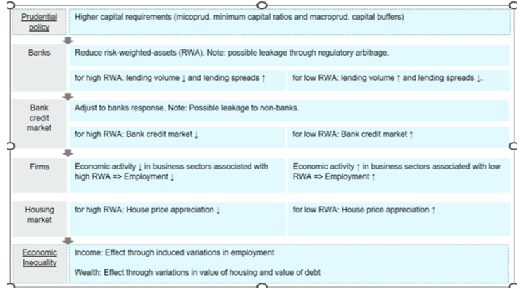
Prudential policies can impact economic inequality through two types of instruments: borrower-related instruments and capital-related instruments. Borrower-related instruments, such as the LTV ratio and DTI ratio, demand higher capital ratios from banks. Capital-related instruments, such as microprudential minimum capital ratios and macroprudential capital buffers, force banks to maintain higher capital ratios.
Table 1. Transmission mechanism for capital related policies.
Preprints 116560 i001
The transmission mechanism involves banks, the credit market, asset market, aggregate economic activity, and households. When banks face high capital requirements due to these instruments, they may modify their lending to reduce the total risk-weighted assets (RWA). The adjustment to changes in the bank credit market involves lowering lending volume and raising lending spreads for high-risk assets or increasing lending volume and decreasing lending spreads for low-risk assets (Martynova, 2015). However, regulatory arbitrage can lead to leakages. The bank credit market contracts for high-risk-weighted assets and expands for low-risk-weighted assets. Interventions that increase the cost of bank capital can slow loan growth. As the bank credit market contracts, there may be leakage to non-bank credit markets, such as shadow banking.

2.2. Review of Empirical Literature

This section discusses empirical literature on the same subject. After scrutinizing the empirical literature on this subject, the researcher revealed five relevant empirical papers that examine the impact of macroprudential policy on inequality (Zinman, 2010; Tzur-Ilan, 2016; Frost and van Stralen, 2017; Acharya et al., 2017; Carpantier et al., 2018). The study by Zinman (2010) investigated the wealth and consumption effects of macroprudential measures in the state of Oregon in the USA. The empirical evidence shows that macroprudential policies have a redistributive effect on wealth inequality. The argument was taken further by Tzur-Ilan (2016) following a borrower-related argument using a macro-analytical framework to examine the introduction effect of the LTV limit in Israel. The empirical findings show that: (i) borrowers buy cheaper houses in lower-quality neighborhoods; and (ii) the demand for consumer credit will increase significantly as mortgage rates rise. As consumer credit is a form of unsecured debt associated with higher rates, borrowers increase the economy’s overall exposure to the risk of a recession and unemployment. The results support the argument that LTV macroprudential instruments are likely to make fewer wealthy borrowers more vulnerable.
Furthermore, Acharya et al. (2017) studied the effect of the introduction of DTI and LTV caps in Ireland on residential mortgage credit. The author argues that the introduction of borrower-related instruments influences banks to (i) reduce the rate charged to high-income households who buy expensive properties, which then (ii) increases their mortgages to the high-income quintile, whilst issuance to the bottom-income quintile does not change. The results of this study support the argument that borrower-related macroprudential instruments make the wealthy group wealthier, thus increasing wealth inequality. Frost and van Stralen (2017) used the database of Cerutti et al. (2016) for 69 countries over the time span 2000–2013 to investigate the causal relationship between macroprudential instruments and the Gini coefficients of net and market inequality.
The findings reveal evidence for the redistributive effects of macroprudential policy. The finding shows that tighter measures such as higher reserve requirements and, LTV caps, as well as concentration and interbank exposure limits, increase income inequality. The argument was taken further by Carpantier et al. (2018) doing a household survey in 12 European Area countries employing HFCS data. The author found that caps on LVT ratios may reduce wealth inequality in the sense that households find it tougher to get a mortgage, which results in low indebtedness which pushes wealth inequality low.
According to emerging empirical evidence, inequality may be a major driver of financial fragility by exacerbated financial imbalances on credit markets (Rajan, 2010; Hauner, 2020). The argument is that high-income inequality forces middle and low-income households to borrow more than they reasonably should in order to maintain the relative levels, which leads to excess borrowing (credit bubbles), which in turn leads to financial crises. Recent evidence suggests that macroprudental measures applied to foster financial stability, might have an impact on wealth and income inequality (Carpantier et al., 2017; Mendicino et al., 2018).
Many studies, on the other hand, show that unconventional monetary policy is the primary determinant of income and wealth inequality (Saiki and Frost, 2014; Bivens, 2015; Rupprecht, 2018; Davityan, 2018; Guerello, 2018; Lenza and Slac alek, 2018; Taghizadeh-Hesary et al., 2018; Lenza and Slacalek, 2019). To the best of my knowledge, Saiki and Frost (2014) were the first authors to explore the impact of UMPs on income distribution using semi-aggregated household survey data for Japan. Today, a large number of empirical studies have studied the impact of UMPs on income inequality in various economies. Rupprecht (2020) studied the impact of UMPs on financial wealth and household income across different Euro area countries. The findings confirmed the UMP’s widening household income and financial wealth. The finding was further supported by Davityan (2018) in a case involving the US, and Casiraghi et al. (2018) in the case of Italy, using microdata. The findings confirmed that UMPs are not the drivers of an increase in inequality in Italy. Doepke et al. (2015) studied the same subject for the US. The findings yielded that UMPs benefit middle-class borrowers with mortgages but hurt wealthy pensioners with nominal savings. More recently, the study by Lenza and Slacalek (2019) in the Euro area confirmed that UMPs did not increase inequality as a result of job creation and wage increase effects.
Other studies believe that UMPs have an impact on inequality and wealth distribution through the channels of earning heterogeneity and income composition. The scholars who believe in the earning heterogeneity channel argue that quantitative easing stimulates economic activity and wage growth, which then creates more job opportunities. As a result, wage growth and income inequality have been stimulated. This channel’s empirical evidence is reported in studies conducted by Bivens (2015) for the United States, Casiraghi et al. (2018) for Italy, and Guerello, 2018; Lenza and Slac alek, 2018) for the Eurozone. While some schools of thought that believe in income-composition channels argue that UMPs are the drivers of an increase in income inequality by boosting the capital income of the upper class, asset prices and income inequality increase. The evidence that supports the income-composition channel is documented by Taghizadeh-Hesary et al. (2018) for Japan, Juan-Francisco et al. (2018) for the USA, and Mumtaz and Theophilopoulou (2017) for the UK.
The overall effect of income-composition and earning heterogeneity channels determines the UMPs on income inequality (Saiki and Frost, 2014; Inui et al., 2017; Casiraghi et al., 2018. The empirical findings on the subject are mixed and not clear. The impact of both macroprudential policies and monetary policy through unconventional monetary policy varies depending on the examined policy measure, the distributional channel, as well as on the economic structure of the country studied and the characteristics of household income. Therefore, more investigation is required into understanding the impact of macroprudential policies and monetary policy through unconventional monetary policy. However, this study targeted African countries.

3. Research Methods and Data Used for the Study

To achieve the objective of this study, the researcher used a panel data of 15 emerging markets covering the period 2000–2019. This study adopted variables that were suggested in the literature. The researcher used the Gini coefficient at market income (inq) obtained from the Standardized World Income Inequality Database (Solt, 2020) to capture income inequality. While for robustness and variable sensetivity the author used two variables to measure income inequality in the empirical analysis: the pre-tax income held by the top 10% (dincPTI10) and the pre-tax income held by the top 1% (dincPTI10) collected from the World Inequality Database (Alvaredo et al., 2018). The dates for the period were chosen on the grounds of data availability. This study examines the impact of macroprudential policy on income inequality, focusing on lower and higher-income borrowers. Following the study by Alter, Feng and Valckx (2018), the current chapter uses three macroprudential instruments: the financial instrument, the DTI ratio, and the LTV ratio. The financial instrument (FNCE) was calculated based on DP + CTC + LEV + SIFI + INTER + CONC + FC + RR_REV + CG + TAX (Cerutti et al., 2017), while DTI and LTV are defined as stated in Section 3.2: the DTI ratio of lower-income borrowers (the bottom 40% of the income distribution) and high-income borrowers (the top 1% of the income distribution), as well as the LTV ratio of lower-income borrowers (the bottom 40% of the income distribution) and high-income borrowers (the top 1% of the income distribution). The LTV ratios are properly defined as restrictions to LTV, used as a strictly enforced cap on new loans, as opposed to a supervisory guideline or merely a determinant of risk weights, while DTI ratios constrain household indebtedness by enforcing or encouraging a limit (Cerutti et al., 2017). One of the concerns, as stated in Section 3.2, is that "it might be difficult to unravel the effects of macroprudential policies on the effects of other policies (monetary and fiscal), as well as any policy-driven changes in the financial sector". Therefore, we control both fiscal and monetary policy in the system.
While the model used in this study controls for a fiscal policy (GE) shock through government spending as a percentage of GDP, it is well documented that government spending plays a crucial role in redistribution by reducing income inequality (Zungu et al. 2022). While the researcher controls for a monetary policy shock through Broad Money Supply (M2 over GDP) (BMS) following the argument by Elekdag and Wu (2011: p.9), the interest rate alone may represent the level of global financial liquidity accurately, especially in an unconventional monetary policy environment. Therefore, to address this issue, the researcher adopted the interest rate series as a metric of broad money supply. Another concern on the list is the literature, as the studies by Adarov and Tchaidze (2011), among others, argue that the overall level of economic development captured by GDP per capita (GDPp) is a major predictor of credit availability and financial progress. Economic development was then controlled for, as well as the pro-cyclicality of credit, following Borio et al. (2001). Lastly, neglecting the oil-price (OIL price) effect on the system might have serious negative implications for the results of the study. Therefore, the oil-price spillover effect on the subject was also controlled for. For model sensitivity this study controlled for inflation (INFL). The variables were sourced from different databases, such as the World Development Indicators and the Cerutti data (Cerutti et al., 2017).

3.1. Bayesian Panel Vector Autoregressive (BPVAR) Model

The study used the BPVAR technique established by Canova and Ciccarelli (2004), which is based on Bayesian shrinkage estimators and predictors advocated by Zellner and Hong (1989) and Zellner, Hong, and Min (1991), to analyse the interactions between macroeconomic factors and individual nation heterogeneity. This panel VAR approach allows for variance in the data’s temporal and cross-sectional dimensions, inferring dynamic correlations between variables and allowing for endogenous covariates. The study focused on a small number of variables reflecting the dynamics of major macroeconomic factors. A PVAR framework was used to pool all nations in the sample for joint estimation, enhancing estimate quality by increasing the cross-sectional dimension. Recent models have been developed to infer and evaluate idiosyncratic shocks within the PVAR framework, accounting for additional transmitted shocks and spillover effects (Crespo-Cuaresma & Fernandez-Amadorb, 2013; Reinhart & Rogoff, 2009; Ciccarelli & Rebucci, 2007). Formalizing, given N countries indexed i = 1 ;   2 ;   ; N and time t = 1 ;   2 ;   ;   T , the model is defined as follows:
X i t = μ i + Θ L X i t + u i t
where X i t is the vector consisting of seven endogenous variables, i.e., income inequality, the financial instrument, the DTI ratio, the LTV ratio, government spending, broad money supply, economic development and oil price; L , μ i is the vector of time-invariant country fixed effects, Θ L is a matrix polynomial in the lag operator and   u i t is the error term. The specified variable setup represents a most parsimonious model allowing for efficient estimation in light of the relatively small number of observations. The study uses the Bayesian PVAR estimator to solve over-parametrisation difficulties and to use Bayesian shrinkage due to the small sample size. The MATLAB version of the ECB’s Bayesian Estimate, Analysis, and Regression (BEAR) toolbox is used as described in Dieppe et al. (2016), handling model parameters as random variables with underlying probability distributions. This methodological approach combines previous knowledge about model parameters and updates probability distributions based on observed data. The study uses a typical Normal-Wishart prior, default hyperparameter settings, and the BPVAR pooled estimator, which is the Bayesian equivalent of the mean-group estimator and suggests homogenous coefficients across nations, to infer dynamic reactions from shocks of interest. The study’s goal is to infer dynamic reactions from shocks of interest.
The modelling method assumes that the residual vector u i t is independent and uniformly distributed. However, this condition is often violated due to the variance-covariance matrix containing mistakes. To isolate shocks to VAR errors, the residuals must be decomposed to become orthogonal. Sims (1980) proposed the Cholesky decomposition of the residual variance-covariance matrix, which ensures shock orthogonalisation. Variables that arrive first impact variables that come after them concurrently and with a latency, while variables that come last only affect those that come before them with a lag (Love & Zicchino 2006). The study uses the Cholesky factorisation algorithm to compute orthogonalised impulse-response functions (IRFs) and forecast error-variance decomposition (FEVD) after estimating the Bayesian PVAR model to track the influence of macroprudential shocks on income inequality. The variables used for Cholesky decomposition are ordered similarly to the PVAR specification, with X i t = [income inequality, financial instrument, DTI ratio, LTV ratio, government expenditure, broad money supply, economic development, and oil price].This ordering means that variables lower in the ordering may have an effect on variables higher in the ordering.

3.2. The Two-Step System Dynamic Panel Data: BGMM: Bayesian Framework Setup

To support the results of the BPVAR model, this study adopted the Bayesian Generalized Method of Moments for producing and quantifying the magnitude of the impact of macroprudential policy instruments on income inequality. The general model is as follows:
Y i = r = 1 ρ θ k X i t + ϵ i
where Y i is a N · 1 vector denoting the variable of interest, with i = 1 , 2 , . . . , N , X i t = X i 1 ,   X i 2 , . . , X i m is a [ N   · m ] matrix including a few, or a large set of continuous and/or discrete covariates, with k = 1 ,   2 ,   .   .   .   ,   m , θ k = θ 1 ,   θ 2 , . . , θ m is a k   ·   1 vector of unknown regression coefficients, and ǫ i   N ( 0 , σ 2   u ) is a N   ·   1 vector of disturbances, with σ to be an unknown positive scalar. Here, for simplicity, the constant term is dropped, and it is assumed that the error component is independent and identically distributed ( i .   i . d . ) and homoskedastic.

3.2.1. Dynamic Panel Data with GMME Estimators Setup

The baseline where the Bayesian setup is combined with the GMM is presented as follows:
Y i t = δ i + r = 1 ρ γ r W i t r + i = 0 λ ξ = 1 k θ l ξ X i t l ξ + u i t
where Y i t is a N T   · 1 vector of outcomes, δ i is a N · 1 heterogeneous intercept, W i t r is a N T   · 1 vector of predetermined variables, W i t r , ξ   i s a NT ·κ matrix containing continuous/discrete endogenous variables, with l = 0, 1, 2, …, λ ,   r = 1, 2, …, ρ denotes generic Auto-Regressive (AR) orders for the predetermined variables,   γ r and θ ˜   λ ξ are the autoregressive coefficients to be estimated for each i and couple of ( i   , ξ ), with ˜ λ = 1 ,   .   .   .   , λ, and u i t   i   . i   . d . N ( 0 , σ 2   u ) is a N T   ·   1 vector of unpredictable shock (or idiosyncratic error term), with E( u i t ) = 0 and E( u i t · u j s ) = σ 2   u   i f   i = j   a n d   t = s , and E( u i t · u j s ) = 0 otherwise.
Here, some considerations are in order: (i ) the predetermined variables contain the lagged values of the outcomes Y i t and lags of heterogeneous individual-specific factors; (ii ) the δ i s denote cross-unit heterogeneity affecting the outcomes Y i t ; (iii ) a correlated random-effects approach is adopted in which the δi s are treated as random variables and possibly correlated with some of the covariates within the system; (iv) the roots of r ( B ) = 0   a n d   ˜ l ( B ) = 0 lie outside the unit circle so that the AR processes implicit in model [2] are stationarities, with ˜ l = 1 ,   2 ,   .   .   .   ,   ˜ λ denoting generic AR orders for the endogenous variables and B referring to the lag operator; and (v) the instruments are fitted values from autoregressive parameters based on all the available lags of time-varying variables and their causal interactions. The researcher then further employs single-equation methods such as fixed effect (FE), and fully modified ordinary least squares (FMOLS) to further validate the results of the BVAR and BGMM.

4. Analysis of Empirical Results

The study uses the BEAR toolbox to estimate the BPVAR model for 15 emerging markets from 2000-2019, focusing on the dynamic impact of macroprudential policy on income inequality and its spillover effect. Bayesian GMM technique is used to quantify the impact, while single equation methods like FE, and FMOLS estimation are employed. Impulse Response Functions and Cholesky variance decomposition are used to trace the responsiveness of each endogenous variable to innovative shocks. The descriptive statistics for each variable are included in Table 2, and the findings of the line and autocorrelation diagnostic plots are shown in Figure A1 in the Appendix A. According to descriptive statistics, for all variables of income inequality, average income inequality captured by SWIID, incPalma-ratio, incPT10, and incPT1 in these countries is around 48.29, 48.29, 50.54, and 45.39 percent, and macroprudential policies captured by DTI, LTV, and FNCE in these countries are around 19.71, 70.23, and 48.03 percent. All of the variables are found to be negatively skewed, as reported.
All the variables had kurtosis values within the required range of 2 to 3 percent, contradicting the alternative normality hypothesis. The probability values of the Jarque-Bera tests for all variables were less than 10%, suggesting country-specific factors may be responsible for the rejection of the normal distribution hypothesis. We use panel data stationarity tests to avoid deceptive parameter estimates. The Im-Pesaran-Shin test developed by Im et al. (2003) and the Harris-Tzavalis test by Harris-Tzavalis (1999) are used to assess stationarity.
Table 3 summarizes the test, showing that all variables except YOU and ADS are non-stationary in levels and stationery after the first difference. The study employs I(1) variables, except for two stated variables, I(0). This study validated variables through cointegration and cross-sectional independence using Pedroni cointegration (Pesaran 2004), cross-sectional dependence test statistics (Friedman 1937), and Frees’ (1995) test data, as shown in Table 2.The null hypothesis that there is no cointegration and cross-sectional reliance in variables is significantly rejected by the Pedroni cointegration test and three cross-sectional reliance tests.

4.1. The Result of the BPVAR Model

As noted earlier, we use BPVAR to examine the dynamic impact of macroprudential policy measures on income inequality in emerging countries, as well as to investigate whether the policy shock is persistent over time, covering the period 2000–2019. The IRFs generated from the BPVAR are shown in Figure 1, where the coefficients for the dynamic impact of macroprudential policy instruments on income inequality have been given a tighter hierarchical priors distribution. The shaded areas represent the 16% and 84% credible sets, respectively. Figure 1, Figure 2 and Figure 3 show the response of income inequality to the restrictions on the LTV ratio, DTI ratio, and financial ratio of the lower-income borrowers (bottom 40% of the income distribution) and the high-income borrowers (top 1% of the income distribution), following the approach documented by Alter et al. (2018) in the case of macroprudential policy and economic growth. The argument for the study, to analyze the shock of macroprudential policy based on the level of income distribution, is to trace which group of income suffers the most when there are restrictions on the adopted macroprudential policy measures. Figure 1 in Column 1 shows that when the CB tightens the system by using macroprudential policy instruments to restrict the DTI ratio of lower-income borrowers (the bottom 40% of the income distribution), it appears to be more instrumental in promoting income inequality in the bottom 40% of the income distribution in these countries, following a one percent standard deviation shock to the DTI ratio of lower-income borrowers (the bottom 40% of the income distribution) and attaining a maximum impact of 0.15 five years after the shock. The results further show that the impact is persistent over time.
On the other hand, in Column 2, based on the restrictions on the DTI ratio of the high-income borrowers (the top 1% of the income distribution), the results of this study are very interesting, as the study documents that income inequality responds negatively following a one percent standard deviation shock on the DTI ratio of the high-income borrowers (the top 1% of the income distribution), achieving a maximum effect of 0.13 five years later, then converging after two years, reverting to the steady state area, and dying. The results further show that the impact is persistent over time.
These findings are in line with the results documented by Tzur-Ilan (2016), who stress that LTV macroprudential instruments are likely to make less wealthy borrowers more vulnerable, while the studies by Acharya et al. (2017) and Frost and van Stralen (2017) support the notion that borrower-related macroprudential instruments make the wealthy group wealthier, thus increasing wealth inequality. Carpantier et al. (2018) conducted a household survey in 12 European Area countries employing HFCS data. The author found that caps on LVT ratios may reduce wealth inequality in the sense that households find it tougher to get a mortgage, which results in low indebtedness, which pushes wealth inequality low.
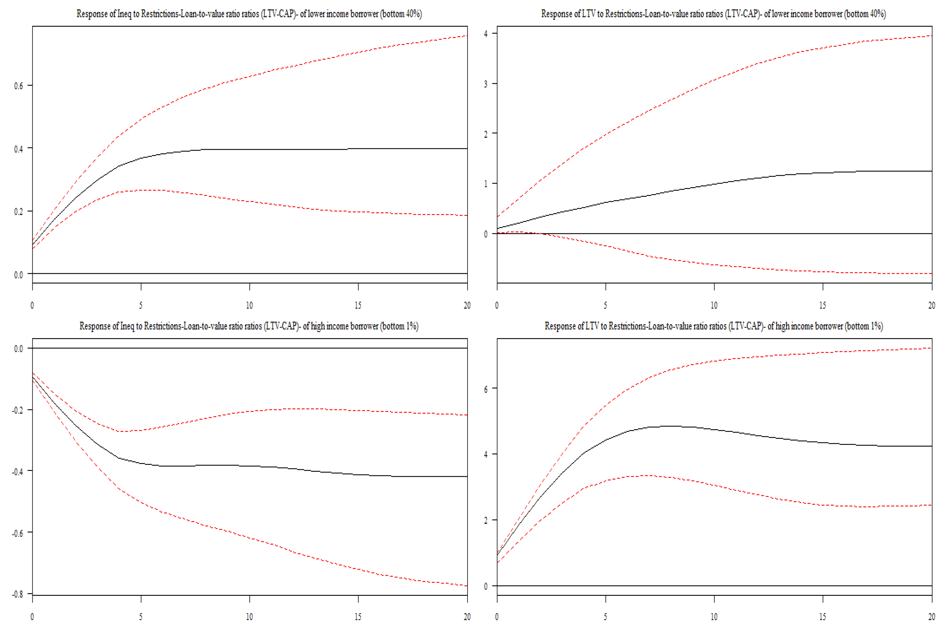
Figure 2 and Column 1 show that when the CB responds to any crises through macroprudential policy instruments using the LTV ratio to lower-income borrowers (the bottom 40% of the income distribution), there is a further increase in income inequality in these countries, following a one percent standard deviation shock to the LTV ratio of lower-income borrowers and attaining a maximum impact of 0.25, five years after the shock stabilized. However, these results are insignificant.
Moreover, in Column 1, a negative and insignificant impact was documented on income inequality following a tightening by the CBs through macroprudential policy instruments in response to crises by tightening the LTV ratio of high-income borrowers (the top 1% of the income distribution). The findings show that, following a one percent standard deviation shock to the LTV ratio of high-income borrowers (the top 1% of the income distribution), income inequality responds negatively, reaching a maximum effect of 0.49 after five years.
The logic behind the insignificant impact of restrictive loan-to-value (LTV) ratios on the income of both lower-income and high-income borrowers in emerging markets can be attributed to the broader financial and economic context.
For lower-income borrowers, restrictive LTV ratios often have a minimal effect because access to credit is already constrained by limited income, high interest rates, and inadequate financial infrastructure, meaning that even restrictive LTV ratios do not significantly change their borrowing capacity or income. For high-income borrowers, the impact is also negligible as they typically have alternative financial resources and investment opportunities that are less affected by LTV restrictions. Moreover, in emerging markets, where financial markets might be less developed or less efficient, high-income individuals often have greater access to informal lending channels or international financial resources, diminishing the influence of local LTV regulations. Thus, in both cases, the restrictive LTV ratios are less impactful due to the pre-existing financial constraints for lower-income borrowers and the broader range of financial options available to high-income borrowers. These findings are in line with the results documented by Tzur-Ilan (2016), Acharya et al. (2017), Frost and van Stralen (2017) and Carpantier et al. (2018).
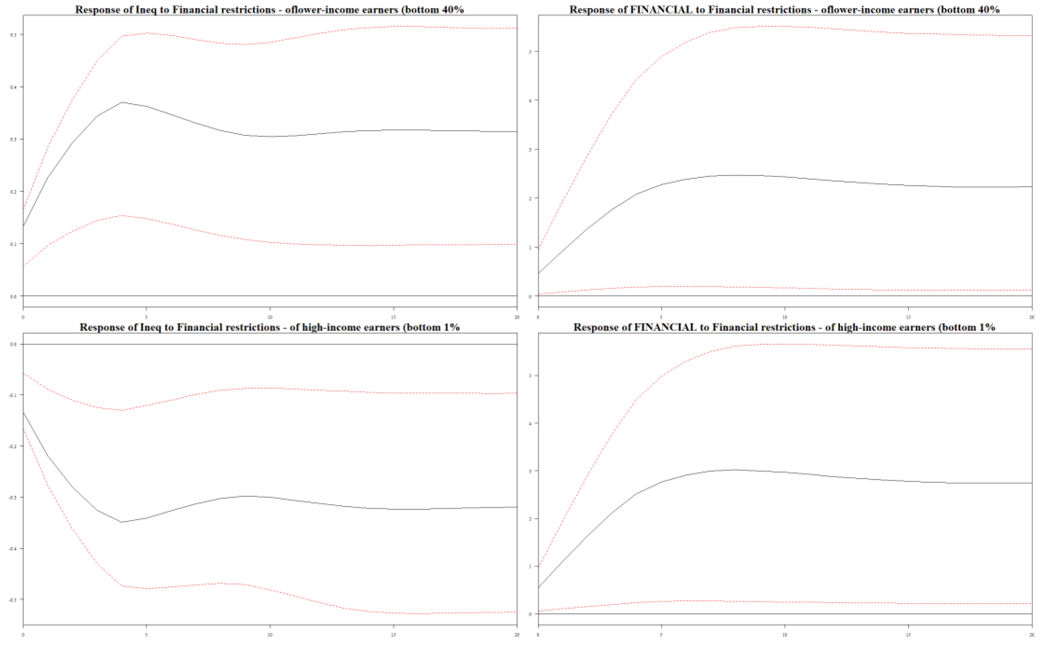
Column 1 of Figure 3 shows that a tightening in macroprudential policy instruments through financial restrictions (FNCE) on lower-income households (the bottom 40% of the income distribution) leads to a positive response in income inequality. Following a one percent standard deviation shock to the financial restrictions on lower-income borrowers (the bottom 40% of the income distribution) and attaining a maximum impact of 0.39 five years after the shock, the economy stabilizes. The results further show that the impact is persistent over time. In Column 2, as a result of the restrictions on the financial access of the top 1% of the income distribution, income inequality responds negatively, reaching a maximum effect of 0.34 after five years and stabilizing.
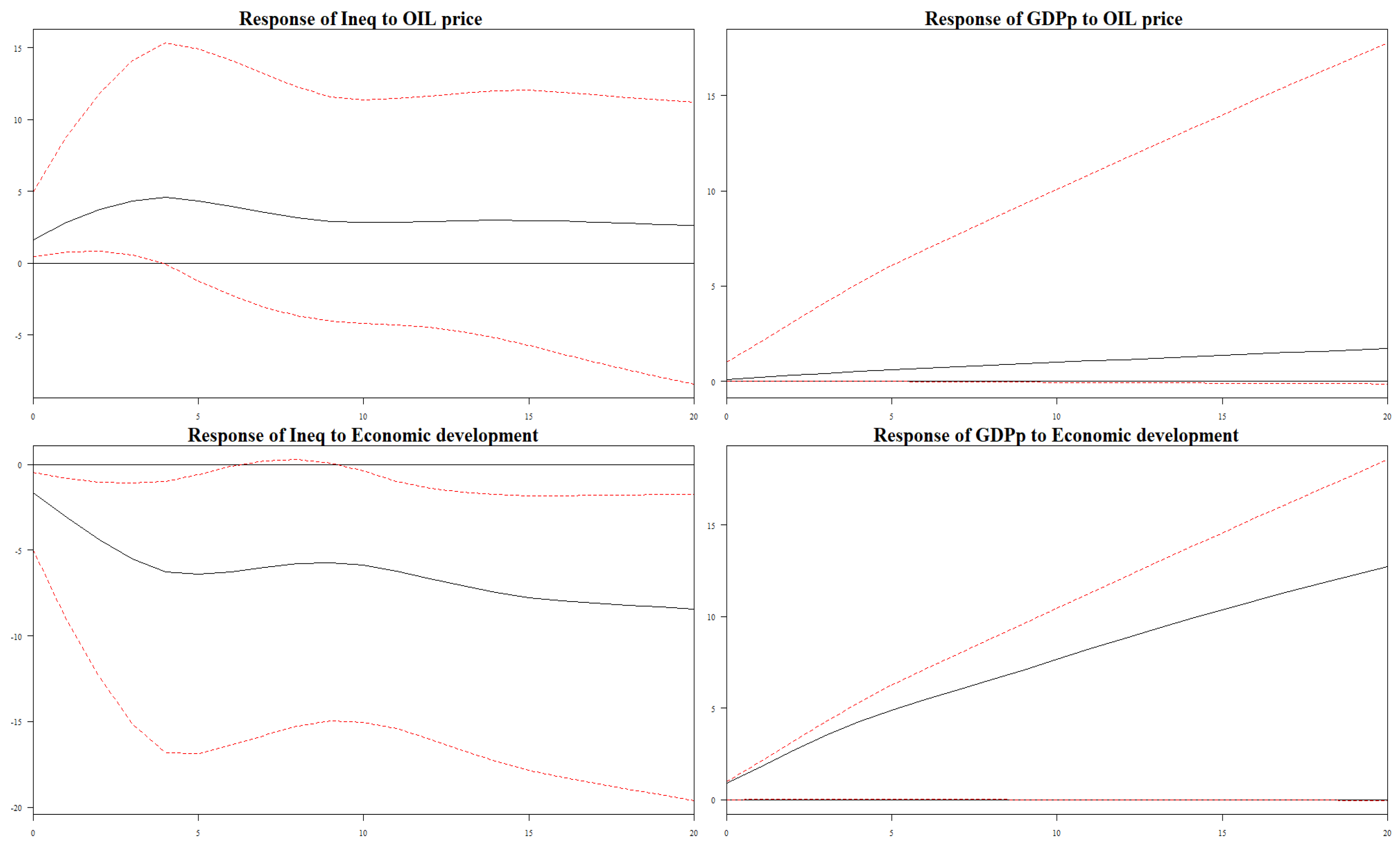
The study then controlled for the oil price shock, economic development, monetary policy through money supply, and fiscal policy through government spending, which were found in the literature to further explain the impact of macroprudential policy on income inequality. Figure 4, in Column 1, presents the findings of the impact of oil price and economic development (GDPp) income inequality. The findings show that, following a one percent standard deviation shock on the oil price (OIL price), income inequality responds positively, reaching a maximum effect of 0.4 after six years. Oil prices significantly impact income inequality in countries reliant on oil exports.
Therefore, the results indicate that high dependence can lead to income disparities as revenues from oil exports are directed towards elites or specific industries, leaving other sectors and individuals with limited economic benefits. Employment opportunities also vary, with rising oil prices boosting job opportunities and income for workers in the oil sector. However, this may not benefit the wider population, as these jobs are specific to the oil industry and may not create sufficient employment opportunities in other sectors. Conversely, low oil prices can lead to job losses and reduced income levels, further exacerbating income inequality. Government revenue and social programs also play a role in income inequality. High oil prices can hinder efforts to diversify the economy, as countries may become overly reliant on oil revenues, limiting opportunities for income growth across different sectors and contributing to long-term income inequality. Conversely, lower oil prices may incentivize governments to diversify their economies, promoting the growth of non-oil industries and potentially reducing income inequality. When economic development and economic growth were controlled, it was found that income inequality responded negatively.
Economic growth is an increase in the capacity of an economy to produce goods and services compared from one period to another. While economic development is a set of programs, policies, or activities that seek to improve the economic well-being and quality of life of a community, these variables are so significant when investigating the impact of macroprudential policies on income inequality.
The results documented in Figure 4, in Column 2, show that following a one percent standard deviation shock to economic development and economic growth, income inequality responds negatively, reaching a maximum effect of 0.07 after five years. The logic behind the negative impact of economic development on income inequality is that it is due to various factors such as job expansion, increased labor productivity, and investments in education and health care.
These factors contribute to a reduction in income inequality as lower-income individuals gain access to better-paying jobs and improve their living standards. Economic growth also generates tax revenues for social welfare programs, redistribution measures, and infrastructure investments, further alleviating income inequality. Ultimately, economic development positively impacts income distribution by creating a conducive environment for economic opportunities and social policies that foster equal income distribution.
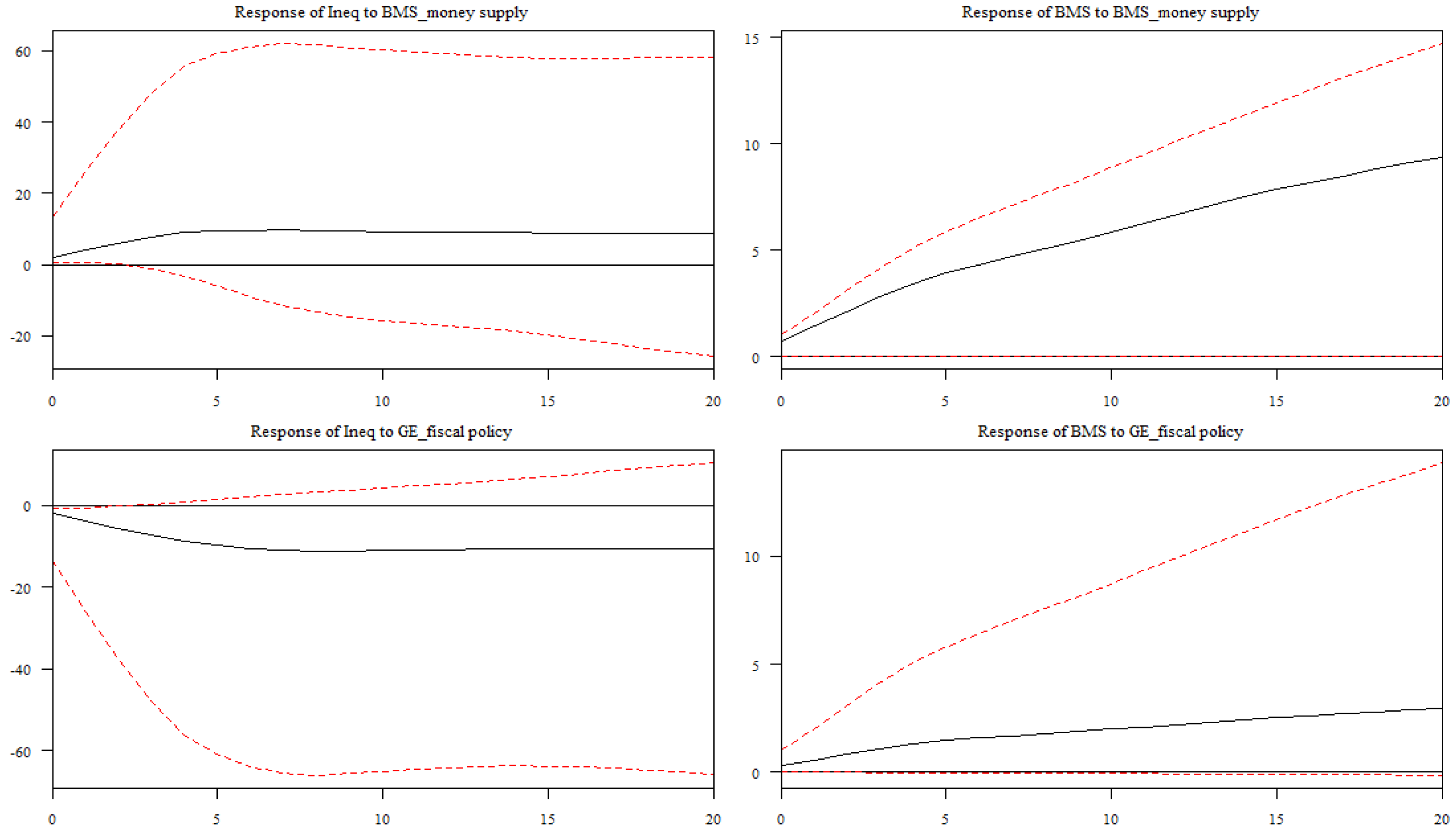
Lastly, Figure 5 in Column 1 contains the impulse response of income inequality following the shock on monetary policy and a fiscal policy. The finding reveals that, following a one percent standard deviation shock on the money supply (BMS), income inequality responds positively, reaching a maximum effect of 0.1 after five years. The finding signifies that the money supply significantly contributes to income inequality in these countries. Monetary policy can contribute to income inequality through various mechanisms. Lowering interest rates stimulates borrowing and spending, boosting the economy and job creation. However, this benefits wealthier individuals with access to credit and investments, widening the wealth gap.
During economic downturns, central banks often inject money into the economy, benefiting asset holders and exacerbating income inequality. Low interest rates may also lead to higher asset prices, benefiting the wealthy and leaving the less affluent struggling to keep up with rising costs.
Figure 5 in, Column 2, On the other hand, income inequality responds negatively following a one percent standard deviation shock on government spending, reaching a maximum effect of 0.18 after six years and then converging to the steady-state region. Government expenditures can reduce income inequality by implementing measures that redistribute wealth and provide resources to the less privileged. Social welfare programs, progressive taxation schemes, and investments in education and infrastructure can improve living standards for low-income individuals, narrowing the gap between the rich and the poor. These measures also create opportunities for upward mobility and enhance the income-earning potential of disadvantaged groups, ultimately contributing to a more equitable society.

4.1.1. Discussion of the BPVAR Results

In emerging markets, stringent debt-to-income (DTI) and financial ratios can exacerbate income inequality among lower-income borrowers due to their restrictive nature. These strict ratios limit the borrowing capacity of individuals with lower incomes, making it challenging for them to access necessary credit for investment, homeownership, or entrepreneurial activities. As a result, lower-income borrowers may be unable to take advantage of opportunities that could enhance their economic status, while higher-income individuals, who have more financial flexibility, can more easily meet these requirements and secure loans. This disparity in access to credit can widen the gap between the wealthy and the less affluent, as the latter group is disproportionately affected by the stringent requirements, which stifle their ability to improve their financial situation and reduce income inequality.
While for the high-income borrowers, stringent debt-to-income (DTI) and financial ratios can paradoxically help reduce income inequality among high-income borrowers by promoting more prudent lending practices and ensuring fairer financial conditions. For high-income individuals, these strict ratios often serve as a regulatory tool to prevent excessive borrowing and over-leverage, which can lead to financial instability. By enforcing these ratios, lenders ensure that even high-income borrowers are not accumulating unsustainable levels of debt, thereby encouraging responsible financial behavior. This approach helps stabilize the financial system and prevents speculative excesses that could disproportionately benefit the wealthy, thus fostering a more balanced distribution of credit and resources. Moreover, by maintaining financial discipline across all income levels, including the affluent, these ratios contribute to a healthier and more equitable economic environment, indirectly benefiting lower-income groups by creating a more stable and inclusive financial market.
Strict loan-to-value (LTV) ratios in emerging markets do not significantly impact income inequality, as lower-income borrowers are less affected by these regulations. High-income borrowers, with their financial stability and alternative funding sources, can easily meet LTV requirements, thereby ignoring the underlying structural inequalities in credit access and wealth distribution (Zungu & Greyling, 2023)
Oil prices in emerging markets can worsen income inequality by disproportionately affecting lower-income households, who spend more on energy. High-income individuals or those in the oil sector may benefit from rising oil prices through increased investment returns or energy revenues. This leads to higher living expenses for the less affluent, while the wealthy may see financial gains or have greater means to absorb such costs. Government spending on education, healthcare, and social welfare programs can help reduce income inequality in emerging markets by improving access to essential services and creating opportunities for disadvantaged populations. Economic development often leads to growth in sectors providing better job opportunities and higher wages, uplifting lower-income groups. Investments in infrastructure and public services can enhance economic mobility and support small businesses, further reducing disparities. Targeting resources towards poverty alleviation and income redistribution directly addresses structural inequalities, promoting more equitable economic growth and reducing income inequality.
Lastly, the rise in money supply in emerging markets can worsen income inequality by causing inflation, disproportionately impacting lower-income households. Wealthier individuals may benefit from asset price increases and inflation hedges, widening the income gap.

4.2. Empirical Results of the Robustness and Sensitivity Analysis Using the BGMM

For robustness and sensitivity analysis, the Bayesian GMM, FE, and FMOLS techniques were developed to investigate the current subject matter in emerging markets. The main aim of using the Bayesian GMM, FE, and FMOLS was to generate the coefficient or elasticity values rather than just showing the impulse response.
The use of benchmark models has become the most appealing practice in modern econometric modelling to verify the robustness of the empirical findings. We believe that the study would yield more grounded results if another model was used that would communicate the results in a coefficient context but further account for endogeneity in the model and further cooperate with the Bayesian econometrics as it had been done in the main model (PBVAR). The results of the BGMM are presented in Table 4, and these results complement the IRF of the PBVAR. The results drawn from the BGMM further signify the positive impact of macroprudential policy instruments on income inequality, as can be seen from the models under SWIID, incPalma-ratio, and incPT10, where in all these models, macroprudential instruments adopted in this study contain a positive sign, while for incPT1, the results had a negative sign.
The findings that reveal that, regardless of the variable used to quantify income inequality, the effect of macroprudential policy instruments on income inequality yields similar results in this region and model the PBVAR, BGMM, FE, and FMOLS models reported in Appendix A Table A1 and Table A2 provide robust evidence of a significant contributional impact of macroprudential policy on income inequality, however with an insignificant impact on loan-to-value ratio (LTV).

5. Conclusion and Policy Recommendations

The current study aims to contribute to the literature by investigating the impact of macroprudential policy measures on income inequality from a different angle than what has been done in the literature. This study focuses on emerging economies using BPVAR and the BGMM. The study also used single equation methods such as the FE and FMOLS to further verify that the results of the baseline model are not sensitive to the variables adopted by including inflation in the model. To the best of the author’s knowledge, no studies have, yet investigated the impact of macroprudential instruments (DTI ratio, LTV ratio, and financial restrictions) on income inequality, if the impact of the restrictions of these instruments on the income inequality of the lower-income borrowers (bottom 40% of the income distribution) and the high-income borrowers (bottom 1% of the income distribution) is observed. The argument was further extended by including the oil price monetary policy using the money supply, fiscal policy using government expenditure, and economic development in the model in order to further find out how income inequality responds to these variables. Our findings yielded some interesting results, as they show that macroprudential policy instruments, such as sticker LTV, DTI ratios, and financial instruments, exacerbate income inequality for lower-income borrowers (the bottom 40% of the income distribution). While tightening for high-income borrowers (the bottom 1 of the income distribution), these policies reduce income inequality in emerging economies. However, the impact of sticker LTV is insignificant on the emerging markets.
These results demonstrate that the poorer segment bears the impact of the implementation of these types of macroprudential policies, while these policies are helpful for the redistribution of wealth by lowering the income and wealth of the wealthy segment.
On the other side, the oil price is found to promote income inequality, as the results show that income inequality increases adversely in response to an unanticipated 1% increase in the oil price. At the same time, economic development was found to play a crucial role in reducing income inequality in these countries. This is evident from the data, which show that income inequality decreases adversely in response to unanticipated 1% increases in economic development. The findings reveal that tightening of monetary policy, particularly the money supply, contributes to high income inequality, while an improvement in economic development and an increase in government expenditure play a crucial role in reducing income inequality in these countries.
The results emphasise that for policy makers to address income inequality among lower-income borrowers in emerging markets, a novel policy recommendation would be to implement a progressive Debt-to-Income (DTI) Ratio System. This system would involve tailoring DTI ratio thresholds based on income brackets, ensuring that lower-income borrowers have access to credit with more lenient DTI requirements, while higher-income borrowers face stricter limits. By doing so, the policy aims to provide greater access to affordable credit for those who need it most, while also mitigating the risks of over-leverage among wealthier individuals. This progressive approach would help lower-income households by allowing them to take on manageable levels of debt that are proportional to their income, thereby improving their financial stability and reducing income disparities.
In conjunction with the progressive DTI Ratio System, the policy could include targeted financial literacy programs and debt management support for lower-income borrowers. These programs would educate borrowers on responsible credit use and effective debt management strategies, further enhancing their ability to benefit from more accessible credit. By combining relaxed DTI ratios with educational initiatives, the policy would not only facilitate better access to credit but also empower lower-income individuals with the knowledge needed to maintain financial stability, ultimately contributing to a reduction in income inequality and fostering more equitable economic growth in emerging markets.
Moreover, on the oil price and money supply, the proposed plan for policymakers should involve a petroleum-linked basic income program that distributes oil revenue to lower-income households, thereby reducing income inequality. It also includes a Monetary Supply Stabilization Fund to maintain financial stability and prevent excessive inflation, thereby leveraging oil wealth and a controlled money supply for equitable income distribution.

Author Contributions

Conceptualization, L.T.Z., L.G.; methodology, L.T.Z.; software, L.T.Z.; validation, L.T.Z.; formal analysis, L.T.Z.; writing—original draft preparation, L.T.Z.; writing—review and editing, L.T.Z., L.G.; visualization, L.T.Z.; supervision, L.G. All authors have read and agreed to the published version of the manuscript.

Funding

This research was funded by the National Research Foundation (NRF) bursary scheme, Grant number: 140829.

Institutional Review Board Statement

The study was conducted in accordance with the Declaration of University of Zululand, and approved by the Ethics Committee of University of Zululand (protocol code UZREC 171110-030 PGD 2021/62 and date of approval: 8 December 20).

Data Availability Statement

Publicly available datasets were analysed in this study. This data can be found here: World Development Indicators. (WDI)A (2023), World Bank Washington, D.C. Available online: http://data.worldbank.org/data-catalog/world-development-indicators (accessed 24 February 2023), and Solt, F. (2021). Measuring Income Inequality Across Countries and Over Time: The Standardized World Income Inequality Database. Social Science Quarterly, 101:1183–1199. SWIID Version 9.2, December 2021. Available online: https://fsolt.org/swiid/ (accessed on 24 May 2021). Further inquiries can be directed to the corresponding author.

Acknowledgments

I thank everyone who attended the Management of Business and Legal Initiatives (MBALI) (2023) conference in Richards Bay for their invaluable input during the early stages of this research. I also thank the University of Zululand’s Department of Economics staff for their constructive criticism and helpful suggestions for this paper. Finally, I would like to express my gratitude to my language editor, Mrs H. Henneke, hennekeh@wcsisp.co.za, for her valuable and consistent input. Thank you so much!

Conflicts of Interest

The authors declare no conflict of interest. Additionally, the funders had no role in the design of the study; in the collection, analyses, or interpretation of data; in the writing of the manuscript, or in the decision to publish the results.
1.
The DTI ratio of lower-income borrowers (the bottom 40% of the income distribution) and high-income borrowers (the top 1% of the income distribution), as well as the LTV ratio of lower-income borrowers (the bottom 40% of the income distribution) and high-income borrowers (the top 1% of the income distribution).

Appendix A

Figure A1. A: Line and Autocorrelation Diagnostic Plots of the Posterior Estimates.
Preprints 116560 g0a1
Unlike the BGMM model, for the single equation model, the fixed effects, and FMOLS, we focus on three variables to capture income inequality, namely the SWIID, Q401 and Q1. The results of the FF are reported in Table A1. This result complements the IRF of the BPVAR and BGMM.
Table A1. Macroprudential policy and income inequality: FE model.
Variables SWIID incPT10 incPT1
Debt-to-Income ratio (DTI) 2.78**[0.88] 2.30**[0.32] -1.13**[-0.48]
Loan-to-Value ratio (LTV) 2.57[5.00] 1.98[2.00] -2.09**[3.94]
Financial instrument (FNCE) 1.06**[0.06] 1.96**[0.22] -2.00**[1.00]
Government spending (GE) -2.93*** [1.07] -1.99** [0.98] -1.33**[0.31]
Broad money supply (MBS) 1.90**[0.28] 2.90**[1.02] 2.93**[0.28]
Economic development (GDPp) -2.83** [1.00] -2.30**[1.15] -1.90** [0.50]
Oil price (OIL price) 1.80**[0.28] 2.93** [0.32] 2.33[4.28]
Inflation (INFL) 0.06**[0.009] 0.23[1.10] 0.90**[0.10]
***, **, * reflect the 1%, 5%, 10% levels of significance, respectively. Source: Author’s illustration based on data SWIID (Solt 2021; WDI 2023).
Lastly, we then further estimated the FMOLS model considering that main advantages of FMOLS method are that the OLS estimator under this method is corrected for the endogeneity and serial correlation. For the FMOLS was carried out with the non-prewhitened Barlett kernel, Newey-West fixed bandwidth = 40.000 . Table A2 reports the results of the FMOLS outputs.
Table A2. Macroprudential policy and income inequality: FMOLS.
Variables SWIID incPT10 incPT1
Debt-to-Income ratio (DTI) 0.87**[0.20] 2.93***[0.32] -2.04[2.56]
Loan-to-Value ratio (LTV) 1.80[2.48] 2.00[1.98] -1.94[1.70]
Financial instrument (FNCE) 2.60**[1.00] 1.69***[0.22] -1.78**[0.43]
Government spending (GE) -1.03** [0.25] -2.83*** [0.85] -2.87***[0.27]
Broad money supply (MBS) 1.03**[0.32] 1.93**[0.32] 2.44**[0.56]
Economic development (GDPp) -2.30**[0.75] -1.93**[0.55] -1.37**[0.27]
Oil price (OIL price) 2.00**[0.91] 0.43[1.09] 2.34 [3.56]
Inflation (INFL) 0.43***[0.03] 1.10**[0.32] 2.06*** [0.96]
R2 0.9345 0.8857 0.9154
***, **, * reflect the 1%, 5%, 10% levels of significance, respectively. Source: Author’s illustration based on data SWIID (Solt 2021; WDI 2023).
The results further complement the results of the IRF of the BPVAR, BGMM, and FF models. For the FMOLS Diagnostic Test, it shows that the model has adequate supply R 2 of 0.93%, 0.88%, and 91%, respectively), which indicates that the regression model has a robust goodness-of-fit and that the variations in income inequality are fully explained by variations in the DTI, LTV, FNCE, GE, MBS, GDPp, oil price, and INFL.

References

  1. Acharya, V.K,, Crosignani, B.M., Eisert, T., & McCann, F. (2017). The Anatomy of the Transmission of Macroprudential Policies: Evidence from Ireland. Presented at 16th International Conference on Credit Risk Evaluation, Interest Rates, Growth, and Regulation, Ireland. Evidence from Ireland.
  2. Adarov, M.A. Adarov, M.A. & Tchaidze, M.R. (2011). Development of financial markets in Central Europe: The case of the CE4 countries. International Monetary Fund 111, 11–101.
  3. Alvaredo, F., Chancel, L., Piketty, T., Saez, E. & Gabriel, Z. (2018). The elephant curve of global inequality and growth. AEA Papers and Proceedings 108, 103–08. [CrossRef]
  4. Andries, A.M. Andries, A.M. & Melnic, F. (2019). Macroprudential Policies and Economic Growth. Review of Economic and Business Studies 12, 95–112.
  5. Arregui, N., Benes, J., Krznar, I., Mitra, S. & Santos, A.O. (2013). Evaluating the Net Benefits of Macroprudential Policy: A Cookbook. IMF Working Paper No. 13/167, Monetary and Capital Markets, Research. Washington, DC: IMF. Available online: https://www.imf.org/external/pubs/ft/wp/2013/wp13167.pdf (accessed on 20 May 2021).
  6. Atkinson, T. (2014); Public Economics in an Age of Austerity; New York; Routledge. [Google Scholar]
  7. Bernanke, Ben. 2015; Monetary Policy and Inequality. Ben Bernanke’s Blog at Brookings. Washington, DC; White House. [Google Scholar]
  8. Bivens, J. (2015). Gauging the Impact of the Fed on Inequality during the Great Recession. Hutchins Center on fiscal & monetary Policy at Brooking’s, Working Paper No. 12. Available online: https://files.epi.org/2015/quantitative-easing-and-inequality-josh-bivens.pdf (accessed on 2 February 2022).
  9. Borio, C., Furfine, C. & Lowe, P. (2001). Procyclicality of Financial Systems and Financial Stability. BIS Papers. No.1. Basle; Bank for International Settlements.
  10. Canova, F. Canova, F. & Ciccarelli, M. (2004). Forecasting and turning point predictions in a Bayesian panel VAR model. Journal of Econometrics 120, 327–359.
  11. Carpantier, J., Olivera, J. & Van Kerm, P. (2018). Macroprudential policy and household wealth inequality. Journal of International Money and Finance 2018, 85, 262–277. [CrossRef]
  12. Carpantier, J.F., Olivera, J., & van Kerm, P. (2018). Macroprudential policy and household wealth inequality. Journal of International Money and Finance 85, 262–277.
  13. Casiraghi, M., Gaiotti, E. Rodano, L & Secchi, A. (2018). A ‘reverse Robin Hood’? The distributional implications of non-standard monetary policy for Italian households. Journal of International Money and Finance 2018, 85, 215–35.
  14. Cerutti, E., Claessens, S. & Laeven, L. (2017). The use and effectiveness of macroprudential policies: New evidence. Journal of Financial Stability 28, 203–24. [CrossRef]
  15. Cerutti, E.R., Claessens, S. & Laeven, L. (2016). The use and effectiveness of macroprudential policies: New evidence. Journal of Financial Stability 28, 203–24.
  16. Ciccarelli, M. & Rebucci, A. (2003). Measuring Contagion with a Bayesian Time-Varying coefficient model (September). IMF Working Paper, No. 03/171. Available at SSRN: https://ssrn.com/abstract=880216.
  17. Clerca, L. Clerca, L., Dervizb, A., Mendicinoc, C., Moyend, S., Nikolove, K., Straccaf, L., Suarezg., J. & Vardoulakish, A.P. (2015). Capital regulation in a macroeconomic model with three layers of default. International Journal of Central Banking 11, 9–63.
  18. Crespo-Cuaresma, J. Crespo-Cuaresma, J. & Fernandez-Amadorb, O. (2013). Business cycle convergence in EMU: A first look at the second moment. Journal of Macroeconomics 37, 265–284.
  19. Davityan, K. (2018). The distributive effect of monetary policy: The top one percent makes the difference. Economic Modelling 65, 106–118. [CrossRef]
  20. Dieppe, A., Legrand, R. & van Roye, B. (2016). The Bayesian Estimation, Analysis and Regression toolbox (BEAR). Working Paper, No. 1934. European Central Bank.
  21. Doan T., Litterman, R. & Sims, C. (1984). Forecasting and Conditional Projection Using Realistic Prior Distributions. Econometric Reviews 3, 1–100.
  22. Doepke, M. & Schneider, M. (2006). Inflation and the redistribution of nominal wealth. Journal of Political Economy 114, 1069–1097.
  23. Elekdag, S. & Wu, Y. (2011). Rapid credit growth: Boon or boom-bust? Working Paper, No. 11/241, International Monetary Fund.
  24. Frees, E. (1995). Assessing cross-sectional correlation in panel data. Journal of Econometrics 69, 393–414. [CrossRef]
  25. Friedman, M. (1937). The use of ranks to avoid the assumption of normality implicit in the analysis of variance. Journal of the American Statistical Association 32, 675–701. [CrossRef]
  26. Frost, J. & van Stralen, R. (2017). Macroprudential policy and income inequality. Journal of International Money and Finance 85, 278–290. [CrossRef]
  27. Georgescu, O. & Martin, V.D. (2022). Do macroprudential measures increase inequality? Evidence from the euro area household survey, Working Paper Series, No. 2567, ECB, Frankfurt am Main, June.
  28. Guerello, C. (2018). Conventional and unconventional monetary policy vs. household’s income distribution: An empirical analysis for the Euro Area. Journal of International Money and Finance 85, 187–214. [CrossRef]
  29. Harris, R.D.F. & Tzavalis, E. (1999). Inference for unit roots in dynamic panels where the time dimension is fixed. Journal of Econometrics 91, 201–226.
  30. Hauner, T. (2016). Aggregate wealth and its distribution as determinants of financial crises. The Journal of Economic Inequality 18, 319–338. [CrossRef]
  31. Im, K.S.M., Pesaran, H. & Shin.Y. (2003). Testing for unit roots in heterogeneous panels. Journal of Econometrics 115, 53–74. [CrossRef]
  32. International monetary Fund (IMF) (2014). Staff guidance note on macroprudential policy. IMF Policy Paper, December.
  33. Inui., M., Sudou, N. & Yamada, T. (2017). Effects of Monetary Policy Shocks on Inequality in Japan. Bank of Japan Working Paper, No. 17-e-3. Available online: https://ssrn.com/abstract=2982887 (accessed on 3 January 2022).
  34. Juan-Francisco, A., Gómez-Fernández, N. & Claramunt, C.O. (2018). Effects of unconventional monetary policy on income and wealth distribution: Evidence from United States and Eurozone. Panoeconomicus First-Online (00), 7-7. [CrossRef]
  35. Kostantinou, P., Rizos, A and Stratopoulou, A. (2021). Macroprudential policies and income inequality in former transition economies. Economic Change and Restructuring 55, 1005–1062. [CrossRef]
  36. Lenza, M. & Slacalek. J. (2018). How Does Monetary Policy Affect Income and Wealth Inequality? Evidence from Quantitative Easing in the Euro Area. ECB Working Paper Series, No. 2190/October 201. EU publications. [CrossRef]
  37. Love, I. & Zicchino, L. (2006). Financial development and dynamic investment behavior: Evidence from panel vector autoregression. Quarterly Review of Economics and Finance 46, 190–210.
  38. Manuel Rupprecht, M. (2020). Income and wealth of euro area households in times of ultra-loose monetary policy: Stylised facts from new national and financial accounts data. Austrian Economic Association 47, 281–302.
  39. Martynova, N. (2015). Effect of bank capital requirements on economic growth: A survey. De Nederlandsche Bank Working Paper, No. 467.
  40. Mendicino, C., Hoerova, M., Nikolov, K., Schepens, G. & van den Heuvel, S. (2018). Benefits and costs of liquidity regulation. ECB Working Paper, No. 2169. Available online: https://www.ecb.europa.eu/pub/pdf/scpwps/ecb.wp2169.en.pdf (accessed on 21 July 2023).
  41. Mumtaz, H. & Theophilopoulou, A. (2017). The impact of monetary policy on inequality in the UK. An empirical analysis. European Economic Review 98, 410–423. [CrossRef]
  42. Pesaran, M.H. (2004). General diagnostic tests for cross section dependence in panels. IZA Discussion Paper No. 1240. docs.iza.org/dp1240.pdf.
  43. Piketty, T. (2014); Capital in the 21st Century; Cambridge; Harvard University Press.
  44. Punzi, M.T & Rabitsch, K. (2018). Effectiveness of macroprudential policies under borrower heterogeneity. Journal of International Money and Finance 85, 251–261.
  45. Rajan, R. (2010). Fault Lines: How hidden Fractures Still Threaten the world Economy; Princeton; Princeton University Press.
  46. Reinhart, C.M. & Rogoff, K.S. (2009). Growth in a time of debt. American Economic Review 100, 573–578.
  47. Rubio, M. & Carrasco-Gallego, J.A. (2014). Macroprudential and monetary policies: Implications for financial stability and welfare. Journal of Banking & Finance 49, 326–336.
  48. Rubio, M. & Unsal, F.D. (2017). Macroprudential policy, incomplete information and inequality: The case of low-income and developing countries. IMF Working Paper, No. WPIEA2017059/36. Available online: https://www.imf.org/en/Publications/WP/Issues/2017/03/21/Macroprudential-Policy-Incomplete-Information-and-Inequality-The-case-of-Low-Income-and-44752 (accessed on 21 January 2023).
  49. Saiki, A. & Frost, J. (2014). Does unconventional monetary policy affect inequality? Evidence from Japan. Applied Economics 46, 4445–4454. [CrossRef]
  50. Sarfati, H. Sarfati, H. (2016). OECD. In it together: Why less inequality benefits all. Paris, 2015. p. 332 ISBN 978–264-23266-2. International Social Security Review 68, 115–17. [CrossRef]
  51. Sims, C.A. (1980). Macroeconomics and reality. Econometrica 48, 1–48. [CrossRef]
  52. Solt, F. (2020). The Standardized World Income-inequality Database. Social Science Quarterly 90, 231–242. [CrossRef]
  53. Solt, F. (2021). Measuring Income Inequality Across Countries and Over Time: The Standardized World Income Inequality Database. Social Science Quarterly. 101, pp. 1183–1199, SWIID Version 9.2, December 2021. Available online: https://fsolt.org/swiid/ (accessed on 24 May 2021).
  54. Stiglitz. J. (2015). Inequality and Economic Growth. The Political Quarterly 86, 134–155. [CrossRef]
  55. Taghizadeh-Hesary, F., Yoshino, N. & Shimizu, S. (2018). The Impact of Monetary and Tax Policy on Income Inequality in Japan. ADBI Working Paper 837. Tokyo: Asian Development Bank Institute. Available online: https://www.researchgate.net/publication/325967488_The_Impact_of_Monetary_and_Tax_Policy_on_Income_Inequality_in_Japan (accessed on 23 April 2022).
  56. Tenreyro, S and Thwaites, G. (2016). Pushing on a tring: US Monetary Policy Is Less Powerful in Recessions. American Economic Journal: Macroeconomics 8, 43–74.
  57. Tzur-Ilan, N. (2016).The effect of credit constraints on housing choices: The case of LTV limits. Paper presented at Bank of Israel, Hebrew Universit, Research Department Conference, December 2016; Available online: https://www.boi.org.il/he/NewsAndPublications/PressReleases/Documents/%D7%A0%D7%99%D7%A6%D7%9F%20%D7%A6%D7%95%D7%A8%20%D7%90%D7%99%D7%9C%D7%9F.pdf (accessed on 24 May 2021).
  58. World Development Indicators. World Development Indicators. (WDI)A (2023), World Bank Washington, D.C. Available online: http://data.worldbank.org/data-catalog/world-development-indicators (accessed on 24 February 2023).
  59. Zellner, A., & Hong, C. (1989). Forecasting international growth rates using Bayesian shrinkage and other procedures. Journal of Econometrics 40, 183–202. [CrossRef]
  60. Zellner, A., Hong, C, & Min. C. (1991). Forecasting turning points in international output growth rates using Bayesian exponentially weighted autoregression, time-varying parameter, and pooling techniques. Journal of Econometrics 49, 275–304. [CrossRef]
  61. Zinman, J. (2010). Restricting consumer credit access: Household survey evidence on effects around the Oregon rate cap. Journal of Banking and Finance 34, 546–556. [CrossRef]
  62. Zungu, L.T. & Greyling, L. (2023). Investigating the asymmetric effect of income inequality on financial fragility in South Africa and selected emerging markets: A Bayesian approach with hierarchical priors. International Journal of Emerging Markets Vol. ahead-of-print, No. ahead-of-print. [CrossRef]
  63. Zungu, L.T., Greyling, L. & Mbatha, N. (2023). Nonlinear Dynamics of the Development-Inequality Nexus in Emerging Countries: The Case of a Prudential Policy Regime. Economies 10, 120.
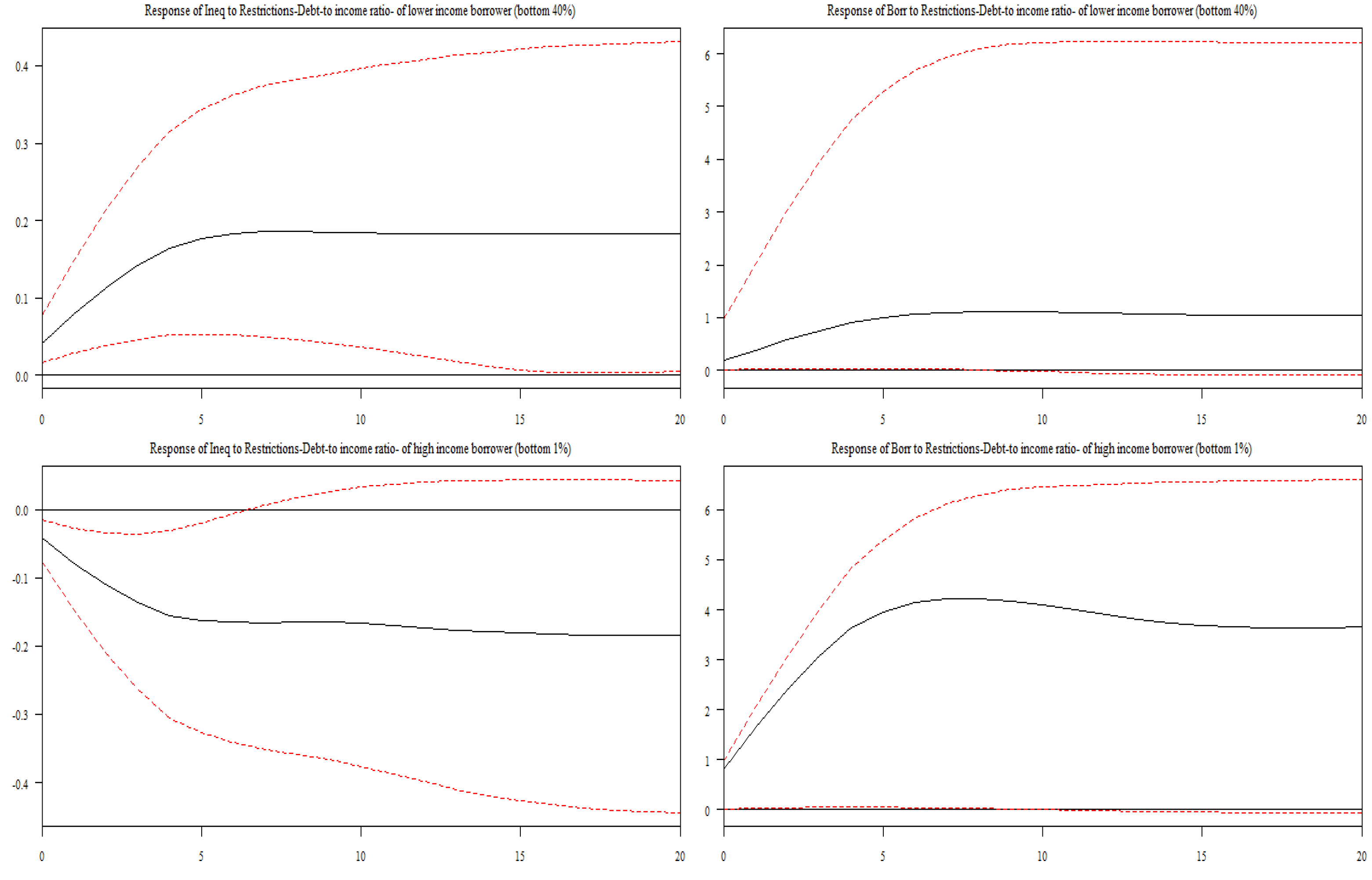
Figure 1. Generated impulse responses of the PBVAR macroprudential policy instruments through the DTI ratio. Note: The black solid lines indicate the posterior median. The red dashed lines indicate the credibility intervals. Source: Author’s illustration based on data SWIID (Solt 2021; WDI 2023).
Preprints 116560 g001
Figure 2. Generated impulse responses of the BPVAR, macroprudential policy instruments through the LTV ratio. Note: The black solid lines indicate the posterior median. The red dashed lines indicate the credibility intervals. Source: Author’s illustration based on data SWIID (Solt 2021; WDI 2023).
Preprints 116560 g002
Figure 3. Generated impulse responses of the BPVAR, macroprudential policy restrictions through the financial instrument. Note: The black solid lines indicate the posterior median. The red dashed lines indicate credibility intervals. Source: Author’s illustration based on data SWIID (Solt 2021; WDI 2023).
Preprints 116560 g003
Figure 4. Generated impulse responses of the BPVAR global shock-oil price and economic development. Note: The black solid lines indicate the posterior median. The red dashed lines indicate credibility intervals. Source: Author’s illustration based on data SWIID (Solt 2021; WDI 2023).
Preprints 116560 g004
Figure 5. Generated impulse responses of the BPVAR, monetary policy and a fiscal policy, government spending shock. Note: The black solid lines indicate the posterior median. The red dashed lines indicate credibility intervals. Source: Author’s illustration based on data SWIID (Solt 2021; WDI 2023).
Preprints 116560 g005
Table 2. Descriptive Statistics and the Panel Stationarity Test.
Descriptive Statistics Im–Pesaran–Shin Harris–Tzavalis
Variables Mea Sth.d Min Max SKW KUR JB-ST JB-P Level 1st ∆ Inte Level 1st ∆ Inte
SWIID 48.29 6.33 8.100 63.50 -0.30 3.04 11.60 0.00 1.77 -5.99*** I(1) 2.37 -15.83*** I(1)
incPalma-r 40.40 5.09 4.00 56.90 -0.98 2.00 9.40 0.00 2.44 -7.40*** I(1) 0.60 -17.99*** I(1)
incPT10 50.54 0.06 30.58 65.44 -0.03 2.19 8.23 0.01 1.48 -4.96*** I(1) 0.68 -4.41*** I(1)
incPT1 45.39 0.04 8.10 63.50 -0.33 2.16 35.51 0.00 2.46 -6.88*** I(1) 3.89 -15.45*** I(1)
DTI 23.56 0.02 0 1 −0.22 2.73 20.33 0.00 No No No No No No
LTV 35.25 0.49 0 1 −0.30 2.00 16.42 0.00 No No No No No No
FNCE 27.94 0.40 0 1 0.10 2.43 13.54 0.00 No No No No No No
OIL price 4.62 0.27 4.08 6.57 -0.12 1.98 80.85 0.00 -0.44 -3.79** I(1) 0.72 -8.80*** I(1)
GE 8.24 8.34 14.48 3.62 -0.23 3.09 76.09 0.00 -1.20 -8.99*** I(1) 0.11 -17.54*** I(1)
MBS 10.92 112.60 75.66 61.90 -0.11 3.87 70.8 0.08 0.33 -6.11 I(1) 2.41 -14.59*** I(1)
GDPp 10.92 112.60 75.66 61.90 -0.11 3.87 70.8 0.08 0.33 -6.11 I(1) 2.41 -14.59*** I(1)
INFL 6.92 112.60 75.66 61.90 -0.11 3.87 70.8 0.08 0.33 -6.11 I(1) 2.41 -14.59*** I(1)
Note: p < 0.1, ** p < 0.05 & *** p < 0.01, while lev and inter denote level and integration, respectively. Mea—mean, SKW—Skewness, KUR—Kurtosis, JB-ST—Jarque–Bera statistics, and lastly, Jarque–Bera probability is denoted by JB-P. Source: Author’s illustration based on data SWIID (Solt 2021; WDI 2023).
Table 3. Cointegration and Cross-Sectional Independence Tests.
Pedroni Tests for Cointegration Tests for Cross-Sectional Independence
Augmented Dickey–Fuller t 6.34 Pr = 0.01 Friedman’s test 111.00 Pr = 0.00
Modified Phillips–Perron t 4.64 Pr = 0.08 Frees’ test 0.82 Pr = 0.00
Phillips Perron t 6.00 Pr = 0.000 Pesaran’s test 12.65 Pr = 0.00
Source: Author’s illustration based on data SWIID (Solt 2021; WDI 2023).
Table 4. Macroprudential policy and income inequality: BGMM.
Variables SWIID incPalma-ratio incPT10 incPT1
Debt-to-Income ratio (DTI) 2.98**(1.00) 3.87**(1.10) 1.39***(0.10) -3.22**(0.89)
Loan-to-Value ratio (LTV) 3.43(2.20) 1.92**(0.31) 1.90(2.20) -1.98(1.80)
Financial instrument (FNCE) 2.01**(0.90) -1.90**(0.50) 2.70***(0.29) -2.90**(0.50)
Government spending (GE) -4.00**(2.00) -2.10**(0.69) -1.90**(0.90) 1.30**(0.22)
Broad money supply (MBS) 2.11***(0.10) 3.77**(1.00) 1.00**(0.10) 2.50**(0.70)
Economic development (GDPp) -3.00**(1.20) -2.04**(0.70) -2.44** (0.80) -3.32**(1.30)
Oil price (OIL price) 2.20***(0.24) 3.09 **(0.90) 2.10**(0.44) 1.90***(0.20)
Inflation (INFL) 2.98**(1.00) 0.49***(0.04) 2.87**(0.89) 2.32**(1.00)
   AR (1): p-value 0.007 0.004 0.005 0.008
   AR (2): p-value 0.320 0.230 0.580 0.450
***, **, * reflect the 1%, 5%, 10% levels of significance, respectively. Source: Author’s illustration based on data SWIID (Solt 2021; WDI 2023).
Disclaimer/Publisher’s Note: The statements, opinions and data contained in all publications are solely those of the individual author(s) and contributor(s) and not of MDPI and/or the editor(s). MDPI and/or the editor(s) disclaim responsibility for any injury to people or property resulting from any ideas, methods, instructions or products referred to in the content.
Copyright: This open access article is published under a Creative Commons CC BY 4.0 license, which permit the free download, distribution, and reuse, provided that the author and preprint are cited in any reuse.
Prerpints.org logo

Preprints.org is a free preprint server supported by MDPI in Basel, Switzerland.

Subscribe

© 2024 MDPI (Basel, Switzerland) unless otherwise stated