Submitted:
01 September 2024
Posted:
04 September 2024
You are already at the latest version
Abstract
Keywords:
Introduction
-
Similar processes in different animal species exhibit a typical lifetime. The last five years have seen publications on various factors, including Genetic Factors [18], Metabolic Rate and Energy Expenditure [19], Evolutionary Pressures [20,21], Reproductive Strategies [22] and Comparative Biology and Genetic Models [23].In our model, the same type of map characterized by parameters describes various processes. Lifetime is determined by setting the parameter values.
- The transition between life and death. In biology, death is a process through which biological systems transform from one state to another [24? ]. This transition is characterized by critical points at which the systems move from order to disorder, akin to phase changes in physical systems. However, there are several problems with this approach [25]: First, biological systems are inherently complex, which renders the application of the simplified models used in physical systems challenging. Second, the interactions within biological systems are often nonlinear and involve multiple feedback loops. Consequently, the identification of phase transitions becomes a complicated task. The last difficulty offers an advantage to our approach, which already implements non-linearity. In our model, instead of implementing the complicated phase transition scenario, the transition from life to death occurs when the mapping ceases to be mathematically defined, which is prevalent in nonlinear dynamics, such as in a logistic map, inverse sine map, square root map, reciprocal map, and exponential map with logarithm [26,27,28,29,30].
1. Terminology
-
- (a)
- System: A specific part (generally small) of the universe under consideration.
- (b)
- Surroundings (or Environment): All external elements that can interact with the system.
- (c)
- Universe: The total combination of the system and its surroundings.
-
Biology [33]
- (a)
- Animate processes: Processes that emphasize mobility, behavior, and sensory responses.
- (b)
- Living processes: Processes that emphasize fundamental life functions and biochemical activities.
2. Logistic Map
3. Nonlinear Recursive Model
3.1. Regular process-living process
3.2. System with both interactions
-
We hypothesize a gradual increase in R. This adjustment facilitates two primary effects:
- (a)
- The system progresses toward chaotic behavior. Associating this increase in chaos with increasing entropy suggests that the increased R aligns with the second law of thermodynamics.
- (b)
- The influence of the environment is modeled by introducing slight randomness in x and C.
-
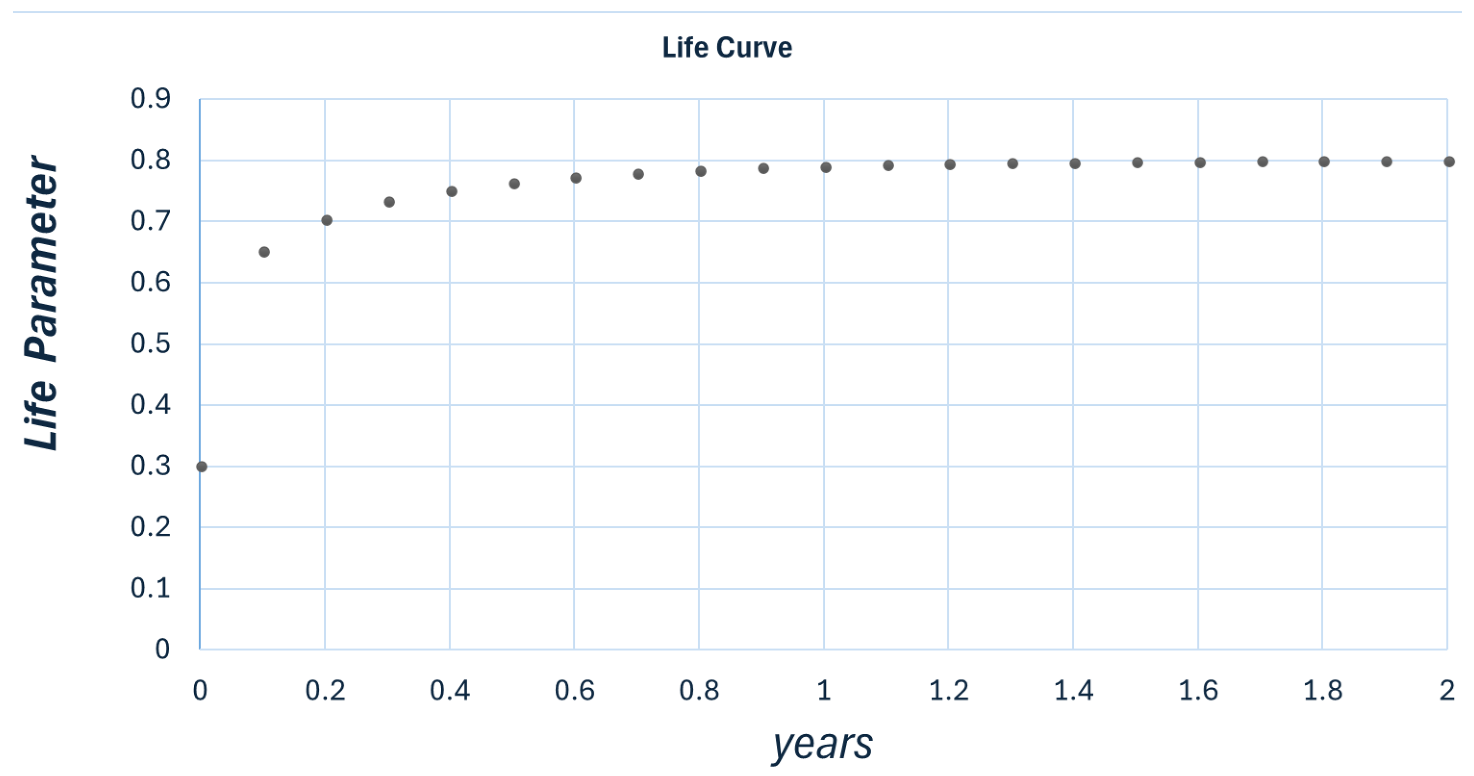
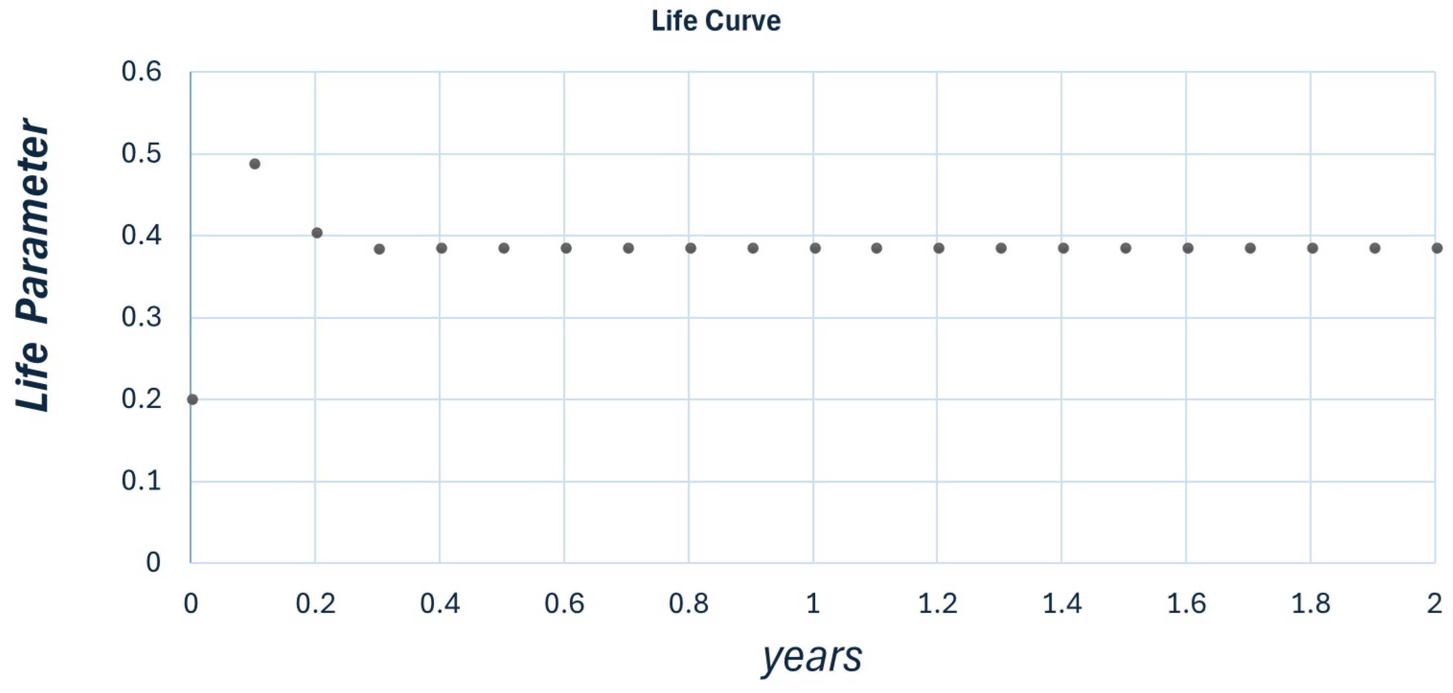
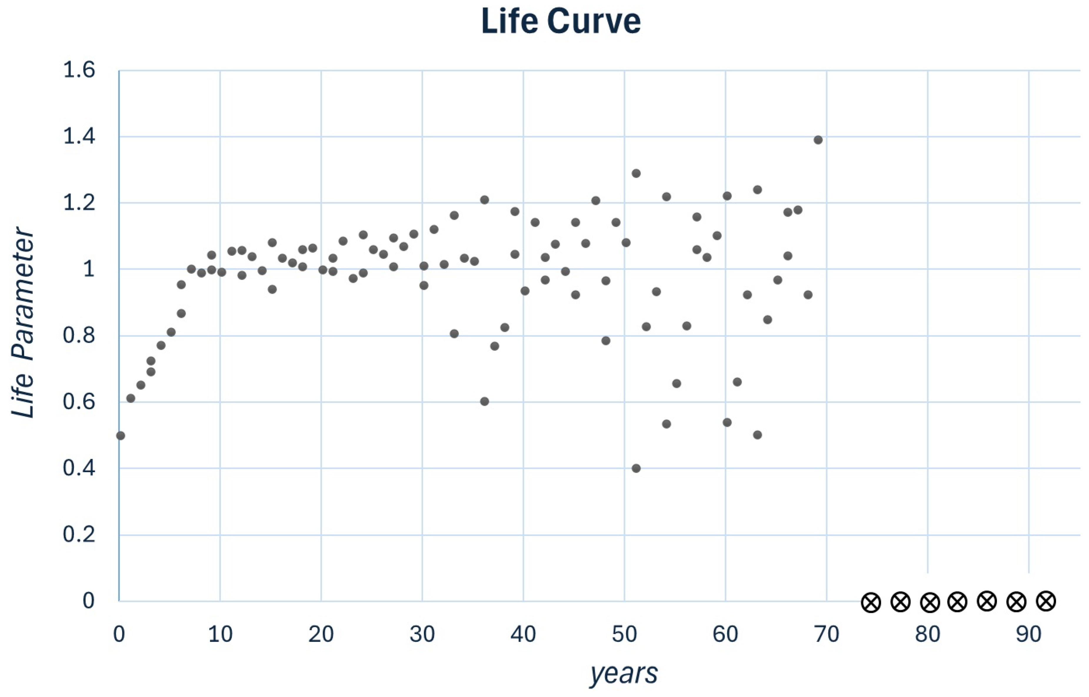
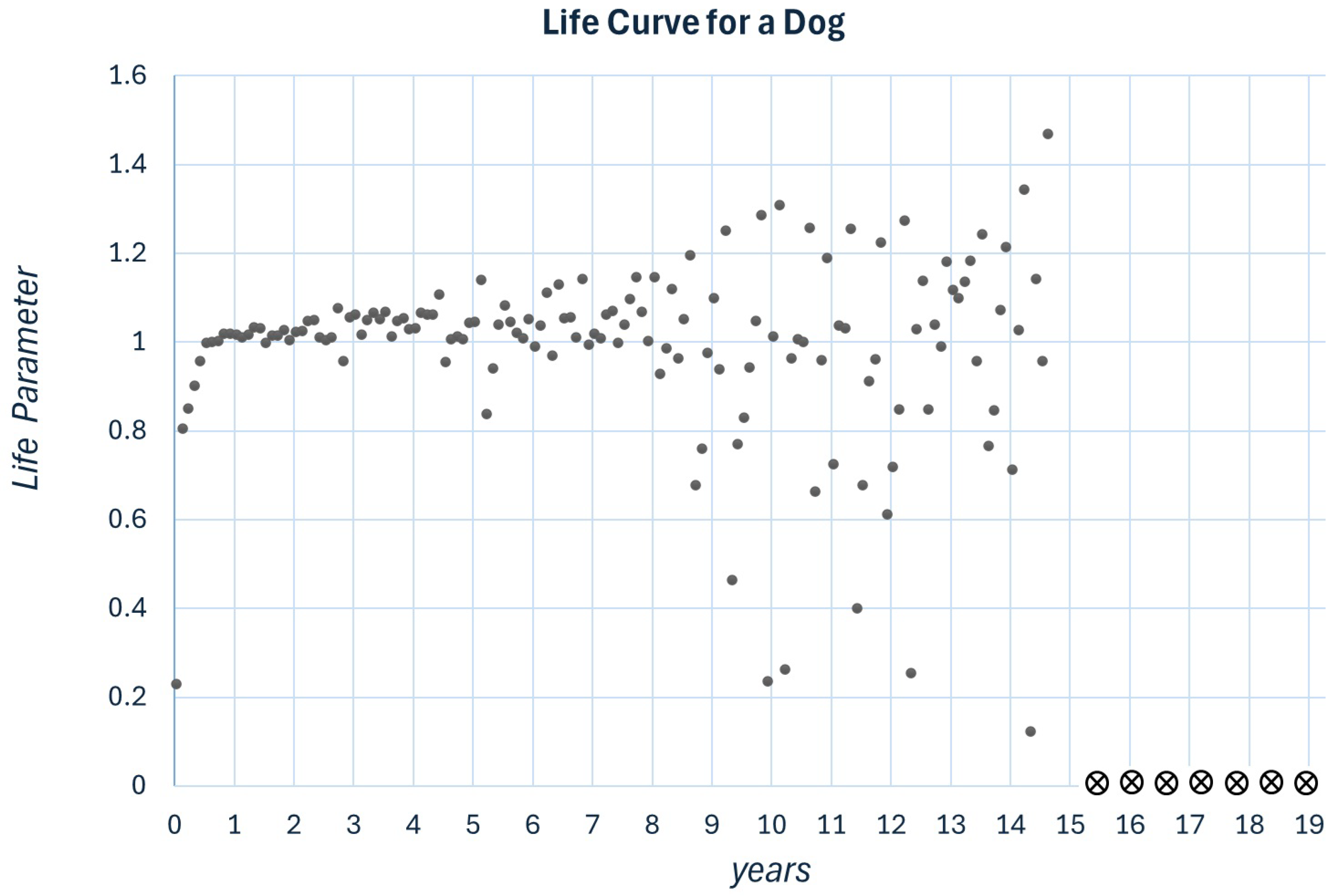
Evolving section:For , x approaches the constant value .
-
Sustainable zone:For x is oscillating randomly around .
-
Aging:For , x represents a process wherein any disorder increases.
-
Death:For the system becomes mathematically undefined. If the progression of x toward a constant value signifies a living process, the absence of a definable evolution of x, whether decreasing, increasing, or stable, indicates that this living process has ceased to exist.
4. Example for Adjusting Parameters to Describe Life Process Type
5. Summary
- Conceptual Understanding: The application of nonlinear dynamics to the study of living processes yields insights that are often not discernible through qualitative analysis alone.
- Simulation: The proposed model facilitates the simulation of unobserved life forms. Although our current study neglects the bifurcation phenomenon common to nonlinear systems, the identification of living processes that exhibit this behavior could significantly contribute to the field and refine our model.
- Theoretical framework. The model provides a robust theoretical framework that assists in hypothesis generation, experimental design, and data interpretation. In our approach, various life processes were classified according to distinct nonlinear mappings. The evolution of a system within a specific category is determined by the numerical values of the mapping parameters. In the case of our mode, this may indicate characteristics such as the lifespan of a process.
References
- Taylor, K. A New Physics Theory of Life. Quanta Magazine 2023.
- Kostic, M.M. Entropy and the Second Law of Thermodynamics: From the microscale to the macroscale (explaining the inefficiency of energy conversion) and the controversial, crucial concept of the arrow of time. Entropy 2020.
- Longdom. Life: A Complex Spontaneous Process Takes Place Against the Background of Nonspontaneous Processes Initiated by the Environment. Journal of Clinical Trials & Research 2020.
- El-Samad, H. Biological feedback control—Respect the loops. Cell Systems 2021, 12, 477–487.
- authors, V. Identification, visualization, statistical analysis and mathematical modeling of high-feedback loops in gene regulatory networks. BMC Bioinformatics 2017, 18, 574. [CrossRef]
- authors, V. Linking fast and slow positive feedback loops creates an optimal bistable switch in cell signaling. Physical Review E 2007, 76, 031924. [CrossRef]
- authors, V. Modulation of dynamic modes by interplay between positive and negative feedback loops in gene regulatory networks. Physical Review E 2018, 97, 042412. [CrossRef]
- Wolf, A. Simplicity and universality in the transition to chaos. Nature 1983, 305, 182–183. [CrossRef]
- Feigenbaum, M. Quantitative universality for a class of non-linear transformations. Journal of Statistical Physics 1978, 19, 25–52. [CrossRef]
- Campbell, N.A.; Reece, J.B.; Urry, L.A.; Cain, M.L.; Wasserman, S.A.; Minorsky, P.V.; Jackson, R.B. Biology; Pearson Education, 2017.
- Clarke, A.; Rothery, P.; Isaac, N.J.B. Thermoregulation in endotherms: evolutionary implications and consequences. Biological Reviews 2016, 91, 97–125.
- Hill, R.W.; Wyse, G.A.; Anderson, M. Animal Physiology; Sinauer Associates, Inc., 2020.
- Moysis, L.; Volos, C.; Jafari, S.; Munoz-Pacheco, J.M.; Kengne, J.; Rajagopal, K.; Stouboulos, I. Modification of the Logistic Map Using Fuzzy Numbers with Application to Pseudorandom Number Generation and Image Encryption. Entropy 2020, 22, 1096. [CrossRef]
- Wang, C.; Ding, Q. A Class of Quadratic Polynomial Chaotic Maps and Their Fixed Points Analysis. Entropy 2019, 21, 658. [CrossRef]
- Song, Y.; Yuan, F.; Li, Y. Coexisting Attractors and Multistability in a Simple Memristive Wien-Bridge Chaotic Circuit. Entropy 2019, 21, 678. [CrossRef]
- Robledo, A. Exploring transitions to chaos in complex systems. Research Outreach 2021. [CrossRef]
- Tolkacheva, E.G.; Grigoriev, R. Nonlinear Dynamics and Chaos in Cardiac Physics. Entropy 2023, 25. [CrossRef]
- Fitzgerald, J.e.a. Genetic determinants of healthy aging and longevity: a systematic review. Current Genetic Medicine Reports 2022, 10, 131–146.
- Grossi, V.; Forte, G.; Sanese, P.; Peserico, A.; Tezil, T.; Lepore Signorile, M. The longevity SNP rs2802292 uncovered: HSF1 activates stress-dependent expression of FOXO3 through an intronic enhancer. Nucleic Acids Research 2018, 46, 5587–600. [CrossRef]
- Atkins, J.; Jylhävä, J.; Pedersen, N.; Magnusson, P.; Lu, Y.; Wang, Y. A genome-wide association study of the frailty index highlights synaptic pathways in aging. medRxiv 2019.
- Willems, S.; Wright, D.; Day, F.; Trajanoska, K.; Joshi, P.; Morris, J. Large-scale GWAS identifies multiple loci for hand grip strength providing biological insights into muscular fitness. Nature Communications 2017, 8, 1–12. [CrossRef]
- Michel, J.P.; Graf, C.; Ecarnot, F. Individual healthy aging indices, measurements and scores. Aging Clinical and Experimental Research 2019, 31, 1719–1725.
- Rose, G.; Sørensen, M.; Dato, S. Genetic determinants of human longevity. MDPI 2019.
- Authors, V. Phase Transitions in Biological Systems with Many Components. ScienceDirect 2023, 100, 032414.
- Herron, L.; Mondal, K.; Schneekloth, J.S.; Tiwary, P. Inferring phase transitions and critical exponents from limited observations with Thermodynamic Maps. arXiv preprint arXiv:2308.14885 2023.
- May, R.M. Simple mathematical models with very complicated dynamics. Nature 1976, 261, 459–467. [CrossRef]
- Devaney, R.L. Transcendental Dynamics and Complex Exponentials. Bulletin of the American Mathematical Society 1978, 84, 1239–1255.
- Feigenbaum, M.J. Quantitative Universality for a Class of Nonlinear Transformations. Journal of Statistical Physics 1978, 19, 25–52. [CrossRef]
- Collet, P.; Eckmann, J.P. Iterated Maps on the Interval as Dynamical Systems. Progress in Physics 1980, 1, 1–248. [CrossRef]
- Guckenheimer, J.; Holmes, P. Structurally Stable Heteroclinic Cycles. Mathematical Proceedings of the Cambridge Philosophical Society 1979, 103, 189–192. [CrossRef]
- Callen, H.B. Thermodynamics and an Introduction to Thermostatistics; Wiley: New York, 1985.
- Atkins, P.; de Paula, J. Physical Chemistry; Oxford University Press: Oxford, 2010.
- Academic, O. Chapter on Animate and Inanimate Matter. Oxford Academic 2020.
- for Majors I, B. The Second Law of Thermodynamics. Lumen Learning 2023.
- MDPI. Life’s Mechanism. MDPI 2023.
- Strogatz, S.H. Nonlinear Dynamics and Chaos: With Applications to Physics, Biology, Chemistry, and Engineering; Westview Press: Boulder, CO, 1994.
- Hilborn, R.C. Chaos and Nonlinear Dynamics: An Introduction for Scientists and Engineers; Oxford University Press: Oxford, UK, 2020.
- Isaacson, E.; Keller, H.B. Analysis of Numerical Methods; Dover Publications: New York, 1994.
- Murray, J.D. Mathematical Biology: I. An Introduction; Springer: New York, 2002.
- Oppenheim, A.V.; Schafer, R.W. Discrete-Time Signal Processing; Pearson: Upper Saddle River, NJ, 2009.


Disclaimer/Publisher’s Note: The statements, opinions and data contained in all publications are solely those of the individual author(s) and contributor(s) and not of MDPI and/or the editor(s). MDPI and/or the editor(s) disclaim responsibility for any injury to people or property resulting from any ideas, methods, instructions or products referred to in the content. |
© 2024 by the authors. Licensee MDPI, Basel, Switzerland. This article is an open access article distributed under the terms and conditions of the Creative Commons Attribution (CC BY) license (http://creativecommons.org/licenses/by/4.0/).


